arXiv:hep-ex/0010031v1 13 Oct 2000
CERN-EP/2000-125 September 19, 2000
Investigation of the Decay of Orbitally-Excited B Mesons and First Measurement of the
Branching Ratio BR( B
∗J→ B
∗π(X ))
The OPAL Collaboration
Abstract
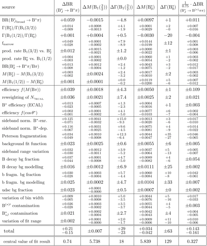
From about 4 million hadronic Z0 decays recorded by the OPAL detector on and near to the Z0 resonance, we select a sample of more than 570 000 inclusively reconstructed B mesons. Orbitally-excited mesons B∗J are reconstructed using Bπ± combinations. In- dependently, B∗ mesons are reconstructed using the decay B∗→Bγ. The selected B∗ candidates are used to obtain samples enriched or depleted in the decay B∗J →B∗π±(X), where (X) refers to decay modes with or without additional accompanying decay parti- cles. From the number of signal candidates in the Bπ± mass spectra of these two samples, we perform the first measurement of the branching ratio of orbitally-excited B mesons decaying into B∗π(X):
BR( B∗J →B∗π(X)) = 0.85+0.26−0.27±0.12,
where the first error is statistical and the second systematic. If B∗J decay modes other than single pion transitions can be neglected the measured ratio corresponds to the branching ratio BR( B∗J →B∗π).
In the framework of Heavy Quark Symmetry, a simultaneous fit to the Bπ± mass spectra of the samples enriched or depleted in B∗J →B∗π±(X) decays yields the mass and the width of the B1(3/2) state, as well as the branching ratio of B∗J mesons decaying into B∗π:
M(B1(3/2)) = ( 5.738+ 0.005−0.006±0.007 ) GeV/c2 Γ(B1(3/2)) = ( 18+ 15 + 29−13−23) MeV/c2
BR( B∗J →B∗π) = 0.74+ 0.12 + 0.21
−0.10−0.15,
where the uncertainties are statistical and systematic, respectively.
(Submitted to Eur. Phys. J.)
The OPAL Collaboration
G. Abbiendi2, K. Ackerstaff8, C. Ainsley5, P.F. ˚Akesson3, G. Alexander22, J. Allison16, K.J. Anderson9, S. Arcelli17, S. Asai23, S.F. Ashby1, D. Axen27, G. Azuelos18,a, I. Bailey26, A.H. Ball8, E. Barberio8, R.J. Barlow16, S. Baumann3, T. Behnke25, K.W. Bell20, G. Bella22,
A. Bellerive9, G. Benelli2, S. Bentvelsen8, S. Bethke32, O. Biebel32, I.J. Bloodworth1, O. Boeriu10, P. Bock11, J. B¨ohme14,h, D. Bonacorsi2, M. Boutemeur31, S. Braibant8, P. Bright-Thomas1, L. Brigliadori2, R.M. Brown20, H.J. Burckhart8, J. Cammin3, P. Capiluppi2,
R.K. Carnegie6, A.A. Carter13, J.R. Carter5, C.Y. Chang17, D.G. Charlton1,b, P.E.L. Clarke15, E. Clay15, I. Cohen22, O.C. Cooke8, J. Couchman15, C. Couyoumtzelis13, R.L. Coxe9, A. Csilling15,j, M. Cuffiani2, S. Dado21, G.M. Dallavalle2, S. Dallison16, A. de Roeck8, E. de
Wolf8, P. Dervan15, K. Desch25, B. Dienes30,h, M.S. Dixit7, M. Donkers6, J. Dubbert31, E. Duchovni24, G. Duckeck31, I.P. Duerdoth16, P.G. Estabrooks6, E. Etzion22, F. Fabbri2,
M. Fanti2, L. Feld10, P. Ferrari12, F. Fiedler8, I. Fleck10, M. Ford5, A. Frey8, A. F¨urtjes8, D.I. Futyan16, P. Gagnon12, J.W. Gary4, G. Gaycken25, C. Geich-Gimbel3, G. Giacomelli2,
P. Giacomelli8, D. Glenzinski9, J. Goldberg21, C. Grandi2, K. Graham26, E. Gross24, J. Grunhaus22, M. Gruw´e25, P.O. G¨unther3, C. Hajdu29, G.G. Hanson12, M. Hansroul8,
M. Hapke13, K. Harder25, A. Harel21, M. Harin-Dirac4, A. Hauke3, M. Hauschild8, C.M. Hawkes1, R. Hawkings8, R.J. Hemingway6, C. Hensel25, G. Herten10, R.D. Heuer25,
J.C. Hill5, A. Hocker9, K. Hoffman8, R.J. Homer1, A.K. Honma8, D. Horv´ath29,c, K.R. Hossain28, R. Howard27, P. H¨untemeyer25, P. Igo-Kemenes11, K. Ishii23, F.R. Jacob20,
A. Jawahery17, H. Jeremie18, C.R. Jones5, P. Jovanovic1, T.R. Junk6, N. Kanaya23, J. Kanzaki23, G. Karapetian18, D. Karlen6, V. Kartvelishvili16, K. Kawagoe23, T. Kawamoto23, R.K. Keeler26, R.G. Kellogg17, B.W. Kennedy20, D.H. Kim19, K. Klein11, A. Klier24, S. Kluth32,
T. Kobayashi23, M. Kobel3, T.P. Kokott3, S. Komamiya23, R.V. Kowalewski26, T. Kress4, P. Krieger6, J. von Krogh11, T. Kuhl3, M. Kupper24, P. Kyberd13, G.D. Lafferty16, H. Landsman21, D. Lanske14, I. Lawson26, J.G. Layter4, A. Leins31, D. Lellouch24, J. Letts12, L. Levinson24, R. Liebisch11, J. Lillich10, B. List8, C. Littlewood5, A.W. Lloyd1, S.L. Lloyd13,
F.K. Loebinger16, G.D. Long26, M.J. Losty7, J. Lu27, J. Ludwig10, A. Macchiolo18, A. Macpherson28,m, W. Mader3, S. Marcellini2, T.E. Marchant16, A.J. Martin13, J.P. Martin18,
G. Martinez17, T. Mashimo23, P. M¨attig24, W.J. McDonald28, J. McKenna27, T.J. McMahon1, R.A. McPherson26, F. Meijers8, P. Mendez-Lorenzo31, W. Menges25, F.S. Merritt9, H. Mes7, A. Michelini2, S. Mihara23, G. Mikenberg24, D.J. Miller15, W. Mohr10, A. Montanari2, T. Mori23, K. Nagai8, I. Nakamura23, H.A. Neal12,f, R. Nisius8, S.W. O’Neale1, F.G. Oakham7, F. Odorici2,
H.O. Ogren12, A. Oh8, A. Okpara11, M.J. Oreglia9, S. Orito23, G. P´asztor8,j, J.R. Pater16, G.N. Patrick20, J. Patt10, P. Pfeifenschneider14,i, J.E. Pilcher9, J. Pinfold28, D.E. Plane8, B. Poli2, J. Polok8, O. Pooth8, M. Przybycie´n8,d, A. Quadt8, C. Rembser8, P. Renkel24, H. Rick4,
N. Rodning28, J.M. Roney26, S. Rosati3, K. Roscoe16, A.M. Rossi2, Y. Rozen21, K. Runge10, O. Runolfsson8, D.R. Rust12, K. Sachs6, T. Saeki23, O. Sahr31, E.K.G. Sarkisyan22, C. Sbarra26,
A.D. Schaile31, O. Schaile31, P. Scharff-Hansen8, M. Schr¨oder8, M. Schumacher25, C. Schwick8, W.G. Scott20, R. Seuster14,h, T.G. Shears8,k, B.C. Shen4, C.H. Shepherd-Themistocleous5,
P. Sherwood15, G.P. Siroli2, A. Skuja17, A.M. Smith8, G.A. Snow17, R. Sobie26, S. S¨oldner-Rembold10,e, S. Spagnolo20, M. Sproston20, A. Stahl3, K. Stephens16, K. Stoll10, D. Strom19, R. Str¨ohmer31, L. Stumpf26, B. Surrow8, S.D. Talbot1, S. Tarem21, R.J. Taylor15,
R. Teuscher9, M. Thiergen10, J. Thomas15, M.A. Thomson8, E. Torrence9, S. Towers6, D. Toya23, T. Trefzger31, I. Trigger8, Z. Tr´ocs´anyi30,g, E. Tsur22, M.F. Turner-Watson1,
I. Ueda23, B. Vachon26, P. Vannerem10, M. Verzocchi8, H. Voss8, J. Vossebeld8, D. Waller6, C.P. Ward5, D.R. Ward5, P.M. Watkins1, A.T. Watson1, N.K. Watson1, P.S. Wells8, T. Wengler8, N. Wermes3, D. Wetterling11 J.S. White6, G.W. Wilson16, J.A. Wilson1,
T.R. Wyatt16, S. Yamashita23, V. Zacek18, D. Zer-Zion8,l
1School of Physics and Astronomy, University of Birmingham, Birmingham B15 2TT, UK
2Dipartimento di Fisica dell’ Universit`a di Bologna and INFN, I-40126 Bologna, Italy
3Physikalisches Institut, Universit¨at Bonn, D-53115 Bonn, Germany
4Department of Physics, University of California, Riverside CA 92521, USA
5Cavendish Laboratory, Cambridge CB3 0HE, UK
6Ottawa-Carleton Institute for Physics, Department of Physics, Carleton University, Ottawa, Ontario K1S 5B6, Canada
7Centre for Research in Particle Physics, Carleton University, Ottawa, Ontario K1S 5B6, Canada
8CERN, European Organisation for Nuclear Research, CH-1211 Geneva 23, Switzerland
9Enrico Fermi Institute and Department of Physics, University of Chicago, Chicago IL 60637, USA
10Fakult¨at f¨ur Physik, Albert Ludwigs Universit¨at, D-79104 Freiburg, Germany
11Physikalisches Institut, Universit¨at Heidelberg, D-69120 Heidelberg, Germany
12Indiana University, Department of Physics, Swain Hall West 117, Bloomington IN 47405, USA
13Queen Mary and Westfield College, University of London, London E1 4NS, UK
14Technische Hochschule Aachen, III Physikalisches Institut, Sommerfeldstrasse 26-28, D-52056 Aachen, Germany
15University College London, London WC1E 6BT, UK
16Department of Physics, Schuster Laboratory, The University, Manchester M13 9PL, UK
17Department of Physics, University of Maryland, College Park, MD 20742, USA
18Laboratoire de Physique Nucl´eaire, Universit´e de Montr´eal, Montr´eal, Quebec H3C 3J7, Canada
19University of Oregon, Department of Physics, Eugene OR 97403, USA
20CLRC Rutherford Appleton Laboratory, Chilton, Didcot, Oxfordshire OX11 0QX, UK
21Department of Physics, Technion-Israel Institute of Technology, Haifa 32000, Israel
22Department of Physics and Astronomy, Tel Aviv University, Tel Aviv 69978, Israel
23International Centre for Elementary Particle Physics and Department of Physics, University of Tokyo, Tokyo 113-0033, and Kobe University, Kobe 657-8501, Japan
24Particle Physics Department, Weizmann Institute of Science, Rehovot 76100, Israel
25Universit¨at Hamburg/DESY, II Institut f¨ur Experimental Physik, Notkestrasse 85, D-22607 Hamburg, Germany
26University of Victoria, Department of Physics, P O Box 3055, Victoria BC V8W 3P6, Canada
27University of British Columbia, Department of Physics, Vancouver BC V6T 1Z1, Canada
28University of Alberta, Department of Physics, Edmonton AB T6G 2J1, Canada
29Research Institute for Particle and Nuclear Physics, H-1525 Budapest, P O Box 49, Hungary
30Institute of Nuclear Research, H-4001 Debrecen, P O Box 51, Hungary
31Ludwigs-Maximilians-Universit¨at M¨unchen, Sektion Physik, Am Coulombwall 1, D-85748 Garching, Germany
32Max-Planck-Institute f¨ur Physik, F¨ohring Ring 6, 80805 M¨unchen, Germany
a and at TRIUMF, Vancouver, Canada V6T 2A3
b and Royal Society University Research Fellow
c and Institute of Nuclear Research, Debrecen, Hungary
d and University of Mining and Metallurgy, Cracow
e and Heisenberg Fellow
f now at Yale University, Dept of Physics, New Haven, USA
g and Department of Experimental Physics, Lajos Kossuth University, Debrecen, Hungary
h and MPI M¨unchen
i now at MPI f¨ur Physik, 80805 M¨unchen
j and Research Institute for Particle and Nuclear Physics, Budapest, Hungary
k now at University of Liverpool, Dept of Physics, Liverpool L69 3BX, UK
l and University of California, Riverside, High Energy Physics Group, CA 92521, USA
m and CERN, EP Div, 1211 Geneva 23.
1 Introduction
An important prediction of Heavy Quark Effective Theory (HQET) is the existence of an ap- proximate spin-flavour symmetry for hadrons containing one heavy quark Q(mQ ≫ΛQCD) [1].
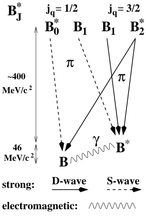
In the limit mQ → ∞, mesons composed of a heavy quark Q and a light quark q are charac- terised by the spin of the heavy quark, SQ, the total angular momentum of the light quark, jq =Sq+L, and the total angular momentum, J, where Sq and L denote spin and orbital an- gular momentum of the light quark, respectively. In the heavy quark limit, bothSQ and jq are good quantum numbers and the total angular momentum of the meson is given byJ =SQ+jq. ForL= 1, there are four states with spin-parityJP = 0+, 1+, 1+ and 2+. If the heavy quarkQ is a bottom quark, these states are labelled B∗0, B1 for both 1+ states1 and B∗2 [2], respectively.
The four states, commonly called B∗J, or alternatively B∗∗ 2, are grouped into two sets of de- generate doublets, corresponding to jq = 1/2 and jq = 3/2 as indicated in Table 1. Parity and angular momentum conservation put restrictions on the strong decays of these states to B(∗)π 3 (see Figure 1). The 0+ state can only decay to Bπ via an S-wave transition, the 1+1/2 to B∗π via an S-wave transition, the 1+3/2 to B∗π via a D-wave transition, and the 2+ state can decay to both Bπ and B∗π via D-wave transitions only. States decaying via an S-wave transition are expected to be much broader than the states decaying via a D-wave transition [3]. In addition to the single pion transitions, decays to B∗ππand Bππ are also possible. In the case of di-pion transitions, all four B∗J states are allowed to decay to B∗ as well as to B. Although these decays are phase-space suppressed, intermediate states with large width like B∗J → B(∗)ρ → B(∗)ππ may cause a significant enhancement of the B∗ππand Bππfinal states [4]. Additional B∗J decay modes with other than one or two accompanying pions are expected to be strongly suppressed but can not be excluded. Therefore, the notations B∗π(X) and Bπ(X) are chosen to refer to the final states of B∗J decays.
Given the HQET predictions listed in Table 1, the four B∗J states are expected to overlap in mass. So far, in analyses from LEP experiments [5–8] and from CDF [9] B∗J mesons are reconstructed in the Bπ final state only, observing one single peak in the Bπ mass spectrum.
This is not sufficient to resolve any substructure of the four expected B∗J states. In addition, for decays to B∗π where the photon in the decay B∗ →Bγ is not detected, the reconstructed Bπ mass is shifted byMB−MB∗ =−46 MeV/c2. A recent analysis [10] tries to cope with these problems by constraining all properties of the four B∗J states according to HQET predictions except for the masses and widths of B1(1/2) and B∗2.
In this paper a different approach is presented. Using information from the photon in the de- cay B∗ →Bγ, the B∗J →B∗π±(X) decays are statistically separated from the B∗J →Bπ±(X) de- cays. This allows a model-independent measurement of the branching ratio BR( B∗J →B∗π(X)).
Assuming that B(∗)πX decays produce small contributions to the B∗J width, this method gives insight into the decomposition of the B∗J into the states allowed to decay to Bπ (B∗0 and B∗2) from the other states that can only decay to B∗π.
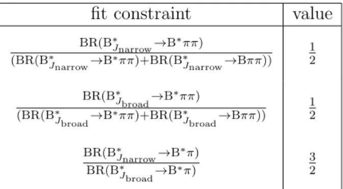
The Bπ invariant mass spectrum is also fit in the context of HQET expectations. This requires high statistics, extensive background studies and the tagging of the B∗ decay. Due to the complexity of the B∗J signal and its different decay modes, several constraints provided by
1In the limit mQ → ∞, the notations B1(1/2) and B1(3/2) are used. In the case of mixing of the J = 1 states, the notations B1(H) and B1(L) are used to distinguish the physical states.
2Throughout this paper, we use the Particle Data Group notation B∗J for orbitally-excited B mesons.
3Throughout this paper, B(∗)πdenotes the final states BπandB∗π. The notations B(∗)ππand B∗π(X) are to be interpreted in the same way.
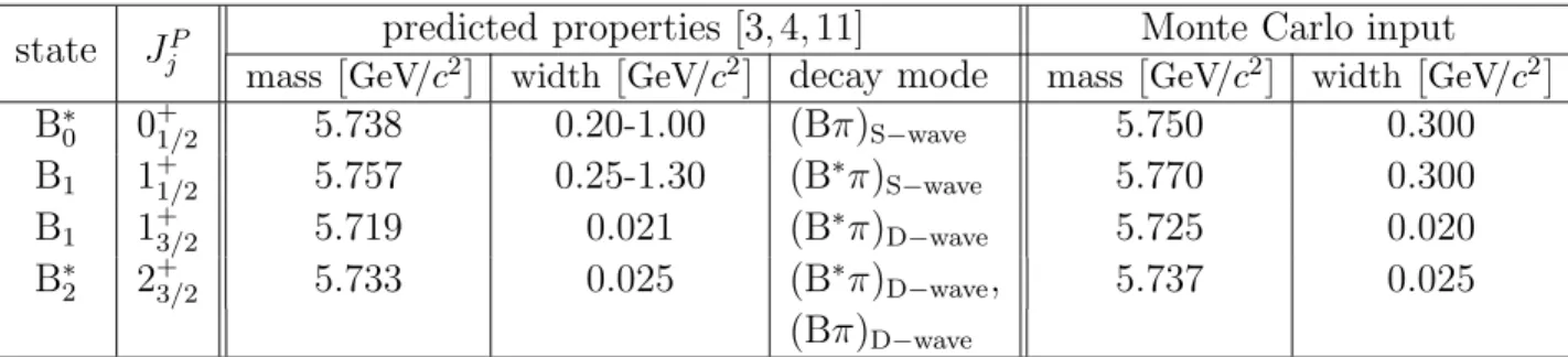
predicted properties [3, 4, 11] Monte Carlo input state JjP
massGeV/c2 widthGeV/c2 decay mode massGeV/c2 width GeV/c2 B∗0 0+1/2 5.738 0.20-1.00 (Bπ)S−wave 5.750 0.300 B1 1+1/2 5.757 0.25-1.30 (B∗π)S−wave 5.770 0.300
B1 1+3/2 5.719 0.021 (B∗π)D−wave 5.725 0.020
B∗2 2+3/2 5.733 0.025 (B∗π)D−wave, 5.737 0.025 (Bπ)D−wave
Table 1: Masses, widths and dominant decay modes based on theoretical predictions [3, 4, 11–
13] and the corresponding Monte Carlo input values used in the analysis. Recent calculations using a bag model predict widths of Γ(B∗0) = 0.141 GeV/c2 and Γ(B1(1/2)) = 0.139 GeV/c2 for the broad states [14].
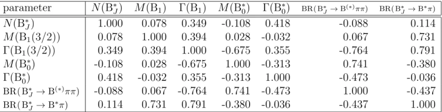
HQET are imposed. From the fitting procedure, we obtain model-dependent measurements of the mass and width of B1(3/2) as well as BR( B∗J →B∗π).
The paper is organised as follows: the next section describes the data sample and the event simulation. In Section 3, the analysis method is presented. The B reconstruction is described in Section 4. Section 5 contains the photon reconstruction. The pion reconstruction and the total Bπ mass spectrum are presented in Section 6. The BR( B∗J →B∗π(X)) measurement and results from a simultaneous fit to the Bπ± mass spectra of the samples enriched or depleted in the decay B∗J →B∗π±(X) are presented in Section 7. Systematic uncertainties are evaluated in Section 8. A discussion of the results and conclusions are given in Section 9.
2 Data sample and event simulation
The data used for this analysis were collected from e+e− collisions at LEP during 1991–1995, with centre-of-mass energies at and around the peak of the Z0 resonance. The data correspond to an integrated luminosity of about 140 pb−1. A detailed description of the OPAL detector can be found elsewhere [15, 16].
Hadronic events are selected as described in [17], giving a hadronic Z0 selection efficiency of (98.4±0.4) % and a background of less than 0.2 %. A data sample of about 4 million hadronic events is selected. Each event is divided into two hemispheres by the plane perpendicular to the thrust axis and containing the interaction point of the event. The thrust axis is calcu- lated using tracks and electromagnetic clusters not associated with any tracks. To select events within the fiducial acceptance of the silicon microvertex detector and the barrel electromag- netic calorimeter, the thrust axis direction4 is required to satisfy |cosθT| <0.8. Monte Carlo simulated samples of inclusive hadronic Z0 decays are used to evaluate efficiencies and back- grounds. The JETSET 7.4 parton shower Monte Carlo generator [18], with parameters tuned by OPAL [19] and with the fragmentation function of Peterson et al. [20] for heavy quarks is used to generate samples of approximately 10 million hadronic Z0decays, 2 million Z0→cc and 5 million Z0 →bb decays. The generated events are passed through a program that simulates the response of the OPAL detector [21] before applying the same reconstruction algorithms as
4 In the OPAL coordinate system, the xaxis points towards the centre of the LEP ring, the y axis points upwards and thezaxis points in the direction of the electron beam. θandφare the polar and azimuthal angles, and the origin is taken to be the centre of the detector.
for data. All generated Monte Carlo samples contain L = 1 states for bottom and charmed mesons, as well as vector meson partners of the ground states. The generated production rates, masses and widths of all resonant states are consistent with experimental measurements when available and with theoretical predictions elsewhere (see also Table 1).
3 Analysis overview
The analysis is based on the reconstruction of B∗ in the Bγ final state and a separate recon- struction of B∗J in the Bπ±final state. A direct reconstruction of B∗J decaying to B∗π, B∗ →Bγ giving Bγπ± in the final state is inappropriate because of the large combinatorial background and the insufficient detector resolution. Therefore, our approach employs a statistical separa- tion of B∗J →B∗π±(X) from B∗J →Bπ±(X) decays.
B mesons produced in Z0 →bb events are reconstructed inclusively to achieve high efficiency.
No attempt is made to reconstruct specific B decay channels. On the contrary, properties common to all weakly decaying b hadrons are used for the B reconstruction. For each B candidate, a weightW(B∗) is formed whereW(B∗) represents the probability for the B to have come from a B∗. The probability W(B∗) is based on the reconstruction of photon conversions and of photons detected in the electromagnetic calorimeter. All B candidates are then combined with charged pions to form B∗J meson candidates. Using the weight W(B∗), we derive two mutually exclusive subsamples of Bπ± combinations, one enriched and the other depleted in its B∗ content. Invariant Bπ± mass distributions are formed for both samples. The shape of the non-B∗J background of the two distributions is taken from Monte Carlo simulation and normalised to the data in the upper sideband region and subtracted from the corresponding data distributions. The branching ratio BR( B∗J →B∗π(X)) is obtained from the observed number of B∗J and the different efficiencies for B∗J →B∗π±(X) and B∗J →Bπ±(X) decays in the B∗-enriched and the B∗-depleted samples. Applying a simultaneous fit to the Bπ mass spectra of both samples several details of the B∗J four-state composition and of the B∗J decay modes are extracted.
Whereas the BR( B∗J →B∗π(X)) result obtained from counting the number of B∗J signal entries of the samples enriched or depleted in the decay B∗J →B∗π±(X) is model-independent and does not rely on the shape of the Bπ signal, the fit to the Bπ mass spectra makes use of HQET assumptions on the composition and the decay modes of the B∗J signal.
4 Selection and reconstruction of B mesons
B mesons are reconstructed using an extended version of the method used in earlier analyses [5, 22]. Since the reconstructed B mesons are used to form B∗ and B∗J candidates, the B reconstruction is tuned to minimise the uncertainties on the B direction and energy, while maintaining a high reconstruction efficiency.
4.1 Tagging of Z0 → bb events
To achieve optimal b-tagging performance, each event is forced to a 2-jet topology using the Durham jet-finding scheme [23]. In calculating the visible energies and momenta of the event and of individual jets, corrections are applied to prevent double counting of energy in the case of tracks with associated clusters [24]. A b-tagging algorithm is applied to each jet using three
independent methods: lifetime tag, highpT lepton tag and jet-shape tag. A detailed description of the algorithm can be found in [25]. The b-tagging discriminants calculated for each of the jets in the event are combined to yield an event b likelihoodBevent. For each event, Bevent >0.6 is required. After this cut, the Z0 →bb event purity is about 96%. The cut on the direction of the event thrust axis, |cosθT|<0.8, as described in Section 2, removes roughly a quarter of all Z0 →bb events and after the cut on Bevent, the total b event tagging efficiency with respect to all produced Z0 →bb events is about 49%, where these numbers are obtained from Monte Carlo simulation. At this stage, about 750 000 b hadron candidates are selected.
4.2 Reconstruction of B energy and direction
The primary event vertex is reconstructed using the tracks in the event constrained to the av- erage position and effective spread of the e+e−collision point. For the b hadron reconstruction, tracks and electromagnetic calorimeter clusters with no associated track are combined into jets using a cone algorithm [26] with a cone half-angle of 0.65 rad and a minimum jet energy of 5.0 GeV 5. The two most energetic jets of each event are assumed to contain the b hadrons.
For each jet we reconstruct the energy and direction.
In each hemisphere defined by the jet axis, a weight is assigned to each track and each cluster, where the weight corresponds to the probability that any one track or cluster is a product of the b hadron decay. The b hadron is reconstructed by summing the weighted momenta of the tracks and clusters. The reconstruction algorithm is applied to all b hadron species and is 100%
efficient. Since this analysis aims at the reconstruction of Bu,d mesons which make up about 80% of the b hadron sample, b hadron candidates are referred to as B mesons in the following.
Details of the reconstruction method are provided below.
4.2.1 Calculation of track weights
Two different types of weights are assigned to each track:
• ωvtx, calculated from the impact parameter significances of the track with respect to both the primary and secondary vertices;
• ωNN, the output of a neural network based on kinematics and track impact parameters with respect to the primary vertex.
The calculation of ωvtx requires the existence of a secondary vertex, whereas ωNN does not and is therefore available for all tracks. The search for detached secondary vertices proceeds as follows:
Each jet is searched for secondary vertices using a vertexing algorithm similar to that de- scribed in [5], making use of the tracking information in both the r−φ and r −z planes if available. If a secondary vertex is found, the primary vertex is re-fitted excluding the tracks assigned to the secondary vertex. Secondary vertex candidates are accepted and called ‘good’
secondary vertices if they contain at least three tracks and have a decay length greater than 0.2 mm. If there is more than one good secondary vertex attached to a jet, the vertex with the largest number of significant6 tracks is taken. If there is a tie, the secondary vertex with the
5The cone jet-finder provides the best b hadron energy and direction resolution compared to other jet finders studied here.
6A track is called significant if its impact parameter significance with respect to the primary vertex is larger than 2.5.
larger separation significance with respect to the primary vertex is taken. If a good secondary vertex is determined, a weight is calculated for each track in the hemisphere of the jet using the impact parameter significance of the track with respect to both the primary and secondary vertices. This weight is given by
ωvtx = R(b/η)
R(b/η) +R(d/σ) , (1)
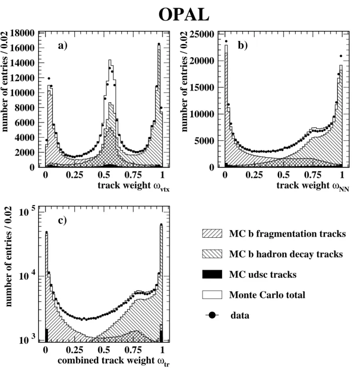
whereband ηare the impact parameter and its error with respect to the secondary vertex, and d andσ are the same quantities with respect to the primary vertex. R is a symmetric function describing the impact parameter significance distribution with respect to a fitted vertex. The ωvtx distribution for tracks of hemispheres with a good secondary vertex is shown in Figure 2a and compared with the corresponding Monte Carlo distribution. The weightωvtx shows a weak correlation with the momentum of the track.
For each track, the weight ωNNis calculated using an artificial neural network [27] trained to discriminate b hadron decay products from fragmentation tracks in a jet. The neural network was trained using as inputs the scaled track momentum xp = p/Ebeam, the track rapidity relative to the estimated B direction, the impact parameters of the track with respect to the primary vertex in the r −φ and r − z planes and the corresponding errors on the impact parameters [28]. As a preliminary estimate, the jet axis is taken as the estimated B direction.
TheωNN distribution is shown in Figure 2b. If a good secondary vertex exists, the track weight ωNN is combined with the vertex weight ωvtx using the prescription
ωtr= ωNN·ωvtx
(1−ωNN)·(1−ωvtx) +ωNN·ωvtx
. (2)
The weight ωtr in Equation 2 is approximately the probability that the track is a b hadron decay product. In the case where there is no good secondary vertex in the jet, the total track weight ωtr is simply given byωtr =ωNN. The combined weight ωtr for tracks of all hemispheres is shown in Figure 2c.
4.2.2 Calculation of cluster weights
Similar weights are calculated for energy clusters reconstructed in the electromagnetic and hadronic calorimeters to represent the probability the clusters came from a B hadron decay.
Weights ωecl and ωhcl are assigned to each electromagnetic and hadronic cluster in the hemi- sphere of the B meson based on their rapidity with respect to the estimated B direction. The weight is equal to the probability, calculated using the Monte Carlo simulation as a function of the cluster energy, that the cluster came from the decay of a B meson. Clusters associated with a track have the estimated energy of the track subtracted.
4.2.3 Calculation of B direction
The B momentum is calculated iteratively by a weighted sum of all tracks and clusters in the hemisphere:
~p=
Ntrack
X
i=1
ωtr,i·~pi+
Necal
X
i=1
ωecl,i·~pi+
Nhcal
X
i=1
ωhcl,i·~pi (3)
whereNtrack,NecalandNhcal denote the number of tracks, electromagnetic clusters and hadronic clusters, respectively. The rapidity calculation, for both tracks and clusters, is initially per-
formed relative to an estimate of the B meson direction7. The weights are then recalculated with the rapidity determined using the new B direction estimate.
An estimate of the B hadron direction is made for all B candidates based on the weighted momentum sum of the tracks and clusters in the jet. In addition, the vector from the primary vertex to the secondary vertex yields an estimate of the B direction for those jets where a good secondary vertex has been identified. When both estimates are available the weighted average is taken, using the calculated uncertainties of each direction estimate. The covariance matrices of the primary and secondary vertices determine the error on the B flight direction. The error on the momentum sum is estimated by removing each term in turn from the sum in Equation 3, calculating the change in the B direction caused by this omission and adding up in quadrature the corresponding error contributions from each track and cluster. The final estimate of the B direction is obtained by taking the error-weighted sum of the B direction calculated with the momentum sum method and the B direction obtained from the primary and secondary vertex positions. The direction information in the r−z plane of the secondary vertex is only used if the vertex is built with tracks that left at least four hits in thez-layers of the silicon microvertex detector (the maximum number of these hits per track is two).
The error ∆αon the weighted sum of both B direction estimators described in the previous paragraph is a measure for the quality of the B direction8. To improve the resolution on the B direction, which in turn dominates the Bπ mass resolution, a cut on ∆α is imposed. Since this analysis aims at a separation of some of the B∗J states by reconstructing different B∗J decay channels rather than obtaining a very good Bπ mass resolution, the cut ∆α <0.035 is rather loose. This cut removes the 20% of the B candidates with the poorest direction resolution, mainly those with no associated good secondary vertex.
4.2.4 Calculation of B energy
The resolution on the total energy of the B candidate can be significantly improved by con- straining the total centre-of-mass energy, ECM, to twice the LEP beam energy. Assuming a two-body decay of the Z0, we obtain:
EB = ECM2 −Mrecoil2 +MB2
2ECM , (4)
where the mass of the b hadron is set to the B meson mass MB = 5.279 GeV/c2 and Mrecoil
denotes the mass recoiling against the B meson. The recoil mass and the recoil energy Erecoil
are calculated by summing over all tracks and clusters9 of the event weighted by (1−ωi) and assuming the particle masses used in the calculation of Ei. To account for the amount of undetected energy mainly due to the presence of neutrinos, the recoil mass is scaled by the ratio of the expected energy in the recoil to the energy actually measured:
Mrecoil,new=Mrecoil,old· ECM−EB
Erecoil (5)
where EB is taken from Equation 4. The new recoil mass value Mrecoil,new obtained from Equation 5 is substituted into Equation 4 and the calculation of EB is iterated. After two
7 The initial input for this axis is the jet direction calculated using tracks and unassociated electromagnetic clusters.
8In the case where no good secondary vertex exists, ∆αis simply given by the uncertainty on the momentum sum.
9 Tracks and clusters not contained in the hemisphere of the B meson candidate have weightsωi = 0. ωi
denotes the weightωtr,i,ωecl,iandωhcl,ifor tracks, electromagnetic clusters and hadronic clusters, respectively.
iterations the uncertainty on the B meson energy is minimised. A minimum B energy of 15 GeV is required to further improve the energy resolution.
After all these cuts, the narrower Gaussian from a two Gaussian fit to the difference between the reconstructed and generated B meson energy has σ = 2.3 GeV, and 86% of the entries are contained within 3σ. The distribution of the difference between the reconstructed and generated φ angle of simulated B mesons can be described by a similar fit. The standard deviation of the narrower Gaussian is 14.2 mrad and 88% of the entries lie within 3σ. The corresponding quantities describing theθ resolution are σ = 15.0 mrad and 89%, respectively.
The complete B meson selection applied to the full data sample results in 574 288 tagged jets with a b purity of about 96%, as estimated from Monte Carlo. About 75% of the selected jets contain a good secondary vertex.
5 The decay B∗ → Bγ
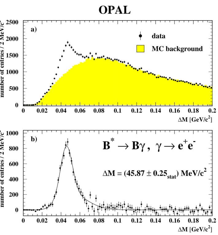
The photon produced in the decay B∗ →Bγ has an energy of about 46 MeV in the rest frame of the B∗. The mean energy of the photon in the laboratory frame is approximately 350 MeV, with a maximum energy below 800 MeV. Due to the kinematics of the process, these photons are produced predominantly in the core of the jet. The high particle density in this region gives rise to a high background level when identifying the photon. Since a high B∗ reconstruction efficiency is crucial for this analysis, photons are reconstructed in two ways: from energy deposits in the electromagnetic calorimeter and from converted photons in the tracking volume.
The conversion probability within the OPAL tracking system for photons coming from the decay B∗ →Bγ is approximately 8%.
5.1 Reconstruction of photon conversions
The reconstruction of converted photons is optimised for the low energy region. The selection algorithm is partially based on quantities that have been used in earlier analyses [29] but tuned to obtain high efficiency rather than very good angular and momentum resolution. Given the low energy carried by these photons, we ignore calorimetry information and only use tracking information for the reconstruction of converted photons.
Tracks with a total momentum pbelow 1.0 GeV/c, opposite charge assignment and a mea- sured dE/dxwithin three standard deviations of the expected value for electrons are combined into pairs. For each pair, the track with the greater scalar momentum is required to have a transverse momentum pt > 50 MeV/c with respect to the beam axis and at least 20 hits in the central jet chamber. For the track with lower momentum, a minimum pt of 20 MeV/c is required. The asymmetric selection cuts for the two tracks in a pair guarantee at least one well measured track and reflect the fact that the electron and the positron of a converted photon tend to have different momenta in the laboratory frame. To suppress random track combina- tions, the distance of closest approach between the two tracks of a pair in the r−φ plane has to be smaller than 1.0 cm with an opening angle between the tracks at their point of closest approach smaller than 1.0 rad.
In order to make optimal use of all the available information, the following measured quan- tities for each conversion track pair candidate are fed into a neural network:
• the distance of closest approach between the two tracks in the r−φ plane;
• the radial distance with respect to the z axis of the first and last measured hits in the inner tracking chambers for each track;
• the radial distance with respect to the z axis of the common vertex10 of both tracks obtained from a fit in ther−φ plane;
• the impact parameter with respect to the primary vertex in ther−φ plane of the recon- structed photon;
• the invariant mass of the track pair assuming both tracks to be electrons;
• the transverse momentum relative to the z axis of the lower momentum track.
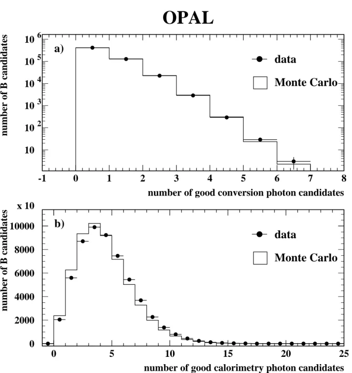
All conversion candidates with a neural network output greater than 0.7 and a photon energy below 1.5 GeV are called ‘good’ conversion candidates for a given B meson candidate if the opening angle between the reconstructed B momentum vector and the reconstructed photon momentum vector is smaller than 90◦. At this stage, an average of 0.82 good conversion candidates is selected per B candidate in both data and Monte Carlo. The candidate multiplicity distributions are shown in Figure 3a. The total efficiency to detect photons from the decay B∗ →Bγ with the conversion algorithm is estimated from simulation to be (2.70±0.01stat)%.
The efficiency is rather independent of the photon energy from 1.0 GeV down to 200 MeV where it rapidly drops to zero due to track selection requirements. The amount of fake conversions in the selected sample is estimated from Monte Carlo simulation to be (11.75±0.04stat)%.
Fits to the difference between the reconstructed and generated photon energy in Monte Carlo are made using the sum of two Gaussians, both constrained to the same mean value.
The narrower Gaussian has a standard deviation of 5 MeV at an energy of 200 MeV, and rises to 13 MeV at an energy of 750 MeV, and about 70% of the entries are contained within 3σ.
Similar fits to the φ and θ resolutions give values of 3.4 mrad (70%) and 5.4 mrad (61%), respectively.
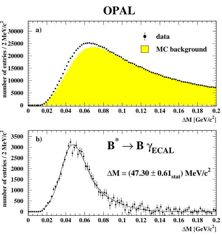
5.2 Reconstruction of photons in the electromagnetic calorimeter
Photons are also detected as showers in the barrel region of the electromagnetic calorimeter.
The location and energy of these showers are obtained from a fit to the energy deposits in the individual lead glass blocks not associated with any track. The whole reconstruction method has been shown to work in the dense environment of hadronic jets down to photon energies as low as 150 MeV. The details of the reconstruction are given in [30].
Showers in the electromagnetic calorimeter are accepted as photon candidates if they have an energy in the range 200 MeV to 850 MeV and a photon probability Pγ > 0.20, where Pγ
is the output of a simplified neural network [30]. If the opening angle between such a shower and a reconstructed B candidate is less than 90◦, this shower is considered a ‘good’ photon candidate for the corresponding B candidate. On average, there are 4.59 (4.38) good calorimeter photon candidates per B candidate selected in the data (Monte Carlo) sample. To correct for the observed discrepancy, the Monte Carlo is reweighted to the data distribution shown in Figure 3b. The efficiency to detect a photon from the decay B∗ →Bγ in the electromagnetic calorimeter is estimated to be (14.52±0.03stat)% using Monte Carlo simulated events. The fraction of fake photons arising from tracks and neutral hadrons in the sample ranges from
10Thezposition of this vertex is fitted independently and the reconstructed photon vector is constrained to thezcoordinate of the primary vertex to improve the accuracy of theθ determination.