Process Variants Using Clustering Techniques
Chen Li1, Manfred Reichert2, and Andreas Wombacher3
1 Information System group, University of Twente, The Netherlands lic@cs.utwente.nl
2 Institute of Databases and Information System, Ulm University, Germany manfred.reichert@uni-ulm.de
3 Database group, University of Twente, The Netherlands a.wombacher@utwente.nl
Abstract. In today’s dynamic business world, success of an enterprise increasingly depends on its ability to react to changes in a quick and flexible way. In response to this need, process-aware information systems (PAIS) emerged, which support the modeling, orchestration and mon- itoring of business processes and services respectively. Recently, a new generation of flexible PAIS was introduced, which additionally allows for dynamic process and service changes. This, in turn, has led to large number of process and service variants derived from the same model, but differs in structures due to the applied changes. This paper pro- vides a sophisticated approach which fosters learning from past process changes and allows for determining such process variants. As a result we obtain a generic process model for which the average distances between this model and the process variants becomes minimal. By adopting this generic process model in the PAIS, need for future process configuration and adaptation will decrease. The mining method proposed has been im- plemented in a powerful proof-of-concept prototype and further validated by a comparison between other process mining algorithms.
1 Introduction
In today’s dynamic business world, success of an enterprise increasingly de- pends on its ability to react to changes in its environment in a quick, flexible, and cost-effective way.Along this trend a variety of process and service support paradigms (e.g., service orchestration, service choreography, adaptive processes and services) and corresponding specification languages (e.g., WS-BPEL, WS- CDL, WSDL) have emerged. In addition, different approaches for flexible and adaptive processes exist [9, 28, 4]. Generally, process and service adaptations are not only needed for configuration purposes at build time, but also become nec- essary during runtime to deal with exceptional situations and changing needs;
i.e., for single instances of composite services and processes respectively, it must be possible to dynamically adapt their structure (i.e., to insert, delete or move
activities during runtime). In response to this need adaptive process manage- ment technology has emerged, which allows for such dynamic process and service changes [5].
The ability to adapt and configure process models at the different levels will result in a collection of model variants (i.e., configurations [1]). Such variants are created from the same process model, but slightly differing from each other.
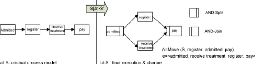
Fig. 1 depicts an example. The left hand side shows a high-level view on a patient treatment process as it is normally executed: a patient is admitted to a hospital, where he first registers, thenreceives treatment, and finallypays.
In emergency situations, however, it might become necessary to deviate from this model, e.g., by first starting treatment of the patient and allowing him to register later during treatment. To capture this behavior in the model of the respective process instance, we need to move activity receive treatment from its current position to a position parallel to activityregister. This leads to an (instance-specific) process model variant S0 as shown on the right hand side of Fig. 1. Generally, a large number of process model variants (process variants for short) derived from the same original process model might exist [24].
receive treatment Admitted
a) S: original process model b) S’: final execution & change
register pay
register
receive treatment
pay
AND-Split
AND-Join admitted
∆=Move (S, register, admitted, pay) S[∆>S’
e=<admitted, receive treatment, register, pay>
Fig. 1.Original Process Model S and Process Variant S’
In most approaches supporting the adaptation and configuration of process models each resulting process variant has to be maintained by its own, and even simple changes within a domain or organization (e.g. due to new laws or re-engineering efforts) might require manual re-editing of a large number of process variants. Over time this might lead to degeneration and divergence of the respective process models [3], which aggravates maintenance significantly.
Although some efforts on process flexibility have been made to make the process configuration and customization easier [9, 13, 4, 2].Our goal is to learn from the process changes applied in the past and to merge the resulting process variants into a generic process model which covers the existing process variants best. By adopting this generic process model within the PAIS, cost of change and need for future process adaptations will decrease.
Based on the two assumptions that: (1) process models are block-structured [9] and (2) all activities in a process model have unique labels, this paper deals with the following fundamental research question:
Given a set of process variants, how to derive a generic reference model out of them, such that the average distance between the reference model and the process variants becomes minimal?
The distance between two process models is measured by the number of change operations needed to transform one process model into another one.
Therefore, this figure can directly represent the effort for process adaptation and customization. (further explanation of distance is available in Section 2). Clearly, when the process variants are given, setting different model as the reference model would result in different average distance. The challenge is to find the best reference model, i.e. the one with minimal average distance to the process variants.
The reminder of this paper is organized as follows: Section 2 gives background information needed for understanding this paper. Section 3discusses major goals of process variants mining and shows why it is different from traditional process mining. In Section 4 we shows a method to represent a process model using a matrix called order matrix. After that, shows the algorithm to perform process varints mining at Section 5 and further validate the algorithm at Section 6.
We further extend it to handle mining with different activity set at Section 7.
The algorithm and prototype are afterwards given in Section 8.1. This paper concludes with a summary ad an outlook in Section 10.
2 Backgrounds
We first introduce basic notions needed in the following:process model, process change, process distance and bias andtrace.
Process Model LetP denote the set of all correct process models. A particular process modelS= (N, E, . . .)∈ Pis defined as a well-structured Activity Net [9].
N constitutes a set of activitiesaiand Eis a set of control edges linking them.
To limit the scope, we assume Activity Net to be block structured. Examples are provided by Fig 1.
Process change We assume that a process change is accomplished by applying a sequence of change operations to a given process modelS over time [9]. Such change operations modify the initial process model by altering the set of activities and/or their order relations. Thus, each application of a change operation results in a new process model. We define high-level change operations on a process model as follows:
Definition 1 (Process Change and Process Variant). Let P denote the set of possible process models and C the set of possible process changes. Let S, S0 ∈ P be two process models, let ∆ ∈ C be a process change, and let σ = h∆1, ∆2, . . . ∆ni ∈ C∗be a sequence of process changes performed on initial model S. Then:
– S[∆iS0 iff ∆ is applicable to S and S0 is the process model resulting from the application of∆ toS. We also denoteS0 as variant ofS.
– S[σiS0 iff∃ S1, S2, . . . Sn+1∈ P withS=S1,S0=Sn+1, andSi[∆iSi+1for i∈ {1, . . . n}.
Examples of high-level change operations includeinsert activity, delete ac- tivity, and move activity as implemented in the ADEPT change framework [9].
Whileinsert anddelete modify the set of activities in the process model,move changes the position of an activity and thus the structure of the process model.
For example, operation move(S,A, B, C) means to move activity A from its current position within process modelSto the position after activity Band be- fore activity C, while operation delete(S, A) expresses to delete activity A from process modelS. Issues concerning the correct use of these operations as well as formal pre- and post-conditions are described in [9]. Though the depicted change operations are discussed in relation to ADEPT, they are generic in the sense that they can be easily applied in connection with other process meta models as well [5]. For example, a process change as described in the ADEPT framework can be mapped to the concept of life-cycle inheritance as known from Petri Nets [10].
We refer to ADEPT in this paper since it covers by far most high-level change patterns and change support features when compared to other approaches [5].
Definition 2 (Bias and Distance). Let S, S0 ∈ P be two process models.
Then: The distanced(S,S0)betweenS andS0 corresponds to the minimal number of high-level change operations needed to transform process modelS into process model S0; i.e.,d(S,S0):=min{|σ| | σ ∈ C∗∧S[σiS0}. Furthermore, a sequence of change operationsσ with S[σiS0 and |σ|=d(S,S0) is denoted as bias between S andS0.
The distance between two process models S and S0 is the minimal number of change operations needed for transforming S into S0. The corresponding se- quence of change operations is denoted as bias between S and S0.4 Obviously, the shorter the distance between two process models, the more similar their control flow structure is. Generally, the distance between two process models measures the complexity for process model transformation or configuration. As example take Fig. 1. Here, the distance between S andS0 isone, since we only need to perform one change operationmove(S, receivetreatment, admitted, pay) to transform S into S0. In general, determining bias and distance between two process models is rather difficult. The complexity is atN P level [12]. We omit further details and refer to [12].
Here we use high-level change operations rather than change primitives (basic changes like adding/removing nodes and edges) to measure the distance between
4 Generally, it is possible to have more than one minimal set of change operations to realize the transformation from S into S0, i.e., given two process models S and S0 their bias is not necessarily unique. A detailed discussion of this issue is out of the scope of this paper since we are more interested in the change distance. We refer readers to [10, 12] for details.
process models. The reason is that using high-level change operations can guar- antee soundness and provide more meaningful measure of the distance. Due to the limited space, we omit the details are refer readers to [27].
Trace
Definition 3 (Trace). Let S = (N, E, . . .) ∈ P be a process model. We can define tas a trace of S iff:
– t≡< a1, a2, . . . , ak >, ai ∈N, be a sequence of activities, which is a valid and complete execution sequence based on the control flow in S. We define TS be a set which contains all the traces process modelS can produce.
– t(a≺b) is denoted as precedence relationship between activities a and b in tracet≡< a1, a2, . . . , ak>iff∃i < j :ai=a∧aj =b.
Here, we only consider traces composing ’real’ activities, but no events related to silent activities (i.e. activity nodes which contain no operation and exist only for control flow purpose). A detailed discussion about silent activity can be found in [12]. At this stage, we consider two process models as being the same if they aretrace equivalent, i.e.S≡S0 iffTS ≡ TS0. The stronger notion of bi-similarity [11] is not required in our context.
3 Mining Process Variants: Goals and Comparison with Process Mining
In this section, we first motivate the major goal behind mining process variants, namely to derive a reference process model out of a given collection of process variants. This shall be done in a way such that the different process variants can be efficiently configured out of the reference model. The letter is of particular importance if we want to learn from process instance deviations, derive an opti- mized process model from them, and migrate the already running instances to the newly derived model afterwards [28]. We measure the efforts for respective process configurations by the number of high-level change operations needed to transform the reference model into the respective model variant. The challenge is to find a reference model such that the average number of change operations needed (i.e., the average distance) becomes minimal.
To make this more clear, we compare process variants mining with traditional process mining. Process mining based on execution log has been researched inten- sively during the past few years [6]. An overview on existing techniques is given in [16]. In a nutshell, these approaches are trying to discover the underlining pro- cess model from execution logs which typically record the starting/completion events of each process activities. Obviously, input data for process and process variants mining differ. While traditional process mining operates on execution logs, mining of process variants is based on change logs (or the process variants we can obtain from them). Of course, such high-level consideration is insufficient
to prove that existing mining techniques do not provide optimal results with re- spect to the above goal. In principle, methods like alpha algorithm or genetic mining can be applied to our problem as well. For example, we could derive all traces producible by a given collection of process variants [15] and then apply existing mining algorithms to them. Or, if there are enough instances for each process model variant, we can mine their traces to discover a corresponding pro- cess model. To make the difference between process and process variants mining more evident, in the following, we consider behavioral similarity between two process models as well as structural similarity based on their bias.
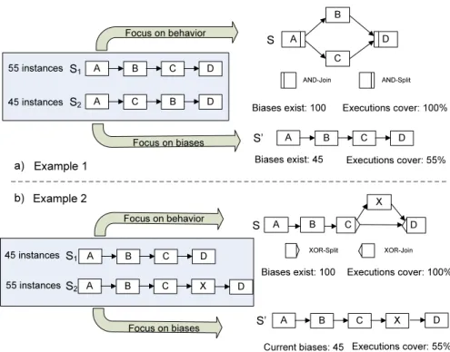
The behavior of a process modelS can be represented by the set of traces TS it can produce (c.f. Def. 3). Therefore, two process models can be compared based on the difference between their trace sets [6, 15, 16]. By contrast, biases can be used to express the (structural) distance between two process models, i.e., the minimal number of high-level change operations needed to transform one model into the other [12]. While the mining of process variants addresses structural similarity, traditional process mining focuses on behavior. Obviously, this leads to different choices in algorithm design and also suggest different mining results.
Fig. 2 shows two examples.
Example 1 Example 2
A B C D
A B C X D
C D
A
X Focus on behavior B
Focus on biases S1
S2 45 instances
55 instances
S
S’
Current biases: 45
A B C D
A C B D
S1
S2
A B C D
Focus on behavior
Focus on biases 55 instances
45 instances
A D
B
C S
S’
Biases exist: 100 Executions cover: 100%
Biases exist: 45 Executions cover: 55%
Biases exist: 100 Executions cover: 100%
Executions cover: 55%
A B C X D
AND-Split AND-Join
XOR-Split XOR-Join
a) b)
Fig. 2.Mining focusing either on Behavior or on Minimization of Biases
Consider Example 1 (c.f. Fig. 2a)) which shows two process variantsS1 and S2. Assume that 55 process instances are running onS1and 45 instances onS2. We want to derive a reference process model such that the efforts for configuring the 100 process instances out of the reference model become minimal. If we focus on behavior, like existing process mining algorithms do, the discovered process model will have a structure likeS; all traces producible onS1andS2respectively can be produced onS as well, i.e.TS1 ⊆ TS andTS2 ⊆ TS. However, if we adopt Sas reference model and relink instances to it, all instances running eonS1orS2
will have a non-empty bias. The average weighted distance betweenS andS1(S andS2) isone; i.e., for each process instance we need on average one high-level change operation to configureS intoS1 andS2 respectively. More precisely, we would need to move either B or Cin S to either obtain S1 or S2; i.e., S[σ1iS1
withσ1=move(S,B,A,C) (c.f. Def. 1 for detail parameterization) and S[σ2iS2 withσ2=move(S,B,C,D). We describe a method to compute biases in [12].
By contrast, if the goal is to reduce the average bias between reference model and process (instance) variants, we should chooseS0as reference model. Though S0 does not cover all tracesS1 andS2 can produce (i.e.,TS2 *TS0) the average distance between reference model and process instances becomes minimal with this approach. More precisely, the average distance between S0 and instances running either onS1orS2corresponds to0.45; i.e., while no adaptations become necessary for the 55 instances running onS1, we need to move activityBfor the 45 instances based on S2, i.e. S0[σ0iS2 with σ0 =move(S0,B,C,D). Though S0 cannot cover all traces process variants S1 and S2 can produce, adapting S0 rather thanSas the new reference process model requires less efforts for process configuration, since the average weighted distance betweenS0 and the instances running on bothS1 andS2 is 55% lower than when usingS.
Regarding Example 2 (c.f. Fig. 2), activityXis only present inS2, but not in S1. When applying traditional process mining, we obtain process modelS(with X being contained in a conditional branch). If focus is on minimizing average change distance,S0will have to be chosen as reference model. Note that in Fig. 2 we have chosen rather simple process models to illustrate basic ideas. Of course, our approach works for process models with more complex structure as well, see Sec. 5.
Our discussions on the difference between behavioral and structural simi- larity also demonstrate that current process mining algorithms do not consider structural similarity based on bias and change distance (we will quantitatively compare our mining approach with existing algorithms in Section 5). First, a fundamental requirement for traditional process mining concerns the availabil- ity of a critical number of instance traces. An alternative method is to enumerate all the traces the process variants can produce (if it is finite) to represent the process model, and to use these traces as input source for process mining algo- rithms based on process logs. Unfortunately, this does also not satisfy our need on reducing biases since it focuses on covering execution behavior as captured in execution log (recall Example 1 and 2). Clearly, enumerating all the traces would be also a tedious and expensive job. For example, if an AND-split and
AND-join block contains five branches and each branch contains five activities, the number of traces for such a structure is (5×5)!/(5!)5= 623360743125120.
4 Represent Process Model Logic as an Order Matrix
After showing the goal for process variant mining, we start describing the ap- proach to perform the mining. The theoretical backgrounds of high-level change operations have been discussed in ADEPT technique which is based on WSM net [9], and life-cycle inheritance which is based on Petri net [10]. One key feature of our ADEPT change framework is to maintain the structure of the unchanged parts of a process model [9]. For example, if we delete an activity, this will neither influence the successors nor the predecessors of this activity, and also not their control relationships. To incorporate this feature in our approach, rather than only looking at direct predecessor-successor relationships between two activities (i.e. control flow edges), we consider the transitive control dependencies between all pairs of activities; i.e. for every pair of activities ai, aj ∈NT
N0, ai 6= aj, their execution order compared to each other is examined. Logically, we check the execution orders by considering all traces a process model can produce (c.f.
Sec. 2). Results can be formally described in a matrixAn×n withn=|NT N0|.
Four types of control relations can be identified (cf. Def. 4):
Definition 4 (Order matrix). Let S = (N, E, . . .) ∈ P be a process model with N ={a1, a2, . . . , an}. Let furtherTS denote the set of all traces producible on S. Then: Matrix An×n is called order matrix of S with Aij representing the relation between different activitiesai,aj∈N iff:
– Aij = ’1’ iff (∀t∈ TS with ai, aj∈t⇒t(ai ≺aj))
If for all traces containing activitiesai andaj,ai always appears BEFORE aj, we denote Aij as ’1’, i.e.,ai is predecessor of aj in the flow of control.
– Aij = ’0’ iff (∀t∈ TS with ai, aj∈t⇒t(aj ≺ai))
If for all traces containing activityai andaj,aialways appears AFTERaj, then we denoteAij as a ’0’, i.e. ai is successor ofaj in the flow of control.
– Aij = ’*’ iff (∃t1 ∈ TS, with ai, aj ∈ t1∧t1(ai ≺ aj)) ∧ (∃t2 ∈ TS, with ai, aj∈t2∧t2(aj≺ai))
If there exists at least one trace in which ai appears before aj and at least one other trace in which ai appears after aj, we denote Aij as ’*’, i.e. ai
andaj are contained in different parallel branches.
– Aij = ’-’ iff (¬∃t∈ TS :ai∈t∧aj ∈t)
If there is no trace containing both activityai andaj, we denote Aij as ’-’, i.e.ai andaj are contained in different branches of a conditional branching.
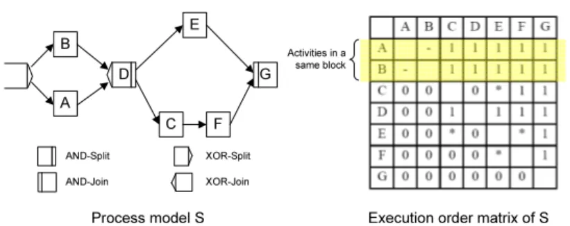
Figure 3 shows an example. Besides control flow edges which shows direct predecessor-successor relationship, process model S also contains four types of control flows: AND-Split, AND-Join, XOR-Split and XOR-join. The order ma- trix can represent all these relationship in the matrix. For example activity A and activity Bwould never appear in one trace since they are in two different
A
C B
E
F G D
Process model S Execution order matrix of S Activities in a
same block
AND-Split AND-Join
XOR-Split XOR-Join
Fig. 3.Order matrix for process modelS
branches of an XOR block. It is denoted as ’-’ in the matrix at Aab and Aba. Similarly, we can denote all the execution orders between every pair of activ- ities. The main diagonal in the matrix is empty since we do not compare an activity with itself. As one can see, elements Aij and Aji can be derived from each other. If activity ai is a predecessor of activity aj, (i.e. Aij = 1), we can always conclude that Aji = 0 holds. Similarly, if Aij ∈ {’*’,’-’}, then we will obtainAji=Aij. Please note that order matrix is different from the adjacency matrix as used in graph theory [18]. The reasons include that it differentiates AND and XOR block, does not contain unnecessary silent activities, and handle loop differently [12].
Under certain constraints, an order matrix A can uniquely represent the process model, based on which it was built on. This is stated by Theorem 1.
Before giving this theorem, we need to define the notion ofsubstring of trace: Definition 5 (Substring of trace). Lett andt0 be two traces. We define tis a sub-string of t0 iff [∀ai, aj ∈ t, t(ai ≺ aj) ⇒ ai, aj ∈ t0∧t0(ai ≺aj)] and [∃ak∈N:ak ∈/ t∧ak∈t0].
Theorem 1. Let S, S0 ∈ P be two process models, with same set of activities N = {a1, a2, . . . , an}. Let further TS, TS0 be the related trace sets and An×n, A0n×n be the order matrices ofS andS0. ThenS6=S0 ⇔A6=A0, if (¬∃t1, t01∈ TS:t1 is a substring oft01) and (¬∃t2, t02∈ TS0:t2 is a substring oft02).
According to Theorem 1, there is a one-to-one mapping between a process model S and its order matrixA, if the substring constraint is met. A proof of Theorem 1 can be found in [12]. The substring constraint is also not very strong since we can easily detect and handle it [12]. Thus, analyzing order matrix (cf.
Def. 4) would be sufficient for analyzing a process model, since an order matrix can uniquely represent the process model.
The order matrix can also help on determining blocks: if the internal execu- tion orders of the activities in the same block are ignored, these activities should have the same execution orders to the rest of activities. Take the order matrix in Fig. 3 for example. If we ignore the internal relationship between activities Aand B, the execution orders betweenAand the rest of activities are the same
as the execution orders between B and the rest of activities (as marked up in yellow in Fig. 3, the first two rows are the same if we ignore the execution order betweenAandB). Therefore, without knowing the process model, we can already determine a block with activitiesAandB, which are in different branches of an XOR block.
We therefore can apply the similar idea on designing the mining algorithm.
When two activities have the same or similar execution orders to the rest of activities, we therefore can cluster them together as a block. And if we repeat it again and again, then activities will form a small blocks, and small blocks will form bigger ones, and we can therefore mine a process model out by clustering activities or blocks. The following sections will give a detail explanation of our method.
5 Discovering Generic Process Reference Model
The goal of this paper is to mine the process variants in order to derive a new reference model which is easier configurable. Since we restrict ourselves on han- dling block-structured process models, we can build a process model by enlarging blocks, i.e. some activities can form blocks, and the block is enlarged by merging other blocks. If all the activities and blocks are linked together, we therefore can get a process model which represent the new reference process models.
Therefore, our general approach for mining process variants is as follows:
1. Represent process variants by a Type-level Order Matrix (Section 5.1).
2. Determine which activities should be clustered together to form a block, based on the type-level order matrix. (Section 5.3).
3. Make respective change of the type-level order matrix after building a block in step 2 (Section 5.4).
4. Repeat 2,3 until all activities (blocks) are clustered together.
5. Evaluation the fitness of the resulting process model (Section 5.5).
An illustrative example is given in Fig. 4. It contains five process variants Si∈ P,i=∞,∈, . . .5as well as the weight of each variance based on number of execution. In our example, 30% of instances were executed according to process variantS1, while 15% instance according to variantS2. In another scenario, for example, when we only have the process variants derived from the same reference model, but no information about the instance executions, we can assume the variants are un-weighted. i.e. every process variant will have the same weight 1/n, wherenis the number of process variants in the system. So far, our example is given based on the assumption that each process variant has the same activity set. See Sec. 7 for a relaxation of this constraint.
5.1 Type-level Order Matrix
When given a set of process variants, we first need to compute the order matrices for these process variants. To our case, we need to draw five order matrices
S1: 30%
S2: 15%
S3: 20%
S4: 20%
S5: 15%
B C
E
A D
D
A C B E
A
D E
B C
B E
A
C
D
A E
B
C
D
Weight of process variant, based on number of executions Fig. 4.Illustrative example for our mining approach
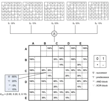
according the five process variants in the system (c.f. Fig. 5). Afterwards, we can analyze the execution orders between every pair of activities shown in different order matrices. As the execution order between two activities may not be unique in all order matrices, this is not a fixed relationship but a distribution value of the four types of execution orders. For example, activity C is 65% successor of activity B (as in S1, S2, S4), 20% predecessor of B (as in S3) and 15% in different XOR-split branching with B (as in S5). We therefore can define the execution order between two activities a and b, as a four dimensional vector, Vab = (vab0, vab1, vab∗, vab−), which corresponds to the frequency of the four types of execution orders (’0’, ’1’, ’*’, ’-’) as specified in Def. 4. For example, vCB1shows the percentage where activitiesC, Bhave relationship ’1’, i.e. activity C is a predecessor of B. Clearly, vab0+vab1+vab∗ +vab− = 1. To our case, VCB = (0.65,0.2,0,0.15).
We can formally define a type-level order matrix as follows:
Definition 6 (Type-level Order Matrix).
Let Si = (Ni, . . .) ∈ P, i = (1,2, . . . , n) be a set of process variants. Ai
is the order matrix for Si and wi represents the number of instances executed according toSi. The Type-level Order Matrix for the process models is defined as a 3-dimensional matrixVm×mwithm=|S
Ni|andVjk= (vjk0, vjk1, vjk∗, vjk−) being a four dimensional vector.vjk0=P
i=(1,...,n),Aijk=000wi/P
i=(1,...,n)wifor
∀Si∈ P :aj, ak ∈Ni∧j6=k. Similarly we can computevjk1, vjk∗ andvjk−. In a type-level order matrix, Vjk shows the percentage value of the four types of execution orders in all the process models containing activity aj and ak (j 6=k). Please note that we do not necessarily constrain all process models to have the same activity set. We will further describe how we handle such situation in Section 7. To our example, the type-level order matrix V for the process variants shown in Fig. 4 is depicted in Fig. 5.
In the type level order matrix, the main diagonal is empty since we do not specify the execution order between an activity and itself. For the rest of ele- ments, when the value in a certain dimension is empty, it means it is 0.
0 1
* -
‘0’ : successor
‘1’ : predecessor
‘*’ : AND-block
‘-’ : XOR-block
S1: 30% S2: 15% S3: 20% S4: 20% S5: 15%
V
VCB= (0.65, 0.20, 0, 0.15)
‘0’ : 65%
‘1’ : 20%
‘*’ : 0%
‘-’ : 15%
Fig. 5.Type-level order matrix
In Sec. 4, we have shown that we can use order matrix to determine blocks in a process model. i.e. two activities can be clustered together to form a block if the execution order between them and the rest of activities are same (c.f. Sec.
4). Similar idea can be applied, when analyzing type-level order matrix. The following sections will describe the methods in details.
5.2 Two Measures for Block Detection: Cohesion and Separation A naive approach would be to make an order matrix based on the type-level order matrix by setting the execution orders to the one with the highest frequency in the vector. For example, because VCB = (0.65,0.2,0,0.15) the execution order of C, B should be successor, sinceVAB0is 0.65 which is the highest among the four. If we apply it to every pair of execution order, we can then generate an
’order matrix’, based on which we can build one process model. Unfortunately it will not work, since an ’order matrix’ determined in this way does not necessarily represent a valid process model. Take the order matrix in Fig. 3 for example, if we changeAAE from 1 to 0, there would be no process model representing such order matrix. This has triggered us to think of other methods.
As described in the general process at the beginning of this section, whenever we need to determine a block, we need to know which activities (blocks) should be in such block, and what execution order should the activities in the blocks
be? In this section, we will introduce two measures:cohesion andseparation as the answer of these two questions.
Before we define cohesion and separation, we first need to define a function f(α, β) which shows the closeness between two vectors α= (x1, x2, ..., xn) and β = (y1, y2, ..., yn):
f(α, β) = α·β
|α| × |β| =
Pi=n
i=1xiyi
qPi=n
i=1x2i ×qPi=n
i=1y2i
f(α, β) computes the cosine value of the angleθbetween the two vectorsα, β in an Euclid space. The value range of if this function is [0,1] where 1 means two vectorα, βprecisely match in their directions and 0 when they are precisely vertical.
Cohesion Cohesion measures how closely related the objects in a cluster are.
In our context: it indicates how strong the relationship between two activities is.
In the type level order matrix, if, for instance, we decide to cluster activityB andEtogether to form a block, the relationship between the two activitiesB, E in the block, is determined by the vectorVBE. This vector shows the execution order betweenBandE. We then can compareVBE with the four benchmarking vectors (which corresponding to the four axes in the four-dimensional space):
V0= (1,0,0,0), V1= (0,1,0,0),V∗= (0,0,1,0),V0= (0,0,0,1). To which of the four axes VBE is closest, we can define it as the execution order betweenBand E. And the credibility is therefore determined by the cosine value between these two vectors. For example, VBE = (0,0.7,0.3,0), so the closest vector is V1, and the closeness which is evaluated by the cosine value equals 0.919.
Since cohesion is determined by angle between a vector and its closest axis, the value range of the cohesion value is not [0,1] but to some degree smaller.
We can also normalize cohesion to a value between 0 and 1. It is not difficult to find that when a vector equals to (0.25,0.25,0.25,0.25), the cohesion equals to the minimal one which is 0.5. Therefore the cluster cohesion, which shows the credibility of the relationship between the two activities (blocks) in a block, equals:
Cohesion(A, B) = 2×max(f(VAB, V0), f(VAB, V1), f(VAB, V∗), f(VAB, V−))−1 In this way, we can determine and measure the internal relationship between two activities (blocks) by a value between 0 to 1. Regarding to the example given above,Cohesion(B,E) therefore equals 0.838, and the execution order between activitiesB,Eispredecessor.
Separation Separation measures how distinct or well-separated a cluster is from other clusters. In our context, we indicate how well two activities (blocks) are suited to be clustered together, i.e. to form a block.
This factor Seperation(A, B) is determined by how similar the execution orders of activity AandBwhen compared with the rest of activities. As to our case shown in Fig. 4,Seperation(A, B) is determined by the closeness (measured by the cosine value) off(VAC, VBC),f(VAD, VBD) andf(VAE, VBE). Therefore, we can define cluster separation equals:
Separation(A, B) = P
x∈N\{A,B}f2(VAx, VBx)
|N| −2
In the formula of separation,N is the set of activities. The reason to square the cosine value is to emphasize the differences between the two compared vec- tors, like most clustering algorithms do [14]. And dividing the formula by|N|−2 can normalize the value to a range between [0, 1]. As to our example in Fig. 4, Seperation(A, B) = 0.905.
5.3 Detecting Activities to Form a Block
After introducing Cohesion and Separation in Section 5.2, we can apply these two measures to determine: which two activities should be clustered together, and what the relationship between them should be.
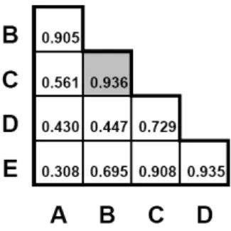
The idea is similar to Agglomerative Hierarchical Clustering as introduced in the field of data ming [14]. Similar to clustering algorithm in data ming which measures the distance between each pair of nodes in a dataset, we measure the distance between each activity pair by computing the separation value between them. The higher the separation value is, the more likely two activities tend to be clustered together. Regarding to our case in Fig. 4, the separation values between every pair of activities are shown in Fig. 6. We denote this table as separation table.
Fig. 6.The separation table of the type-level order matrix in Fig. 5
Regarding the separation table, it becomes clear that activityBandChave the highest separation value (marked up in grey). To be more precise, the sep- aration between B and C is 0.936. Since it is the highest one, we can already
determine the activities in our first block: activityBandC. However, when deal- ing with complex examples, there can several maximal separation values. For this case, we also need to compute the cohesion between the pairs with the highest separation values. The pair with highest cohesion shall be selected, since the re- lationship of the two activities (measured by the cohesion) is most significant. If separation and cohesion are both the same for two blocks, we do not differentiate which one should be first.
After we determined the activities to form a block, we need to determine which execution order should activityBandChave, as well as the cohesion value which indicates how strong the relationship is (c.f. Cohesion).Cohesion(B, C) = 0.867, and the closest axis isV1 which identifies that activityBis a predecessor of activity C.
5.4 Re-compute the Type-level Order Matrix
After we cluster activities Band C, we need to decide the relationship between this new block and the result of activities. In the traditional clustering tech- niques, the distance (separation, as to our case) between this block and the node out side this block is either the maximal, or the minimal or the average of the distances between that node and the nodes in the cluster [14]. For ex- ample, according to Agglomerative hierarchical clustering [14], after activitiesB and Care clustered together, the distance (separation) between this block and another activity (e.g.A) is either the minimal (0.561) or the maximal (0.905) or the average (0.733) of separation(A,B) = 0.905 and separation(A,C) = 0.561.
Unfortunately, such technique will not work in our context because we do not simply consider each activity as a high dimensional vector. When two activities are clustered together, we actually moved the positions of the activities in the process variants so that they could be linked together to form a block. There- fore, rather than simply modify the separation values, we need to re-compute the execution orders between the activities in the block and the activities out- side the block. We do it by compute the means. For example, activityBis 100%
predecessor of D, while activity C is 15% successor, 65% predecessor and 20%
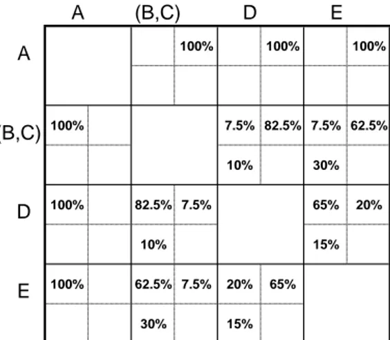
AND-Split withC(c.f. Fig. 5). After we cluster activityBand C, the execution order of block (B,C) to activityD, turn to be 7.5% successor, 82.5% predecessor and 10% AND-split. We can formally describe it as follows: after activity a, b are clustered together, the new type-level order matrixV(n−1)×(n−1)0 equals:
1. V(a,b)x0 = 1/2(Vax+Vbx) andVx(a,b)0 = 1/2(Vxa+Vxb) for all x∈N\ {a, b}
2. Vxy0 =Vxy for allx, y∈N\ {a, b}
The new type-level order matrixV0after clustering activityBandCis shown in Fig. 7.
5.5 Mining Result and Evaluation
After we get a new type-level order matrix, we can repeat the following two pro- cess as described in Section 5.3 and Section 5.4, i.e. first determine the activities
A (B,C) D E
A 100% 100% 100%
(B,C) 100% 7.5% 82.5% 7.5% 62.5%
10% 30%
D 100% 82.5% 7.5% 65% 20%
10% 15%
E 100% 62.5% 7.5% 20% 65%
30% 15%
Fig. 7.The new type-level order matrix after clusteringBandC
(blocks) to be cluster together, and then re-compute the type-level order matrix.
The iteration will continue until all activities and blocks are clustered together (the number of iteration equals the number of activities minus two). The final result after all iteration is shown in Fig. 8.
Figure 8 shows the process modelS0 we mined out. The result does not only show a process model, but also shows how the process model been built up in each iteration ( shown as a number at the right-bottom corner of each block) and what the credibility of the control flow is. For example, the credibility of the successor relationship between activityEand block with activityCandDis 0.792, which is relatively low when compared to the other control flows. It reflects that:
based on the instances described in Fig. 4, the relationship between activity C andEhas been configured more than others. And the credibility of activityCis a predecessor of activityEis not very strong.
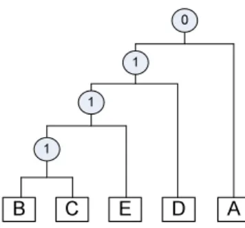
Since we follow a strict block structure so far, the result can also be visualized in an expression tree as proposed in [25]. Similar tree structure can also be found in hierarchical clustering algorithm [14]. The tree structure of the process model in Fig. 8 is depicted in Fig. 9.
0.867
B C 0.792 E 0.939 D
A 1.0
1 2
3 4
Fig. 8.The resulting process modelS0
A
B C E D
1 1
1 0
Fig. 9.The binary tree representation of process modelS0
The rectangle in Fig. 9 represents the activities and the circle in the root rep- resents the execution order. The execution order shows the relationship between the left subtree and the right sub tree. For example, the relationship between activity BandCis 1, which meansBis a predecessor of C. The tree can grow as the blocks grow in our algorithm. Whenever a block is created, the new activities being included in the block will become the new right subtree of old one. For example, after activityBandCare clustered with the relationship of predecessor, the existing tree has two subtreesBandCand a root with execution order ”1”.
After the first iteration, the algorithm decided to cluster the block withBandC with the activityE. The new activity will then be listed as the right subtree of the new tree with the execution order of ”1” shown on the root.
If we perform an inorder traversal (details is available in [25]) of the tree, we can also represent the process model in a linear structure like an arithmetic expression. For this case the expression is:(((B 1 C) 1 E) 1 D) 0 A). In this expression, 0,1 represent the execution order just like ”+” ”-” in arithmetics.
ThereforeB 1 Cmeans activityBis a predecessor of C.
5.6 Two Evaluation Measures
Besides the cohesion which evaluate the local fitness of a certain block, we can also define global evaluation measures which show the ”goodness” of the process model we mined out. The measures include: accuracy andprecision.
We first can build an order matrixA0 based on the process modelS0 which we mined out (c.f. Fig. 8). After that, we can also build a type-level order matrix V0 only based onA0. For instance, ifA0ij = 0, then the corresponding element in the type-level order matrix is a vectorVij0 = (1,0,0,0). Or, ifA0ij = 1, we can determine the vector to be Vij0 = (0,1,0,0). Based on the comparison between the type-level order matrixV (c.f. Section 5.1) andV0, theaccuracyandprecision can be defined as follow:
Accuracy(S0) = P
ai,aj∈N,i6=j,Vij=V0ij1
|N| ×(|N| −1)
Accuracy(S’)measures how accurate the mined out process modelS0 is when compared to the process variants. It is determined by how many execution or-
ders have been perfectly satisfied compared with all the activities pairs. We define two vectors Vij and Vij0 perfectly match if Vij = Vij0. To our example, 10 execution orders satisfy this relationship out of 20 activity pairs. Therefore, Accuracy(S0) = 0.5.
P recision(S0) = P
i,j∈N,i6=j,f(Vij6=V0ij)f2(Vij, Vij0) P
i,j∈N,i6=j,Vij6=V0ij1
Precision(S’) shows how precise the execution orders in S0 are when com- pared to the process variants in the system. When computing the precision, only the none-perfect match cases are counted. Precision(S0) equals the average square of the similarities (measured by the f function in Section 5.2) between the none-perfect match element inV andV0. We define two vectors Vij andVij0 not perfectly match if Vij 6= Vij0. The reason to square the cosine measure is to emphasize the different, as most data mining measures do [14]. In our case, precision(S0) = 0.837.
Clearly, a more precise way to evaluate the resulting model is to really com- pute the distances between the mined model and the process variants. However, as computing the distance between two given process models is at N P level [12], it is not very sufficient to do so. Therefore, we introduce the two measures accuracy andprecision to give an approximate result. In the following section, we will also compare these two different methods for measuring the goodness of the resulting model.
6 Validation
The complexity of the process variants mining algorithm described above is O(n3). Like other clustering algorithms in data mining [14], this algorithm is trying to solve a complex combinatory optimization problem in polynomial time.
This leads to the benefit that it can solve a problem with large scale, as well as the disadvantage that it only searches for local optimal but not global optimal.
Therefore, it is not possible to systematically prove that the algorithm really does what we want, i.e. reduce the number of biases in the system by improving the reference process model.
However, we can compare the process model we mined out with some other models. The comparison is based on: how many biases would exist in the system if we set different models as the new reference process model. To emphasize again, the biases are evaluated by the number change operations need to transform the reference model to the variants. It is also same to the largest common divider as defined in [13] i.e., how many activities we need to remove from the process variants to make it as a life-cycle inheritance of the reference process model [10].
For example, if we compare the eS1 in Fig. 4 with the process model S0 as we mined out in Fig. 8. We only need to moveone activity Eto the position after Cand beforeD(i.e.move(S1,E, C, D) in ADEPT [9]) in order to transformS1
to S0. If we apply the life-cycle inheritance as Aalst defined in Petri-net world
[13, 10] we only need to remove activityEinS1 so thatS1could be an life-cycle inheritance process model of S0. In this way, we can define that if we set the process modelS0 as the new process template, there is only one bias existing in each instance running according to process model S1. By applying the similar technique, we can compute the biases in other variants if we setS0 as the new type level order matrix.
There are two groups of process models that can be the candidates for the new reference process model. The first group contains all the process models we already know. Clearly, the five process variants S1, S2, S3, S4, S5 shown in Fig.
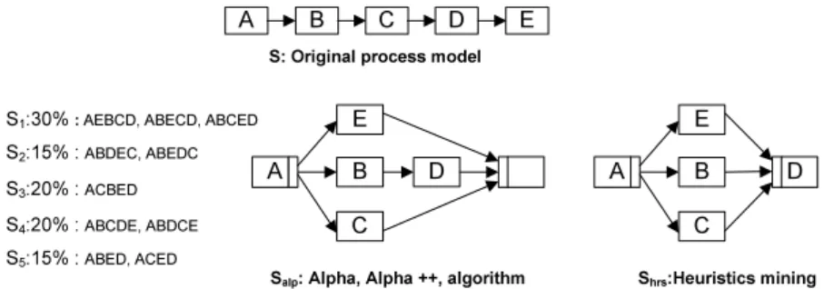
4 belong to this group. In addition, we can also assume that there exists an original reference process model. Lets assume it isS in Fig. 10. Comparing these existing models with the one we obtained through our approach, for example, already shows that it will be not sufficient to simply set the reference model to the most frequently used process variant (S1 in our example).
Salp: Alpha, Alpha ++, algorithm A
E
C
B D A D
E
C B
Shrs:Heuristics mining
A B C D E
S: Original process model
S1:30% : AEBCD, ABECD, ABCED S2:15% : ABDEC, ABEDC S3:20% : ACBED S4:20% : ABCDE, ABDCE S5:15% : ABED, ACED
Fig. 10.The candidate process models
The second group of process models includes the process models that we discovered using different algorithms. Clearly, the process modelS0 from Fig. 8, as obtained using our process variants algorithm is in this group. In addition, we can compare the process models discovered using traditional process mining algorithms based on traces [16]. Since a process model can be represented by the set of traces it can produce, we have calculated all traces producible by all process variants in Fig. 4, and use these traces as the input of the traditional mining algorithms (c.f. Fig. 10 for all the traces). The mining algorithms we applied here includes Alpha algorithm [20], Alpha++ algorithm [21], Heuristics mining [22] and Genetic mining [23]. (These are some of the most well-known algorithms for discovering process models from execution logs). Both Alpha and Alpha++ algorithm result in model Salp, whereas Heuristics mining provides model Shrs. We do no consider the model discovered by genetic mining, since it is too different: genetic mining resulted in a complex model with six silent activities (and the distances to each process variant is higher thanthree).
Given the two groups of process models, the comparison is also made based on two methods. Clearly, the first option is to compute the distances between
the process candidates and the five process variants. The average weighted dis- tance can therefore represent how close each process candidate is to the process variants. This method would be very precise since it directly matches the goal of the algorithm, i.e., to reduce the biases in the system. However, this method is also very expensive since computing the distance between two process models is anN P problem [12]. The comparison result is shown in Fig. 11.
An alternative way is to compare theaccuracy andprecisionof each process model (c.f. Section 5.5), since these two measures can represent the closeness between a process model and a type-level order matrix which represents a group of process variants. The advantage of comparing accuracy and precision is that they can be computed in polynomial time, so the comparison would be fast and scalable. However, the disadvantage is that the approximative comparison may not be very precise.
The comparison result for the two groups of process models based on two methods described above is shown in Fig. 11.
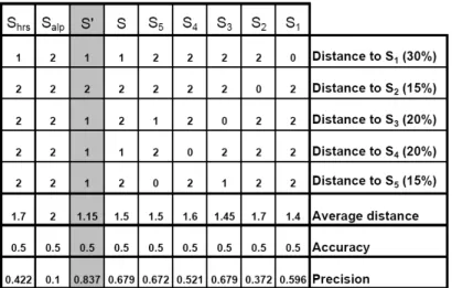
Fig. 11.The number of biases when adapting different models
The matrix in Fig. 11 shows how many biases would exist if we set different process models as the new reference process model. For example, if we set S1 as the new reference model, we therefore can find biases existing in S2, S3, S4, and S5, and the distances between S1 to them all equal 2. When given the percentage of each variants as the weight, we can compute the average weighted distances betweenS1 and the five variants in the repository. The number is 1.4 as shown in Fig. 11. We can interpret it as follows: if setting S1 as the new reference model, we need to perform on average 1.4 changes to the reference process model in order to configure it to the process variants in the repository.
Similarly, we can compute the average distance when setting other models as the
reference model. The result shows thatS0 (c.f. Fig. 8), the process model mined out using the method we suggested, has the shortest average weighted distance to the variants. It means, settingS0 as the new reference process model would require the least amount effort for process configuration, i.e. we only need to perform on average 1.15 changes to configure S0 into the five process variants.
Please note that the process models Salp andShrs, which are produced by the process mining algorithms based on traces, are in fact the two of the worst ones concerning the number of biases in the system. This result also corresponds the analysis we shown in Section 3.
When comparing the accuracy and precision of each process models, the mined out process model, S0, is still the best one. Although the accuracy for each process model all equals to 0.5, S0 has the highest precision value, 0.837 as shown in Fig. 11, which shows that S0 fits closer to the process variants in the repository. In addition, according to the results in Fig. 11, we can generally claim that the higher the precision value is, the shorter the average distance it has compared to the process variants. However, it does not always hold, for instance,S3has both higher precision value and average weighted distance when compared toS1. Such occasional in-consistency is not surprising due to theN P nature of the distance measure.
Clearly, it is not possible to enumerate all process models available, since it can be infinite. Therefore we can not prove that the process model we mined out are the best one. It is also possible that there exists better ones since the algorithm only search for local optimal as most data mining algorithms do [14].
However, as identified In Fig. 11, the mined out process model is at least better than all the process models currently known and the process models which can be produced by process mining algorithms based on executions. Keeping our search at local optimal will also make our approach applicable to really case, since we therefore can limit the complexity at polynomial level.
7 Mining Process Variants with Different Activity Set
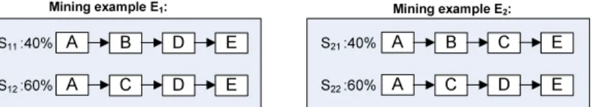
In Section 5 we introduced our method to mine process variants with the same set of activities. In practise, it is often the case that different process variant has different set of activities. In this section, we will discuss the technique to handle this situation. We explain our method by using two examplesE1 andE2
as described in Fig. 12. We will show how we mine the process variants with different activity set and why we do it in the proposed way.
In Fig. 12, we shows two examples. In example E1, there are two process variantsS11 and S12 which corresponding to 40% and 60% of the instances in the system. There are two activities: activityBand activityCthat do not appear together in any of the instances. Therefore, there is no process variant which can specify the execution order between activity BandC. However, when compared to the rest of activities, the execution order of B in S11 are the same as the execution order of Cin S12.