Discovering Reference Process Models by Mining Process Variants
Chen Li University of Twente
The Netherlands lic@cs.utwente.nl
Manfred Reichert University of Ulm
Germany
manfred.reichert@uni-ulm.de
Andreas Wombacher University of Twente
The Netherlands a.wombacher@utwente.nl
Abstract
Recently, a new generation of adaptive Process-Aware Information Systems (PAIS) has emerged, which allows for dynamic process and service changes (e.g., to insert, delete, and move activities and service executions in a running pro- cess). This, in turn, has led to a large number of process variants derived from the same model, but differing in struc- ture due to the applied changes. Generally, such process variants are expensive to configure and difficult to maintain.
This paper provides a sophisticated approach which fosters learning from past process changes and allows for mining process variants. As a result we obtain a generic process model for which the average distance between this model and the respective process variants becomes minimal. By adopting this generic model in the PAIS, need for future process configuration and adaptation decreases. We have validated the proposed mining method and implemented it in a powerful proof-of-concept prototype.
1 Introduction
In today’s dynamic business world, success of an enter- prise increasingly depends on its ability to react to changes in its environment in a quick, flexible and cost-effective way. Along this trend a variety of process and service sup- port paradigms as well as corresponding specification lan- guages (e.g., WS-BPEL, WS-CDL) have emerged. In ad- dition, different approaches for flexible and adaptive pro- cesses exist [9, 11]. Generally, process and service adap- tations are not only needed for configuration purposes at buildtime, but also become necessary during runtime to deal with exceptional situations and changing needs; i.e., for sin- gle instances of composite services and processes respec- tively, it must be possible to dynamically adapt their struc- ture (e.g. to insert, delete or move activities during runtime).
In response to this need adaptive process management
0Supported by the Netherlands Organization for Scientific Research (NWO) under contract number 612.066.512
technology has emerged [17]. It allows to adapt and config- ure process models at different levels. This, in turn, results in large collections of process model variants (process vari- ants for short), which are created from the same process model, but slightly differ from each other in their structure.
Generally, a large number of process variants may exist in a Process-Aware Information System (PAIS) [8]. As ex- ample take an automotive supply chain where a supplier of car parts requires different process variants per car manu- facturer and potentially per car model. This results in a high number of process variants, which is comparable to the number of customers of the supplier. To support the differ- ent choreographies the supplier requires the same number of orchestrations, i.e., process variants which have to be mod- eled and maintained. This number further increases when considering concrete cases as well. Here ad-hoc deviations from the standard processes occur frequently at process in- stance level, resulting in a multitude of process variants.
In most approaches which allow to adapt and config- ure process models, the resulting process variants have to be maintained separately. Then even simple changes (e.g.
due to new laws) might require manual re-editing of a large number of process variants. Over time this leads to de- generation and divergence of the respective process models, which aggravates maintenance significantly [4].
Though considerable efforts have been made to ease pro- cess configuration and customization [9, 11, 4], we do not yet utilize the knowledge resulting from these process adap- tations. Fig. 1 describes the goal of this paper. We aim at learning from past process changes by ”merging” process variants into one generic process model, which ”covers”
these variants best. By adopting this generic model asref- erence process modelwithin the PAIS, cost of change and need for future process adaptations will decrease.
Based on the two assumptions that (1) process models are well-formed (i.e., block-structured like in BPEL) and (2) all activities in a process model have unique labels, this paper deals with the following fundamental research ques- tion: Given a set of process variants, how to derive a refer- ence process model out of them, such that the average dis-
…
Reference process model S customization & adaptation
Process variant S1 Process variant S2 Process variant Sn
mining & learning
Reference process model S’ as learned from process variants Feedback
evaluation
Figure 1. Mining a new reference model with less expected changes
tance between the reference model and the process variants becomes minimal?
The distance between the reference process model and a process variant is measured by the number of high-level change operations (e.g., to insert, delete or move activities [9]) needed to transform the reference model into the vari- ant. Furthermore, change distance directly represents the ef- forts needed for process adaptation and customization. Ob- viously, the challenge is to find the ”best” reference model, i.e., the one with minimal average distance to the variants.
Sec. 2 gives background information needed for under- standing this paper. In Sec. 3 we introduce a method to represent process models in a way such that they can be mined effectively. Sec. 4 presents our algorithm for min- ing process variants. We validate it in Sec. 5 and sketch a proof-of-concept prototype in Sec. 6. Sec. 7 discusses related work. We conclude with a summary in Sec. 8.
2 Backgrounds
We first introduce basic notions needed in the following:
Process Model: LetPdenote the set of all sound process models. A particularprocess modelS = (N, E, . . .)∈ P is defined as well-structured Activity Net [9]. N consti- tutes the set of process activities andE the set of control edges (i.e., precedence relations) linking them. To limit the scope, we assume Activity Nets to be block-structured (like in BPEL). An example is depicted in Fig. 2.
Process change: We assume that a process change is ac- complished by applying a sequence of change operations to a given process modelSover time [9]. Such change opera- tions modify the initial process model by altering the set of activities and their order relations. Thus, each application of a change operation results in a new process model. We defineprocess changeandprocess variantsas follows:
Definition 1 (Process Change and Process Variant) Let P denote the set of possible process models andC be the set of possible process changes. Let S, S ∈ P be two process models, let Δ ∈ C be a process change, and let
σ = Δ1,Δ2, . . .Δn ∈ C∗ be a sequence of process changes performed on initial modelS. Then:
• S[ΔSiffΔis applicable toS andSis the (sound) process model resulting from the application ofΔ to S. We also denoteSasvariantofS.
• S[σS iff∃S1, S2, . . . Sn+1∈ P withS =S1,S = Sn+1, andSi[ΔiSi+1fori∈ {1, . . . n}.
Examples of high-level change operations includeinsert activity,delete activity, andmove activityas implemented in the ADEPT change framework [9]. While insert and delete modify the set of activities in the process model, movechanges activity positions and thus the structure of the process model. For example, operationmove(S,A,B,C) moves activity Afrom its current position within process model S to the position after activityBand before activ- ity C. Operation delete(S,A), in turn, deletes activity A from process model S. Issues concerning the correct use of these operations, their generalizations, and formal pre- /post-conditions are described in [9]. Though the depicted change operations are discussed in relation to ADEPT, they are generic in the sense that they can be easily applied in connection with other process meta models as well [17]. For example, a process change as realized in the ADEPT frame- work can be mapped to the concept of life-cycle inheritance known from Petri Nets [14]. We refer to ADEPT since it covers by far most high-level change patterns and change support features when compared to other approaches [17].
Definition 2 (Bias and Distance) Let S, S ∈ P be two process models. Then: Distanced(S,S)betweenS andS corresponds to the minimal number of high-level change operations needed to transform S intoS; i.e., d(S,S) :=
min{|σ| | σ ∈ C∗ ∧S[σS}. Furthermore, a sequence of change operationsσ withS[σS and |σ| = d(S,S) is denoted asbiasbetweenSandS.
The distance between process models S and S is the minimal number of high-level change operations needed for transforming S into S. The corresponding sequence of change operations is denoted asbiasbetweenSandS.1 Usually, the distance between two process models measures the complexity for model transformation or configuration.
As example take Fig. 3. Here, distance between modelS and variantS1 isone, since we only need to perform one change operationmove(S,E,A,D)to transformSintoS1
[7]. In general, determining the bias and distance between two process models has complexity atN Plevel [7].
Here, we use high-level change operations rather than change primitives (i.e., elementary changes like adding/removing nodes and edges) to measure the distance
1Generally, it is possible to have more than one minimal set of change operations to realize the transformation fromSintoS, i.e., given process modelsSandStheir bias needs not to be unique. A detailed discussion of this issue can be found in [14, 7].
between process models. This allows to guarantee sound- ness of process models and also provides a more meaning- ful measure for distance [7].
Trace: A trace t on process model S = (N, E, . . .) denotes a valid and complete execution sequence t ≡<
a1, a2, . . . , ak >of activitiesai∈NonSaccording to the control flow set out byS. All traces process modelS can produce are summarized in trace setTS.t(a≺b)is denoted as precedence relation between activitiesa andbin trace t≡< a1, a2, . . . , ak>iff∃i < j:ai=a∧aj=b. Here, we only consider traces composing ’real’ activities, but no events related to silent ones (i.e., activity nodes which con- tain no operation and exist only for control flow purpose [7]). Finally, we will consider two process models being the same if they aretrace equivalent, i.e.,S≡SiffTS ≡ TS.
3 Represent Process Models as Order Matrices
Theoretical backgrounds of high-level change operations have been extensively discussed in ADEPT [9]. One key feature of our ADEPT change framework is to maintain the structure of the unchanged parts of a process model [9]. For example, if we delete an activity this will neither influence the successors nor predecessors of this activity, and therefore also not their order relations. To incorpo- rate this feature in our approach, rather than only looking at direct predecessor-successor relationships between two ac- tivities (i.e., control edges), we consider the transitive con- trol dependencies between all activity pairs; i.e., for process model S = (N, E, . . .) ∈ P, for every pair of activities ai, aj∈N,ai =ajtheir order relations compared to each other are examined. Logically, we determine order relations by considering all traces the respective process model can produce (cf. Sec. 2). Results are aggregated in a matrix A|N|×|N|, which considers four types of control relations (cf. Def. 3):
Definition 3 (Order matrix) LetS = (N, E, . . .)∈ Pbe a process model withN ={a1, a2, . . . , an}. Let furtherTS
denote the set of all traces producible onS. Then: Matrix A|N|×|N|is calledorder matrixofSwithAijrepresenting the order relation between activitiesai,aj∈N,i =jiff:
• Aij = ’1’ iff (∀t∈ TSwithai, aj∈t⇒t(ai≺aj)) If for all traces containing activitiesaiandaj,ai al- ways appearsBEFOREaj, we denoteAij as ’1’, i.e., aialways precedes ofaj in the flow of control.
• Aij = ’0’ iff (∀t∈ TSwithai, aj∈t⇒t(aj≺ai)) If for all traces containing activitiesaiandaj,ai al- ways appearsAFTERaj, we denoteAijas a ’0’, i.e., aialways succeeds ofajin the flow of control.
• Aij= ’*’ iff (∃t1∈ TS, withai, aj∈t1∧t1(ai≺aj))
∧(∃t2∈ TS, withai, aj∈t2∧t2(aj≺ai))
If there exists at least one trace in whichai appears beforeajand another trace in whichaiappears after
aj, we denoteAijas ’*’, i.e.,aiandajare contained in different parallel branches.
• Aij = ’-’ iff (¬∃t∈ TS:ai∈t∧aj ∈t)
If there is no trace containing both activityaiandaj, we denoteAij as ’-’, i.e.,ai andaj are contained in different branches of a conditional branching.
A
C B
E
F G D
Process model S Order matrix of S
Activities in a same block
AND-Split AND-Join
XOR-Split XOR-Join
‘0’ : successor
‘1’ : predecessor
‘*’ : AND-block
‘-’ : XOR-block
Figure 2. Process model and its order matrix Fig. 2 shows an example. Besides control edges, which express direct predecessor-successor relationships, modelS also contains four kinds of control connectors: AND-Split and AND-Join (corresponding toflowin BPEL), XOR-Split and XOR-join (corresponding toswitchorpickin BPEL).
The order matrix can represent all these relationship. For example, activitiesAandBnever appear in the same trace since they are contained in different branches of an XOR block. Therefore, we assign ’-’ to matrix element AAB. Similarly, we obtain the relation for each pair of activities.
The main diagonal of the matrix is empty since we do not compare an activity with itself.
Under certain conditions, an order matrix uniquely rep- resents the process model it was created from. This is stated by Theorem 5. Before giving this theorem, we need to de- fine the notion ofsubstring of trace:
Definition 4 (Substring of trace) LetS ∈ P be a process model and lett, t ∈ TS be two traces onS. We denotet as sub-string of t iff [∀ai,aj ∈ t,t(ai ≺ aj) ⇒ai,aj
∈t∧t(ai≺aj)] and [∃ak∈N:ak ∈/ t∧ak∈t].
Theorem 5 Let S, S ∈ P be two process models with same activity set N = {a1, a2, . . . , an}. Let furtherTS, TS be the related trace sets andAn×n, An×n be the or- der matrices ofS andS. ThenS = S ⇔ A = A, if [¬∃t1, t1 ∈ TS: t1 is a substring of t1] and [¬∃t2, t2 ∈ TS:t2is a substring oft2].
We give a proof of Theorem 5 in [7]. According to The- orem 5, there will be a one-to-one mapping between a pro- cess modelS and its order matrixA, if the substring con- straint is met. (Note that the substring constraint can be easily checked and handled [7]); i.e., if the conditions of Theorem 5 are met, the order matrix will uniquely represent the process model. Analyzing its order matrix (cf. Def. 3) will then be sufficient in order to analyze the process model.
Using the order matrix, we can easily identify activities belonging to the same block. In particular, such activities have the same order relations with respect to activities from outside this block. As example, take the order matrix de- picted in Fig. 2. If we ignore the internal relation between
activities A and B, the order relations between A and all other activities are the same as forB(as marked up in Fig.
2, where the first two rows are identical when ignoring the order relation betweenAandB). Based on the order matrix, we can determine a process block containingAandB; fur- ther these activities are contained in different branches of an XOR-block (as indicated byAAB = ’-’). Our algorithm for mining process variants (cf. Sec. 4) utilizes the sketched representation form and block concept.
4 Discovering Reference Process Models
We present a sophisticated algorithm for mining a col- lection of process variants. Our goal is to derive a new ref- erence model which is easier configurable than the current one. Since we restrict ourselves to block-structured pro- cess models, we can build the new reference model by en- larging blocks, i.e., we first identify two activities that can form a block, then we merge this block with other activ- ities and blocks respectively to form a larger block. This procedure continues until all activities and blocks respec- tively are merged into one single block. This block and its internal structure then represent the new reference process model, we are looking for.
Our approach for mining process variants is as follows:
1. For all process variants calculate their order matrices and aggregate them to one high-dimensional matrix representing the whole variant collection (Sec. 4.1).
2. Based on this high-dimensional matrix, determine ac- tivities to be clustered in a block (Sec. 4.2).
3. Determine the order relation the clustered activities shall have within this block. (Sec. 4.3).
4. After building a new block in Steps 2 and 3, re- flect the clustering of activities by adjusting the high- dimensional matrix accordingly (Sec. 4.4).
5. Repeat Steps 2, 3 and 4 until all activities are clus- tered together, i.e., until the new process model is con- structed by enlargement of blocks.
These five steps are explained in the following. An il- lustrative example is given in Fig. 3. Reference model S has been configured into five process variants Si ∈ P (i = 1,2, . . .5), which are weighted based on the number of process instances created from them. In our example, 30% of all process instances were executed according to variant S1, while 15% of the instances did run onS2. If we only know process variants, but have no runtime infor- mation about related instance executions, we will assume the variants to be equally weighted; i.e., every process vari- ant has weight1/n, wherencorresponds to the number of variants in the system.
We can easily compute the distances (cf. Def. 2) be- tween reference model and process variants. For example,
when comparingSwithS1we obtain distanceone(cf. Fig.
3). Note that we only need to perform one change oper- ation (i.e., move(S,E,A,D); cf. Def. 1) to transformS intoS1. Or when comparingSwithS2, needed change op- erations are move(S,D,B,C)andmove(S,E,B,C), and distance between S and S2 is two. Based on the weight of each variant, we can compute average weighted distance between reference model S and its variants; e.g., the dis- tances betweenSandSiare 1(i=1), 2(i=2), 2(i=3), 1(i=4), and 2(i=5); and the weights are 30%, 15%, 20%, 20%, and 15% (cf. Fig. 3). Thus average weighted distance equals 1×0.3+2×0.15+2×0.2+1×0.2+2×0.15 = 1.5. This means we need to perform on average 1.5 change operations to configure the reference model to a process variant or re- lated instance respectively. Generally, the average weighted distance between a reference model and the process variants represents how ”close” they are. The goal of our mining al- gorithm is to discover a reference model for a collection of (weighted) process variants with minimal average weighted distance to these process variants. In the following, we as- sume that each process variant has the same activity set (for a relaxation of this constraint see [6]).
Process configuration
S1: 30%
S2: 15%
S3: 20%
S4: 20%
S5: 15%
B C
E
A D
D
A C B E
A D
E
B C
B E
A
C
D
A E
B
C
D
Weight of process variant, based on number of executions
Distance (S, S1) = 1
Distance (S, S2) = 2
Distance (S, S3) = 2
Distance (S, S4) = 1
Distance (S, S5) = 2
Average weighted distance = 1.5 change / instance
A B C D E
S: reference process model
AND-Split AND-Join XOR-Split XOR-Join
Figure 3. Illustrative example 4.1 Aggregated Order Matrix
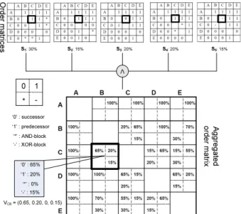
For the given collection of process variants, we first com- pute the order matrix (cf. Def. 3) for each process variant.
In our case, we need to determine five order matrices (cf.
Fig. 4). Afterwards, we analyze the order relation for each pair of activities considering all order matrices derived be- fore. As the order relation between two activities might be not the same in all order matrices, this analysis does not re- sult in a fixed relationship, but provides a distribution for the four types of order relations (cf. Def. 3). Regarding our example, activityCis in 65% of all cases a successor of activityB(as inS1,S2,S4), in 20% of all cases a pre- decessor ofB(as inS3), and in 15% of the casesBandC
are contained in different branches of an XOR block (as in S5) (cf. Fig. 4). Therefore, we can define the order re- lation between two activitiesa andb as a 4-dimensional vector Vab = (vab0 , vab1 , v∗ab, vab−): each field then corre- sponds to the frequency of the respective relation type (’0’,
’1’, ’*’ or ’-’) as specified in Def. 3. Take our example from Fig. 4; here v1CBcorresponds to the frequency of all cases with activitiesBandChaving order relationship ’1’, i.e., whereCis predecessor ofB. In our example, we obtain VCB = (0.65,0.2,0,0.15).
We define anaggregated order matrixas follows:
Definition 6 (Aggregated Order Matrix) Let Si ∈ P, i = 1,2, . . . , n be a collection of process variants with same activity set N. Let further Ai be the order ma- trix ofSi, and let wi represent the number of process in- stances being executed based onSi. TheAggregated Order Matrixof all process variants is defined as 2-dimensional matrix Vm×m with m = |N| and each matrix element vjk= (vjk0 , vjk1 , v∗jk, v−jk)being a 4-dimensional vector. For τ ∈ {0,1,∗,−}, elementvjkτ expresses to what percentage, activitiesajandakhave order relationτwithin the collec- tion of process variantsSi. Formally: ∀aj, ak ∈ N, aj = ak:vjkτ =(n
i=1,Aijk=τwi)/(n
i=1wi).
The aggregated order matrixV for the process variants from Fig. 3 is shown in Fig. 4.
In an aggregated order matrix, main diagonal is always empty since we do not specify the order relation of an ac- tivity with itself. For all other elements, a non-filled value in a certain dimension means it corresponds to zero.
In Section 3 we have shown that we can use an order matrix to determine blocks in a process model: i.e., two ac- tivities can be clustered into a block if they have same order relation with respect to other activities. As we will show,
0 1
* -
‘0’ : successor
‘1’ : predecessor
‘*’ : AND-block
‘-’ : XOR-block
S1: 30% S2: 15% S3: 20% S4: 20% S5: 15%
V
VCB= (0.65, 0.20, 0, 0.15)
‘0’ : 65%
‘1’ : 20%
‘*’ : 0%
‘-’ : 15%
Ordermatrices Aggregatedorder matrix
Figure 4. Aggregated order matrixV
similar idea can be applied when analyzing an aggregated order matrix. Our goal is to derive an optimal reference process model for the given variants from this representa- tion form.
4.2 Determine Activities to Be Clustered This subsection describes how to derive blocks of our reference model based on an aggregated order matrix.
There are two issues we have to consider. First, we have to decide which activities shall be blocked. Second, we must choose an order relation for them. This subsection deals with the first issue, the second one is addressed in Sec. 4.3.
In an order matrix, two activities can be clustered in a block if they have same order relations with respect to the other activities (cf. Sec. 3). We can apply similar idea when analyzing an aggregated order matrix. However, in an aggregated order matrix, the relationship between two ac- tivities is expressed as 4-dimensional vector showing the distributions of the order relations over all process vari- ants. When determining the activities that can be clustered in a block, it would be too restrictive to require precise matching as in the case of an order matrix. For this rea- son, we first introduce function f(α, β) which expresses the closeness between two vectorsα= (x1, x2, ..., xn)and β = (y1, y2, ..., yn):
f(α, β) = α·β
|α| × |β| =
n
i=1xiyi
n
i=1x2i ×n
i=1yi2 f(α, β) ∈ [0,1]computes the cosine value of the an- gleθbetween the two vectorsαandβ in Euclid space. If f(α, β) = 1holds, αand β will exactly match in their directions; f(α, β) = 0 means, they do not match at all.
When comparing closeness between vBE and vCE, for in- stance, we obtainf(vBE, vCE) = 0.968. This high value im- plies that these two vectors are close to each other, though they are not the same.
Based on f(α, β) we introduce Separation. It indi- cates how well two activities of an aggregated order matrix are suited for being clustered in a block. More precisely, Separation(A,B)expresses how similar order relations of activitiesAandBare when compared to the rest of activ- ities. In our example from Fig. 3, Separation(A,B) is determined by the closeness (measured by the cosine value) off(vAC, vBC),f(vAD, vBD)andf(vAE, vBE). Generally, we define cluster separation as follows:
Separation(a, b) =
x∈N\{a,b}f2(vax, vbx)
|N| −2
Ncorresponds to the set of activities. Like most cluster- ing algorithms [13], we square the cosine value to empha- size the differences between the two compared vectors. Fi- nally, by dividing this expression by|N| −2, we normalize
its value to a range between [0, 1]. Regarding our example from Fig. 3, we obtainSeparation(A,B) = 0.905.
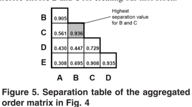
We determine the pair of activities mostly suited to form a block by measuring how much each pair of activities is separated from the others. We accomplish this by comput- ing the separation value for each activity pair. The higher this value is, the more suited the two activities are for be- ing clustered. For our example from Fig. 3, the separation values are shown in Fig. 5. We denote this table assepa- ration table. It becomes clear that activitiesBandChave the highest separation value 0.936 (marked up in grey). We therefore chooseBandCfor creating our first block.
Highest separation value for B and C
Figure 5. Separation table of the aggregated order matrix in Fig. 4
4.3 Determine Internal Order Relations After having decided that activitiesBandCshall be first clustered in a block, we have to determine the order rela- tion these two activities shall have. In addition, we measure how good such choice is. For this purpose, we introduce Cohesion, which indicates how significant particular order relations between two activities of the same cluster are.
In our aggregated order matrix, the relationship between activities B and C is depicted as a 4-dimensional vector vBC = (0.2,0.65,0,0.15). It shows the distribution values of the four types of order relations in a 4-dimensional space.
Obviously, when building a reference process model, only one of the four order relations can be chosen. Therefore, we want to choose that type of order relation which is most sig- nificant when compared to the others. Regarding our exam- ple, the significance of each order relation can be evaluated by the closenessvBCand the four axes in the 4-dimensional space have. These four axes can be represented by four benchmarking vectors: v0 = (1,0,0,0),v1 = (0,1,0,0), v∗ = (0,0,1,0), andv− = (0,0,0,1). Therefore, we can compute the significance of each order relation using for- mulaf(α, β)(cf. Sec. 4.2), whereα=vBCandβis one of the four benchmarking vectors. Regarding our example, the closest axis tovBCisv1(f(vBC, v1)= 0.933). Therefore, we decide thatBshall precedeCwithin the derived block (cf.
Def. 2).
We can use cohesion to evaluate how good our choice is:
Cohesion(a, b) =
2×max{f(vab, v0), f(vab, v1), f(vab, v∗), f(vab, v−)}−1
The measure has value range [0,1].Cohesion(a, b)will equal one if there is a dominant order relation, i.e., vab
is on one of the four axes. Cohesion(a, b) will equal zero if vab is (0.25,0.25,0.25,0.25), i.e., no order rela- tion is more significant than others. Regarding our example, Cohesion(B,C)equals 0.867. This indicates high signifi- cance for settingBas predecessor ofC.
4.4 Recompute the Aggregated Order Matrix
We have discovered the first block of our reference pro- cess model, which contains BandC. We have further de- cided that Bshall precede C, and that the significance of this order relation is 0.867. We now have to decide on the relationship between this newly created block and the other activities.
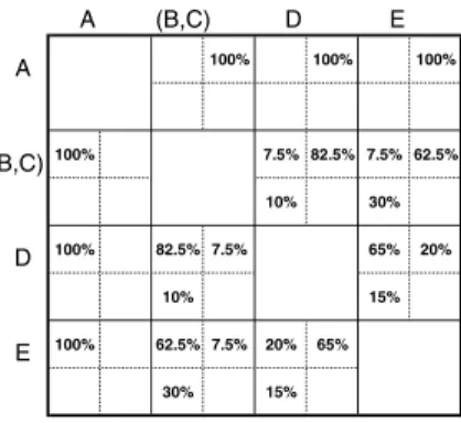
Regarding the process variants from Fig. 3,BandCdo not always constitute an elementary block (i.e., a block only containingBandC). To be more precise,BandCrepresent an elementary block in S1, S3 andS5, but not inS2 and S4. Nevertheless,BandCare most suited to form a block based on our analysis of the aggregated order matrix. This requires adaptation of the original aggregated order matrix in order to represent the situation in whichBandCare clus- tered in a block.2 We accomplish this adaptation by com- puting the means of the order relations between{B,C}and the remaining activities. For example, asvBD = (0,1,0,0) andvCD = (0.15,0.65,0.2,0) hold, the order relation be- tween the newly created block (B,C) and activityDwill be (vBD+vCD)/2 = (0.075,0.825,0.1,0). Such computation is applied to all remaining activities outside this block.
Generally, after clustering activities a and b, the new aggregated order matrixVcan be calculated as follows:
1. ∀x∈N\ {a, b}:
v(a,b)x = (vax+vbx)/2 vx(a,b) = (vxa+vxb)/2 2. ∀x, y∈N\ {a, b}:vxy =vxy
The aggregated order matrixVwe obtain after cluster- ingBandCis shown in Fig. 6. SinceBandCare replaced by a block containing them, the matrix resulting after the re- computation is one dimension smaller thanV. Afterwards, we treat this block like a single activity.
4.5 Mining Result and Evaluation
After obtaining a newly aggregated order matrix, we re- peat the three steps as described in Sec. 4.2, 4.3 and 4.4;
i.e., first identify the activities (and blocks respectively) to be clustered, then determine their order relation within the block, and finally re-compute the aggregated order matrix considering the newly determined block. In every iteration,
2Our approach is different to traditional clustering algorithms [13], in which only distances are re-computed, but not the original dataset. We give a discussion why we need to change the original dataset in [6].
A (B,C) D E
A 100% 100% 100%
(B,C)100% 7.5% 82.5% 7.5% 62.5%
10% 30%
D 100% 82.5% 7.5% 65% 20%
10% 15%
E 100% 62.5% 7.5% 20% 65%
30% 15%
Figure 6. New aggregated order matrixVaf- ter clusteringBandC
we merge two activities (and blocks respectively) into a big- ger block. This iterative clustering continues until all activ- ities (and blocks respectively) are clustered; then we have constructed the new reference model. Obviously, the num- ber of required iterations equals the number of activities mi- nus one. The final result after all iterations is shown in Fig.
7.
Fig. 7 shows the process modelS we have discovered through mining the variants from Fig. 3. It also shows how such result is constructed after every iteration (shown as a number at the right-bottom corner of each block). In itera- tion 1,BandCare clustered to form a block; in the next it- eration, such block is enlarged by clustering activityEwith it. Finally, after the fourth iteration, all activities have been clustered together into a single block, i.e., we have obtained our new reference model. Fig. 7 also shows cohesion val- ues, which reflect the significance of the order relations we haven chosen in the different iteration.
5 Validation
The complexity of the mining algorithm described in Sec. 4 corresponds toO(n3). Like most clustering algo- rithms in data mining [13], this algorithm is trying to solve a complex combinatorial optimization problem in polyno- mial time. This leads to the benefit that it can solve a prob- lem with large scale, but has the disadvantage that it only searches for a local, but not global optimum. Therefore, it is not possible to prove that the algorithm really does what we want, i.e., to reduce biases in the system by improving the reference process model.
However, we can compare the process model discovered with our mining method with some other models. This com- parison is based on how many high-level change operations
0.867
B C 0.792 E 0.939 D
A 1.0
1 2
3 4
Figure 7. The resulting process modelS
are required to configure the respective process variants out of the reference model (cf. Def. 2). For this purpose, for each candidate model Scan, we assume that it is con- sidered as the new reference model and then calculate the average weighted distance betweenScan and the five vari- antsS1−S5; e.g., in Fig 3 the average weighted distance betweenS and the five variants is 1.5, which reflects how close the current reference model is to the process variants.
Using same method, we can compute the average weighted distance between candidate reference modelScanand vari- antsS1−S5.
There are two groups of process models that are candi- dates for becoming the new reference process model. The first group contains all models we already know. Clearly, reference modelSand the five variantsS1, S2, S3, S4and S5(cf. Fig. 3) belong to this group. Comparing these exist- ing models with the one we obtained through process vari- ant mining, for example, already shows that it is not suf- ficient to simply set the reference model to the most fre- quently used process variant (S1in our example).
The second group includes the process models we can discover through mining. Clearly, process model S (cf.
Fig. 7), as obtained with our algorithm for process vari- ant mining, belongs to this group. So far there has been no algorithm directly supporting the mining of process vari- ants. Therefore, we apply traditional techniques from the field of process mining[15], and compare them with our approach. The goal of process mining techniques is to dis- cover process models from execution log. An execution log typically documents the start and/or end of each activity in a PAIS, and therefore reflects PAIS’s behavior. In our case, we assume that the behavior of all process variants is fully covered by an execution log, i.e., we enumerate all traces producible by each process variant from Fig. 3 (cf. Fig.
8). We then use them as input for different process mining techniques. We consider Alpha algorithm [16], Alpha++
algorithm [19], Heuristics Mining [18], and Genetic Min- ing [2], which are some of the most well-known algorithms for discovering process models from execution logs. The discovered process models are shown in Fig. 8. Both Al- pha and Alpha++ algorithm result in model Salp, whereas Heuristics mining provides modelShrs. We do no consider the model discovered by genetic mining, since it is too dif- ferent; i.e., genetic mining resulted in a complex model with six silent activities (and the distances to each process variant is higher thanthree).
Salp: Alpha, Alpha ++, algorithm A
E
C
B D A D
E
C B
Shrs:Heuristics mining S1:30% : {AEBCD, ABECD, ABCED}
S2:15% : {ABDEC, ABEDC}
S3:20% : {ACBED}
S4:20% : {ABCDE, ABDCE}
S5:15% : {ABED, ACED}
Process mining Trace sets
Figure 8. The candidate process models
We now compute the distances between each candidate modelScanfrom the two groups and the five process vari- antsS1 −S5. Further, we compute the average weighted distance. Comparison results are depicted in Fig. 9. For ex- ample, if we consider process variantS1as reference model, the distance between this model and variantsS2, S3, S4, and S5will equal 2, and average weighted distance betweenS1
and the five process variants will be 1.4 (cf. columnS1in Fig. 9). This means that when choosingS1as new reference model we would need to perform on average 1.4 changes to configure the process variants out ofS1. Similarly, we can compute distances for the other candidate models. Alto- gether, results from Fig. 9 show thatS (cf. Fig. 7) –the process model resulting from the approach we suggested –has the shortest average weighted distance to the given process variants. This means, settingS as new reference process model would require lowest efforts for configuring the variants. More precisely, we only need to perform on average 1.15 changes to configure a process variant out of S. Note that process models Salp andShrs, we discov- ered by applying conventional process mining algorithms (based on traces), show the largest average distance to the five variants. We obtained similar results when mining other collections of process variants.
Comparison results do not imply that process variant mining is better than process mining. Each of them has different inputs and goals. Compared to process mining, which tries to discover the underlying process model by learning from the behavior of a system, process variant min- ing focuses on discovering a reference process model which can be easily configured to the different process variants. If we apply the process mining evaluation criteria to measure the result of process variant mining, the discovered process modelS (cf. Fig. 7) is also not good in terms of behav- ior, since the behavior ofS, which can be expressed by the trace set producible byS, is limited when compared to the trace sets the variants can produce. We give a detailed comparison in [6].
Obviously, it is not possible to enumerate all process models, since the number of process models can be infi- nite. However, as depicted In Fig. 9, the discovered process
Figure 9. The average weighted distance be- tween candidate models and the variants
model is at least better than the process models currently known and the process models which can be produced by process mining algorithms based on traces. Keeping our search at local optimum will also make our approach appli- cable to real cases, since we can limit complexity at poly- nomial level.
6 Proof-of-Concept Prototype
The described approach has been implemented and tested using Java. Figure 10 shows a screenshot of our pro- totype. We use ADEPT2 Process Template Editor [10] as the tool to create process variants. For each process model, the editor can generate an XML document with all infor- mation about the process model (like nodes, edges, blocks) being marked up. We store created variants in the variants repository folder”instances”(cf. Fig. 10) for mining.
The mining algorithm has been developed as stand-alone Java program, independent from the process editor. It can read the process variants and generate the result model ac- cording to the XML schema of the process editor. The re- sulting model is stored in the folder”miningResult”and can be visualized using the ADEPT2 editor.
7 Related Work
A variety of techniques for process mining has been suggested in literature [15, 18, 2, 16]. As illustrated in Sec. 5, traditional process mining is different from pro- cess variant mining due to its different goals and inputs.
[5] presents a method to mine configurable process mod- els based on event logs, but is still focusing on discover- ing process models from event logs rather than reducing efforts for process configuration. In addition, a few tech- niques have been proposed to learn from process variants by mining change primitives. [1] measures process model similarity based on change primitives and suggests mining techniques using this measure. However, this approach does not consider important features of our process meta model;
e.g., it is unable to deal with silent activities and it does
Figure 10. Screenshot of the prototype
also not differentiate AND- and XOR- branchings. Similar techniques for mining change primitives exist in the field of association rule mining [13] and maximal sub-graph min- ing [13] as known from graph theory [12]; here common edges between different nodes are discovered to construct a common sub-graph from a set of graphs. To mine high level change operations, [3] presents an approach based on process mining techniques, i.e., the input consists of a change log, and process mining algorithms are applied to discover the execution sequences of the changes (i.e., the change meta process). However, this approach simply con- siders each change as individual operation so that the result is more like a visualization of changes rather than mining them. [8] presents a method for retrieving process variants using a query model, but does not provide any mining sup- port. None of the discussed approaches aims at creating a reference process model, which allows for easy and opti- mized configuration for process variants in future.
8 Summary and Outlook
In this paper, we provide a sophisticated approach to mine block-structured process variants in order to discover a reference process model which can be easily configured to these variants. The proposed algorithm has polynomial complexity (O(n3)), which allows us to scale up when solv- ing real-world problems. Based on a quantitative analysis, we have shown that the reference model discovered with our approach is better (i.e., requires a low number of change op- erations for configuring the variants) than all process mod- els known in the system. It is also better than all models we can discover based on conventional process mining algo- rithms [15]. The validation result also implies that current process mining techniques cannot fulfill the goal of discov- ering a process model which is easily configurable. To our best knowledge, this paper has provided the first algorithm to support the mining of process variants with the goal of obtaining a reference model which is easily configurable.
Our approach looks promising, but there are still several questions left open. First we have to include more control structures (like loops or synchronization constraints for par- allel activities) as proposed in ADEPT [9] or BPEL. In ad- dition, we want to design search or heuristic algorithms to limit differences between original reference process model and the one we discover through variant mining. In this way, we can also limit the costs to update the old reference model to the new one.
References
[1] J. Bae, L. Liu, J. Caverlee, and W.B. Rouse. Process mining, discovery, and integration using distance measures. InICWS
’06, pages 479–488, Washington, DC, USA, 2006.
[2] A.K. Alves de Medeiros.Genetic Process Mining. PhD the- sis, Eindhoven University of Technology, NL, 2006.
[3] C.W. G¨unther, S. Rinderle, M. Reichert, and W.M.P. van der Aalst. Change mining in adaptive process management sys- tems. InCoopIS’06, pages 309–326, 2006.
[4] A. Hallerbach, T. Bauer, and M. Reichert. Managing process variants in the process lifecycle. InICEIS ’08, to appear, 2008.
[5] M.H. Jansen-Vullers, W.M.P. van der Aalst, and M. Rose- mann. Mining configurable enterprise information systems.
Data Knowl. Eng., 56(3):195–244, 2006.
[6] C. Li, M. Reichert, and A. Wombacher. Discovering pro- cess reference models from process variants using clustering techniques. Technical Report TR-CTIT-08-30, University of Twente, Enschede, March 2008.
[7] C. Li, M. Reichert, and A. Wombacher. On measuring pro- cess model similarity based on high-level change operations.
InER ’08, 2008.
[8] R. Lu and S.W. Sadiq. Managing process variants as an in- formation resource. InBPM’06, pages 426–431, 2006.
[9] M. Reichert and P. Dadam. ADEPT flex -supporting dynamic changes of workflows without losing control. Journal of In- telligent Info. Sys., 10(2):93–129, 1998.
[10] M. Reichert, S. Rinderle, U. Kreher, and P. Dadam. Adaptive process management with ADEPT2. InICDE ’05, pages 1113–1114. IEEE Computer Society, 2005.
[11] M. Rosemann and W.M.P. van der Aalst. A configurable reference modelling language.Inf. Syst., 32(1):1–23, 2007.
[12] K.H. Rosen. Discrete Mathematics and Its Application.
McGraw-Hill, 2003.
[13] P.N. Tan, M. Steinbach, and V. Kumar. Introduction to Data Mining. Addison-Wesley, 2005.
[14] W.M.P. van der Aalst and T. Basten. Inheritance of work- flows: an approach to tackling problems related to change.
Theor. Comput. Sci., 270(1-2):125–203, uary.
[15] W.M.P. van der Aalst, B.F. van Dongen, J. Herbst, L. Maruster, G. Schimm, and A.J.M.M. Weijters. Workflow mining: a survey of issues and approaches. Data Knowl.
Eng., 47(2):237–267, 2003.
[16] W.M.P van der Aalst, T. Weijters, and L. Maruster. Workflow mining: Discovering process models from event logs. IEEE Trans. on Knowl. and Data Eng., 16(9):1128–1142, 2004.
[17] B. Weber, S. Rinderle, and M. Reichert. Change patterns and change support features in process-aware information sys- tems. InCAiSE’07, pages 574–588, 2007.
[18] A.J.M.M. Weijters and W.M.P. van der Aalst. Rediscovering workflow models from event-based data using little thumb.
Integr. Comput.-Aided Eng., 10(2):151–162, 2003.
[19] L. Wen, J. Wang, and J. Sun. Detecting implicit dependen- cies between tasks from event logs. In APWeb’06, pages 591–603, 2006.