REFERENCE PROCESS MODELS OUT OF PROCESS VARIANTS
CHEN LI∗
Information Systems Group, University of Twente, The Netherlands, lic@cs.utwente.nl (contact author)
MANFRED REICHERT
Institute of Databases and Information Systems, University of Ulm, Germany, manfred.reichert@uni-ulm.de
ANDREAS WOMBACHER
Database Group, University of Twente, The Netherlands, a.wombacher@utwente.nl
During the last years a new generation of adaptive Process-Aware Information Systems (PAIS) has emerged, which enables dynamic process changes at runtime, while preserving PAIS robustness and consistency. Such adaptive PAIS allow authorized users to add new process activities, to delete existing activities, or to change pre-defined activity sequences during runtime. Both this runtime flexibility and process configurations at build-time, lead to a large number of process variants being derived from the same process model, but slightly differing in structure due to the applied changes. Generally, process variants are expensive to configure and difficult to maintain. This paper presents selected results from our MinAdept project. In particular, we provide a clustering algorithm that fosters learning from past process changes by mining a collection of process variants.
As mining result we obtain a process model for which average distance to the process variant models becomes minimal. By adopting this process model as reference model in the PAIS, need for future process configuration and adaptation decreases. We have validated our clustering algorithm by means of a case study as well as comprehensive simulations. Altogether, our vision is to enable full process lifecycle support in adaptive PAIS.
Keywords: process-aware information system; process change; process variants; process mining; process learning
1. Introduction
Economic success of an enterprise increasingly depends on its ability to react to changes in its environment (e.g., market changes or changes of legal regulations) in a quick, flexible and cost-effective way39,55,40,9. Along this trend a variety of process support paradigms as well as corresponding process specification and execution
* This work was done in the MinAdept project, which has been supported by the Netherlands Organization for Scientific Research (NWO) under contract number 612.066.512.
1
languages have emerged. Using WS-BPEL4, for example, a process can be composed out of existing services. At runtime, the execution of these services is orchestrated by theProcess-Aware Information System (PAIS) according to the defined process logic.
Generally, different scenarios for adaptive and configurable processes exist.70 Process adaptations are not only needed for configuration purposes at build-time
16,52, but also become necessary during runtime to deal with exceptional situations and changing needs41,69,24; i.e., for single process instances, it should be possible to dynamically adapt their structure, by inserting, deleting or moving process activities and process fragments respectively.
In response to this need adaptive process management technology has emerged.68,70 Basically, it enables adaptation and configuration of process models at different levels. This, in turn, results in large collections of process model vari- ants (process variants for short), which are created from the same process model, but slightly differ in structure from each other. Generally, a large number of pro- cess variants may exist in a PAIS 31,70,17. For example, according to a case study we performed in healthcare domain (details are discussed in Section 5), we have identified more than 90 process variants for one particular healthcare procedure.
In most approaches which allow to adapt and configure process models, the re- lated process variants have to be maintained separately.16Then even simple changes in process behavior (e.g. due to new laws) might require manual re-editing of a large number of related process variant models. Over time this leads to degeneration and divergence of these models, which aggravates PAIS maintenance significantly.
1.1. Problem Statement
Though considerable efforts have been made to ease process configuration and adap- tation16,41,52, we have not utilized the knowledge resulting from these process model changes yet.69 Fig. 1 describes the goal of our paper. We aim at learning from past process changes by ”merging” existing process variants into one generic process model, which ”covers” these variants best. By adopting this generic model asref- erence process model within the PAIS, cost of change and need for future process adaptations will decrease. Based on the two assumptions that (1) process models are well-formed (i.e., block-structured like in WS-BPEL) and (2) all activities in a process model have unique labelsa, we deal with the following fundamental research question:
Given a collection of process variants (i.e., process models), how to derive a reference process model out of them such that the average distance between the dis- covered reference model and the process variants becomes minimal?
The distance between reference process model and process variant is measured in
aThe block-structure constraint is discussed in detail in Section 2. Regarding the constraint in respect to unique labeling, we refer to11for an approach matching activities with different labels in different process variants.
…
reference process model S customization & adaptation
process variant S1 process variant S2 process variant Sn
mining & learning
reference process model S’ as learned from
process variants
feedback evaluation
Fig. 1. Mining a new reference model
terms of the number of high-level change operations (e.g., to insert, delete or move activities41) needed to transform the reference model into the model of the respec- tive variant. Furthermore,change distance directly represents the efforts needed for process adaptation and customization, and average distance between a reference model and a collection of process variants directly measures the configuration ef- forts for particular reference process model. Obviously, the challenge is to find the
”best” reference model, i.e., the one with minimal average distance to the known variants. Note that we only need a collection of process variants as input of our analysis. We do not need achange log, which specifically documents all change op- erations performed during the configuration of process variants15. In fact, even the original reference process model from which the variants are derived is not strictly required. In the following we present a clustering technique to deal with these chal- lenges.
1.2. Contribution
This paper significantly extends our work previously presented in25 and provides more technical details and validation results. For example, we relax the constraint of requiring a unique activity set, i.e., we provide an approach to cope with process variants having different activity sets. Further, we consider more workflow patterns (e.g., loop structures) when compared to previous work. For practical validation of our approach, a case study performed in the healthcare domain is added. Finally, this paper includes a detailed description of the implemented proof-of-concept pro- totype and conducts a simulation to examine scalability of our mining algorithm.
The clustering algorithm presented in this paper is completely different from the heuristics algorithm introduced in27: it has less rigid requirements regarding input data (e.g., an original reference process model is not required), and it can provide more detailed information on the discovered model (e.g., to what degree a certain part of the discovered model matches to the variants). Complexity of our clustering algorithm is polynomial, which is significantly lower than theN P-hard algorithm
presented in 27.
The remainder of this paper is organized as follows. Section 2 gives background information needed for understanding this paper. In Section 3 we describe funda- mental goals for mining process variants and discuss why we need an approach which differs from traditional process mining techniques. Section 4 introduces a method to represent process variant models in a way such that they can be mined effectively. We discuss a case study which we performed in healthcare filed in Sec- tion 5. Section 6 presents our basic clustering algorithm for mining process variants.
Section 7 extends it such that variants with different activity sets can be considered as well. We validate our algorithm in Section 8 by comparing its performance with existing process mining techniques. We formally specify our algorithm and sketch a proof-of-concept prototype in Section 9. Finally, Section 10 discusses related work and Section 11 concludes with a summary and outlook.
2. Backgrounds
We first introduce basic notions needed in the following:
Process Model: LetP denote the set of all sound (i.e., correct) process mod- els. We denote a process model as sound if there are no deadlocks or unreachable activities in the process model 41,62. In our context, a particular process model S= (N, E, . . .)∈ P is defined in terms of an Activity Net41:N constitutes the set of activities{a1, . . . , an}andE the set of control edges (i.e., precedence relations) linking them.bMore precisely, Activity Nets cover the following fundamental pro- cess patterns: Sequence, AND-split, AND-join, XOR-split, XOR-join, and Loop60.c These patterns constitute the core set of any workflow specification language (e.g., WS-BPEL 4 and BPMN 5) and cover most of the process models we can find in practice75,33. Furthermore, based on these patterns we are able to compose more complex ones if required (e.g., an OR-split can be mapped to AND- and XOR-splits
37). Finally, when restricting process modeling to these basic process patterns, we obtain models that are better understandable and less erroneous 36,34. A simple example of an Activity Net is depicted in Fig. 3a. For a detailed description of Activity Nets and relating correctness issues we refer to41.
Block Structuring: To limit the scope, we assume Activity Nets to be block- structured, i.e., sequences, branchings (based on the aforementioned split and join patterns), and loops are represented as blocks with well-definedstartandendnodes.
These blocks may be nested, but must not overlap; i.e., the nesting must be reg- ular 41,22. In a process modelS, a block may be a single activity, a self-contained part of S, or S itself. As example consider process model S from Fig. 3. Here {A}, {A,B}, {C,F}, and {A,B,C,D,E,F,G} describe possible blocks contained in
bAn Activity Net contains more elements than node setN and edge setE, which can be factored out in the context of this paper.
cThese patterns can be mapped to other languages as well. For example, in WS-BPEL (Business Process Execution Language), XOR-split / -join can be represented using ’If’ or ’Pick’. Further- more, AND-split / -join can be represented using ’Flow’, and Loops using ’RepeatUntil’4.
S. Note that we can represent a block B as activity set, since the block struc- ture itself becomes clear from process modelS. For example, block {A,B} corre- sponds to the parallel block with corresponding AND-split and AND-join nodes in S. The concept of block-structuring can be found in service composition lan- guages like WS-BPEL and XLANG4. Furthermore, adaptive process management systems like AristaFlow BPM Suite8and CAKE2 38 have emerged, which are ap- plied in a variety of application domains and whose process modeling language is block-structured as well. When compared with non-block-structured process mod- els, block-structured ones are easier understandable for users and have less chances of containing errors45,34,35,36,7. In a case study we conducted in another project, we investigated 214 process models expressed in different languages, like Event Process Chains, UML Activity Diagrams and WS-BPEL. More than 98% of these models were block-structured57. Finally, if a process model is not block-structured, in most practically relevant cases we can transform it into a block-structured one66,36,22. For all these reasons, we consider our approach for mining block-structured process variant models as being practically relevant.
Process change: A process change is accomplished by applying a sequence of high-level change operations to a given process modelS over time 41. Such oper- ations structurally modify the initial process model by altering its set of activities and/or their order relations. Thus, each application of a change operation results in a new process model. We defineprocess change andprocess variant as follows:
Definition 2.1. (Process Change and Process Variant) LetPdenote the set of possible process models andC be the set of possible process changes. LetS, S0∈ P be two process models, let∆∈ C be a process change, and letσ=h∆1,∆2, . . .∆ni ∈ C∗ be a sequence of changes performed on initial model S. Then:
• S[∆iS0iff∆is applicable toS andS0is the (sound) process model resulting from the application of ∆ toS.
• S[σiS0 iff ∃ S1, S2, . . . Sn+1 ∈ P with S =S1, S0 =Sn+1, andSi[∆iiSi+1
fori∈ {1, . . . n}. We also denoteS0 as process variantof S.
Examples of high-level change operations includeinsert activity,delete activity, andmove activity, but also more complex adaptations like move process fragment (i.e., a whole block) or surround process fragment with a loop structure as im- plemented in the ADEPT change framework41,8. While insert and delete enable modifying the set of activities in a process model,move changes activity positions and thus the structure of the process model. A formal semantics of these change patterns can be found in50. For example, change operationmove(S,A,B,C) moves activity A from its current position within process model S to the position after activity Band before activity C. Operationdelete(S,A), in turn, deletes activity A from process modelS. Finally, change operationinsert(S,A,B,C) adds activityAto the position after activityBand before activityC. Issues concerning the correct use of these change operations, their generalization, and formal pre-/post-conditions are
described in41. Though the depicted change operations are discussed in relation to our ADEPT change framework, they are generic in the sense that they can be easily applied in connection with other process meta models as well 50,68. For example, a process change as realized in the ADEPT framework can be mapped to the con- cept of life-cycle inheritance known from Petri Nets 58. We refer to ADEPT since it covers by far most high-level change patterns and change support features when compared to other adaptive PAIS68. Furthermore, with AristaFlow BPM Suite8, an industrial-strength version of the ADEPT technology emerged, which has been already applied in a variety of application domains.d
Based on the given set of change operations, we define the notions ofdistance andbias as follows:
Definition 2.2. (Bias and Distance) Let S, S0 ∈ P be two process models.
Then: Distance d(S,S0) between S and S0 corresponds to the minimal number of high-level change operations needed to transformS intoS0; i.e., we define
d(S,S0)= min{|σ|¯
¯σ∈ C∗∧S[σiS0} (1)
Furthermore, a sequence of change operations σ with S[σiS0 and |σ| = d(S,S0) is denoted as bias betweenS andS0.
The distance between process models S and S0 corresponds to the minimal number of high-level change operations needed for transforming S into S0. The corresponding sequence of change operations is denoted as bias BS,S0 between S andS0.e Usually, such distance measures the complexity for model transformation (i.e., model configuration). As example consider Example 1 in Fig. 2. Here, distance between reference process model S and process variant S1 is one, since we only need to perform change operation move(S,B,A,C) to transform S into S1 26. In general, determining bias and distance between two process models has complexity atN P-hardlevel26,59. We consider high-level change operations instead of change primitives (i.e., elementary changes like adding or removing nodes or edges in a process graph) to measure the distance between process models. Amongst others, this helps us to guarantee soundness of process models and further provides a more meaningful measure for distance26,68.
Finally, we define the notion of trace:
Definition 2.3. (Trace) Let S= (N, E, . . .)∈ P be a process model. We define t as a trace ofS iff:
• t ≡< a1, a2, . . . , ak > (with ai ∈N) constitutes a valid and complete exe- cution sequence of activities considering the control flow defined by S. We
dVisit www.aristaflow-forum.de for details.
eGenerally, it is possible to have more than one minimal set of change operations to transform SintoS0, i.e., given process modelsSandS0their bias does not need to be unique. A detailed discussion of this issue can be found in58,26.
define TS as the set of all traces that can be produced by process instances running on process modelS.
• t(a≺b)is denoted as precedence relationship between activities aandb in trace t≡< a1, a2, . . . , ak>iff∃i < j :ai=a∧aj =b.
We only consider traces composing ’real’ activities, but no events related to silent ones, i.e., nodes within a process model having no associated action and only existing for control flow purpose 26. Fig. 4 depicts some examples. At this stage, we consider two process models as being the same if they aretrace equivalent, i.e., S ≡S0 iff TS ≡ TS0. Like in most process mining approaches, the stronger notion of bi-similarity18is not considered in our context.
3. Mining Process Variants: Goals and Issues
This section discusses the major goal in respect to the mining of process variants, namely to derive ageneric process model from a collection of process variants. This shall be done in a way such that the existing variants (as well as future ones) can be efficiently configured out of the discovered generic model. We measure efforts for corresponding process configurations in terms of the number of high-level change operations needed to transform the discovered generic model into the respective model variant. The challenge is to find a generic model such that theaveragenumber of high-level change operations needed (i.e., theaverage distance) becomes minimal with respect to the given variant collection.
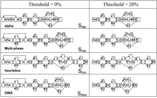
To make this more clear, we first compare process variant mining with traditional process mining.61 Process mining has been extensively studied in literature. Its key idea is to discover a process model by analyzing the execution behavior of (completed) process instances as captured in execution logs.61 Different mining techniques like alpha algorithm 63, heuristics mining 71 or genetic mining 10 have been proposed in this context. Obviously, input data for traditional process mining differs from the one for process variant mining. While traditional process mining operates on execution logs, mining of process variants is based on a collection of process model variants. Of course, such high-level consideration is insufficient to prove that existing mining techniques do not provide optimal results with respect to the aforementioned goal. In principle, existing process mining techniques 63,10 can be applied to our problem as well. For example, we could derive all traces producible by a given collection of process variants73and then apply existing mining algorithms to them. To make the difference between process and process variant mining more evident, in the following we consider behavioral similarity between two process models as well asstructural similaritybased on their bias (cf. Def. 2.2).
The behavior of a process modelS can be represented by the set of traces (i.e., TS) it can produce. Therefore, two process models can be compared based on the difference between their trace sets.63,73 By contrast, biases can be used to express the (structural) distance between two process models26, i.e., the minimal number of high-level change operations needed to transform one model into the other (cf. Def.
2.2). While the mining of process variants addresses structural similarity, traditional process mining focuses on behavior. Obviously, this leads to different choices with respect to the design of mining algorithms and also suggests different mining results.
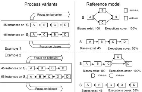
Fig. 2 depicts two very simple examples. First, consider Example 1 which shows two process variants S1 and S2. Assume that 55 process instances are running on S1and 45 instances onS2. We want to derive a generic process model such that the efforts for configuring the 100 process instances out of the generic model become minimal. If we focus on behavior, like existing process mining algorithms do63, the discovered process model will beS; all traces producible onS1andS2, respectively, can be produced on S as well, i.e. TS1 ⊆ TS and TS2 ⊆ TS. However, if we adopt S as reference model and relink process instances to it, all instances running on S1 or S2 will have a non-empty bias. More precisely, we would need to move Bin S to either obtain S1 or S2; i.e., S[σ1iS1 with σ1 =move(S,B,A,C) and S[σ2iS2
with σ2 =move(S,B,C,D) (cf. Def. 2.2). Using the number of instances as weight for each variant, average weighted distance between SandSi(i= 1,2) is one; i.e., for each process instance we need on average one high-level change operation to configureS into S1and S2respectively.
By contrast, if we focus on biases, we should chooseS0as reference model. While no adaptations become necessary for the 55 instances running on S1, we need to moveB for the 45 instances based on S2, i.e.S0[σ0iS2 with σ0 =move(S0,B,C,D).
Therefore, average weighted distance between S0 and variants Si (i = 1,2) corre- sponds to0.45. ThoughS0does not cover all traces variantsS1andS2can produce (i.e., TS2 *TS0), adapting S0 rather than S as the new generic model requires per average less efforts for process configuration, since average weighted distance be- tween S0 and the instances running on both S1 and S2 is 55% lower than when usingS.
Regarding Example 2 from the bottom of Fig. 2, activity X is only present in S2, but not in S1. When applying traditional process mining, we obtain model S (with X being contained in a conditional branch). If we want to minimize average change distance, in turn, we need to choose S0 as reference model. Note that we only consider very simple process models in Fig. 2 to illustrate basic ideas. As we show in the following, our approach works for process models with more complex structure (e.g., AND- XOR-branching and Loops) as well.
Our discussions on the difference between behavioral and structural similarity also demonstrate that current process mining algorithms do not consider struc- tural similarity based on bias and change distance. (We quantitatively compare our mining approach with existing algorithms in Section 8.) First, a fundamental requirement for traditional process mining concerns the availability of a critical number of instance traces. An alternative method is to enumerate all the traces the process variants can produce (if it is finite) to represent the process model, and to use these traces as input source (i.e., logs) for traditional process mining algorithms. Unfortunately, this does also not satisfy our need to minimize average
Example 1 Example 2
A B C D
C D
A
X B
Focus on behavior
Focus on biases S1
S2 45 instances on
55 instances on
S
S’
Biases exist: 45
A B C D
A C B D
S1
S2
A B C D
Focus on behavior
Focus on biases 55 instances on
45 instances on
A D
B
C S
S’
Biases exist: 100 Executions cover: 100%
Biases exist: 45 Executions cover: 55%
Biases exist: 100 Executions cover: 100%
Executions cover: 55%
A B C X D
Process variants Reference model
AND-Split AND-Join
XOR-Split XOR-Join
A B C X D
Fig. 2. Mining focusing either on Behavior or on Minimization of Biases
distances since it focuses on covering behavior as captured in execution logs (see Examples 1 and 2). Clearly, enumerating all the traces would be also a tedious and expensive task. For example, if a parallel branching block contains five branches and each branch contains five activities, the number of traces for such structure will be (5×5)!/(5!)5= 623360743125120.
4. Representing Block-structured Processes as Order Matrices
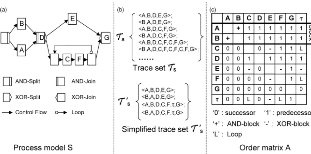
One key feature of our ADEPT change framework is to maintain the structure of the unchanged parts of a process model41,8,70. For example, if we delete an activity from a process model, the remaining process model will still be valid and the order relations (e.g., predecessor or successor) between other activities will remain the same 50,44. To incorporate this feature in our approach, rather than only looking at direct predecessor-successor relationships between activities (i.e. control edges), we consider the transitive control dependencies for each pair of activities; i.e., for a given process model S = (N, E, . . .) ∈ P, for activities ai, aj ∈ N, ai 6= aj we examine their structural order relations (including transitive one). Logically, we determine order relations by considering all traces in trace set TS producible on modelS (cf. Def. 2.3).
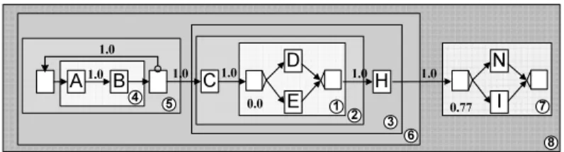
Fig. 3a shows an example of a process model S. This model is based on the patterns Sequence, AND-block, XOR-block, and Loop-block60. Here, trace setTS
ofS constitutes an infinite set due to the presence of the loop-block in S (cf. Fig.
3b). Such infinite number of traces precludes us to perform any detailed analysis of the trace set. Therefore we need to transform it into a finite representation before conducting further analysis.
4.1. Simplification of Infinite Trace Sets
One common approach to describe a string with infinite length is to represent it as finite set of n-gram lists6. General idea behind an n-gram list is to represent a single string by an ordered list of substrings with lengthn(so-calledn-grams). In partic- ular, only the first occurrence of an n-gram is considered, while later occurrences of same n-gram are omitted in the n-gram list. Thus, an n-gram list represents a collection of strings with different length. In particular, an infinite language can be represented as finite set of n-gram lists. For example, a string< abababab >can be represented as 2-gram <$a, ab, ba, b#>, where $ (#) represents the start (end) of the string. Such approach is commonly used for analyzing loop structures in pro- cess models73,3 or - more generally - in the context of text indexing for substring matching 2. Inspired by the n-gram approach, we define the notion ofSimplified Trace Set as follows:
Definition 4.1. (Simplified Trace Set) Let S be a process model and TS
denote the trace set producible on S. Let Bk, k= (1, . . . , K) be Loop-blocks inS, andTBk denote the set of traces producible by loop bodyBk. Let further(tBk)mbe a sequence ofm∈Ntraces< t1Bk, t2Bk, . . . , tmBk>with tjB
k∈ TBk,j ∈ {1, . . . , m}. We additionally define(tBk)0≡<>as empty sequence. If we only consider the activities corresponding to Bk, in any trace t ∈ TS producible on S,t either has no entries
f or must have structure < t∗Bk,(tBk)m >, with t∗Bk ∈ TBk representing the first loop iteration and m∈N0 being the number of additional iterations loop-block Bk
is executed in trace t. We can simplify this structure by using < tBk, τk >instead, whereτk refers to(tBk)m. When simplifying trace setTS this way, we obtain a finite set of traces TS0 which we denote asSimplified Trace Setof process modelS.
Order matrix A Process model S
AND-Split AND-Join
XOR-Split XOR-Join
Control Flow Loop
A A B
B C D E F G
C D E F G
1
1 1 1 1
1 1 1 1 1
1 1
1 1 1 1
1 1
0 0 0
0 0
0 0 0
0 0
0 0
0 0
0 0 0 0
+ +
-
- -
- τ
τ
1 1
1 -
0 1
0 0 L 0 - L
L
L
‘0’ : successor ‘1’ : predecessor
‘+’ : AND-block ‘-’ : XOR-block
‘L’ : Loop
<A,B,D,E,G>;
<B,A,D,E,G>;
<A,B,D,C,F,τ,G>;
<B,A,D,C,F,τ,G>
S
A C
B E
F
D G
Trace set S
Simplified trace set S
<A,B,D,E,G>;
<B,A,D,E,G>;
<A,B,D,C,F,G>;
<B,A,D,C,F,G>;
<A,B,D,C,F,C,F,G>;
<B,A,D,C,F,C,F,C,F,G>;
……
S
(a) (b) (c)
block
Fig. 3. a) Process model, b) (simplified) Trace set, and c) related order matrix
fi.e., the loop-blockBkhas not been executed at all.
In our simplified representation of a trace t ∈ TS, we only consider the first occurrence of trace t∗Bk producible by loop-block Bk, while omitting others that occur later within tracet. Instead, we represent such repetitive entries by a silent activity τk, which has no associated action, but solely exists to indicate omission of other tBk appearing later in trace t; i.e., τk represents the iterative execution of loop-blockBk as captured in tracet.g When omitting repetitive entries within trace setTS, we obtain a finite trace set TS0 that we can use for further analysis.
Note that when dealing with nested loops (e.g., a loop-blockBk contains another loop-blockBj), we first need to analyzeBj and thenBk; i.e., we need to first define τj to represent the iterative execution of loop-blockBj as captured in tracet and then we defineτk to represent loop-blockBk.
As example consider process modelSin Fig. 3a. Loop-blockB={C,F}, which is surrounded by a loop-backward edge, constitutes the block that comprises activities C and F. Consequently, the trace set this block can produce corresponds to {<
C,F >}. Therefore, when only considering activities C and F, any trace t ∈ TS
producible on S has structure < C,F,(C,F)m > with m ∈ N0 depending on the number of times the loop iterates. For example, < C,F >, < C,F,C,F > and <
C,F,C,F,C,F > are all valid traces producible by the loop-block. Let us define a silent activity τ corresponding to block B. Then we can simplify these traces by< C,F, τ > where τ refers the to the sequence of the traces producible on B.
As illustrated in Fig. 3b, we can simplify infinite trace set TS to finite set TS0 = {<A,B,D,E,G>, <B,A,D,E,G>, <A,B,D,C,F,τ,G>, <B,A,D,C,F,τ,G>}.
4.2. Representing Process Models as Order Matrices
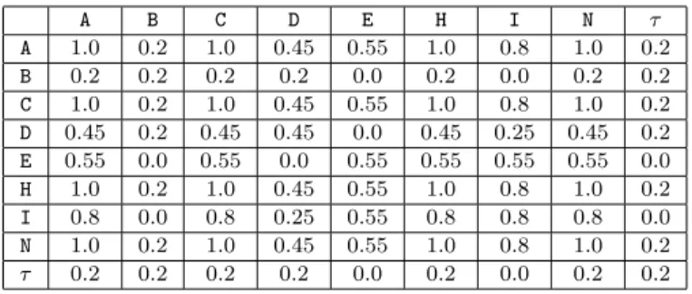
For process modelS, the analysis results concerning its trace setTS are aggregated in an order matrixA, which considers five types of order relations (cf. Def. 4.2):
Definition 4.2. (Order matrix) Let S = (N, E, . . .) ∈ P be a process model with activity set N = {a1, a2, . . . , an}. Let further TS denote the set of all traces producible on S and let TS0 be the simplified trace set of S according to Def. 4.1.
Finally let Bk, k = (1, . . . , K) denote loop-blocks in S and for every Bk, let τk, k= (1, . . . , K)be a silent activity representing the iterative structure producible by Bk inTS0. Then:
Ais calledorder matrixofSwithAaiaj representing the order relation between activitiesai,aj ∈NS
{τk
¯¯k= 1, . . . , K},i6=j iff:
• Aaiaj = ’1’ iff (∀t∈ TS0 withai, aj∈t ⇒t(ai≺aj))
If for all producible traces containing activities ai and aj, ai always appears BEFOREaj, we setAaiaj to ’1’, i.e.,ai always precedesaj in the
gThough this approach has been inspired by n-gram, it is somewhat different from n-gram rep- resentation of a string. In n-gram the length of the sub-string is a fixed numbern, while in our approach we useτkto represent traces producible by loop-blockBk. Obviously, traces producible byBkdo not need to have same length.
flow of control.
• Aaiaj = ’0’ iff (∀t∈ TS0 with ai, aj∈t⇒t(aj≺ai))
If for all producible traces containing activities ai and aj, ai always appears AFTER aj, we set Aaiaj to ’0’, i.e.ai always succeeds aj in the flow of control.
• Aaiaj = ’+’ iff (∃t1∈ TS0 withai, aj∈t1∧t1(ai≺aj))∧ (∃t2∈ TS0 with ai, aj ∈t2∧t2(aj ≺ai))
If there exists at least one producible trace in whichai appears beforeaj
and another one in whichai appears after aj, we set Aaiaj to ’+’; i.e.,ai
andaj are contained in different parallel branches.
• Aaiaj = ’-’ iff (¬∃t∈ TS0 :ai∈t∧aj ∈t)
If there is no producible trace containing both activity ai and aj, we set Aaiaj to ’-’, i.e. ai and aj are contained in different branches of a conditional branching.
• Aaiaj = ’L’, iff ((ai∈Bk∧aj=τk)∨(aj∈Bk∧ai=τk))
For any activityai in a Loop-block Bk, we define order relation Aaiτk
between it and the corresponding silent activityτk as ’L’.
The first four order relations{1,0,+,-}specify the precedence relations between activities as captured in the trace set, while the last order relation ’L’ indicates loop structures within the trace set. As example consider Fig. 3c which depicts the order matrix of process modelS. SinceS contains one loop-block, a silent activity τ is added to this order matrix as well. Note that the order matrix contains all five order relations as described in Def. 4.2. For example, activities Eand Cwill never appear in same trace of the simplified trace set, since they are contained in different branches of an XOR block. Therefore, we assign ’-’ to matrix elementAEC. Further, since in all producible traces, which contain both activityBand activityG,Balways appears beforeG, we obtain order relations ABG = ’1’ andAGB = ’0’ respectively.
Special attention should be paid to the order relations between silent activityτ and the other activities. The order relation betweenτand activitiesCandFis set to ’L’, since both CandFare contained in the loop-block; with all remaining activities τ has same order relations as C(orF) have. Note that the main diagonal of an order matrix is empty since we do not compare an activity with itself.
Generally, it is not a good idea to first enumerate all traces of a process model and then to analyze the order relations captured by them. Note that the trace set of a process model can become extremely large, particularly if the model contains multiple AND-blocks or even infinite at the presence of loop-blocks. In29, we have introduced two algorithms for transforming a block-structured process model into its corresponding order matrix and vice verse. Complexity of these two algorithms is O(2n2), wherenequals the number of activities plus the number of loop-blocks con- tained in the process model; we have further proven that an order matrix constitutes a unique representation of a block-structured process model; i.e., if we transform a process model into an order matrix and then transform the latter back into a
process model, the two process models aretrace equivalent; i.e., they cover same behavior18.
Based on an order matrix representation, we can easily identify activities belong- ing to the same block. In particular, such activities have the same order relations with respect to activities from outside this block. As example, take the order matrix depicted in Fig. 3. If we ignore the internal relation between activitiesAandB, the order relations betweenAand all other activities are the same as for B(as marked up in Fig. 3 where the first two rows are identical when ignoring the order relation betweenA and B). Based on the order matrix, we can determine a process block containingAandB. Furthermore, these activities are contained in different branches of an XOR-block (as indicated byAAB = ’-’).
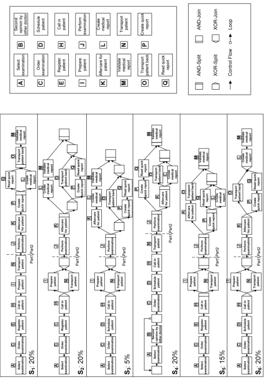
5. Hospital Case and Running Example
To illustrate our mining approach along a real-world example and to also validate it in this context, we first introduce a real-world case from one of the projects we conducted in the healthcare domain.
5.1. Case Study Description
Context.We conduct a case study in a large clinical centre (with more than 1000 beds) in Germany. In this clinical centre the diagnostic and therapeutic processes of a patient usually involve various, organizationally more or less autonomous units.
For a patient treated in a department of internal medicine or surgery, for exam- ple, tests and procedures at the laboratory and the radiology department have to be ordered. In this context, medical procedures must be planned and prepared, and appointments be made. Further, specimen or the patient himself have to be transported, physicians from other units may need to come and see the patient, and medical reports have to be written, sent, and evaluated. Thus, the cooperation between organizational units as well as the medical personnel is a vital task, with repetitive, but non-trivial character.
Data Source. We analyze several process model repositories of this clinical centre. In total, we can identify more than 90 process variants for handling med- ical orders and procedures respectively (e.g., X-ray inspections, cardiological ex- aminations). Despite their similarity the different variants are captured in sepa- rate process models based on different notations (e.g., Event-driven Process Chains and UML Activity Diagrams) and modeling components (e.g., ARIS Architect, MQSeries Workflow, ADEPT). All models use standard process patterns like Se- quence, AND-/XOR-Splits, AND-/XOR-Joins, and Loop, and their size ranges from 7 to 17 activities. Interestingly, for each non-block-structured variant model it is pos- sible to transform it into a trace equivalent, block-structured representation; i.e., it is possible to map the different variant models to a representation following our process meta model. In this context, we apply simple refactorings (e.g., relabeling of activities) in order to harmonize considered variant models67 .
Sources of Variance.Despite the structural similarity of the variant models, the latter also comprise parts only relevant for a sub-collection of the variants.
For example, some of the variants require approval of a medical order by a senior physician, while this is not required in the context of other variants. Similarly, there exist medical procedures requiring complex scheduling activities, whereas in other cases no scheduling is required or the patient simply needs to be registered at the site of the care provider. Depending on the physical condition of the treated patient, in addition, a transport may have to be organized or not. Similarly, in emergency cases a short medical report is transmitted immediately after the medical examination to the requesting unit (e.g., a ward). Other variations of the analyzed models concern the preparation phases at the site of wards and examination units respectively.
We consider the most relevant 84 process variants which make up more than 95% of the identified ones. Based on the number of corresponding process instances, we assign weights to the variant models ranging from 0.1% to 8.67%. However, none of the process variants is dominant or significantly more relevant than others.
5.2. Illustrative Example
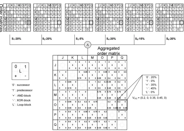
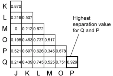
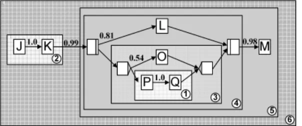
Due to space limitations, we cannot show all 84 process variants. Fig. 4 depicts six process variants Si ∈ P (i = 1,2, . . .6) from our hospital case study (to ease presentation and later discussion we assign to each labeled activity a letter ranging from AtoQ). Furthermore we assign weights to these six variant models according to their relevance. In the context of our work, we define theweightwiof a process variant Si as the percentage of process instances executed on basis of Si. In our example, 20% of instances were executed based on S1 and 5% of instances on S3. If we only know process variants, but have no runtime information about related instance executions, we will assume the variants to be equally weighted; i.e., every process variant then will have weight 1/n, where ncorresponds to the number of variants in the system.
For our following considerations, first of all, we focus on these six variants which are divided into two parts: Part2 consists of activities J,K,P,Q,L,M and O. These activities exist in all six process variantsS1-S6, but show different order relations in these variants. On the contrary, Part1 consists of activities that do not appear in all process variants. For example, activityEexists only inS1, S2andS5, but not in S3,S4 andS6.
In Section 6, we first assume that all process variants have same activity sets, i.e., we first consider solely Part2 of each process variants. In Section 7, we relax this constraint by also considering Part1 of the process variants. Finally, Section 7.5 summarizes mining results when applying our clustering algorithm to all 84 process variants from our healthcare case study.
6. Clustering Approach for Discovering Reference Process Models We now present a clustering-based algorithm for mining a collection of process variants. Our goal is to derive a new reference model out of a given collection of