Process Variants Using a Heuristic Approach

(1)

Process Variants Using a Heuristic Approach

Chen Li¹ ^?, Manfred Reichert², and Andreas Wombacher¹

1 Computer Science Department, University of Twente, The Netherlands lic@cs.utwente.nl; a.wombacher@utwente.nl

2 Institute of Databases and Information Systems, Ulm University, Germany manfred.reichert@uni-ulm.de

Abstract. Recently, a new generation of adaptive Process-Aware Infor- mation Systems (PAISs) has emerged, which enables structural process changes during runtime. Such flexibility, in turn, leads to a large number of process variants derived from the same model, but differing in structure. Generally, such variants are expensive to configure and maintain.

This paper provides a heuristic search algorithm which fosters learning from past process changes by mining process variants. The algorithm discovers a reference model based on which the need for future process configuration and adaptation can be reduced. It additionally provides the flexibility to control the process evolution procedure, i.e., we can control to what degree the discovered reference model differs from the original one. As benefit, we cannot only control the effort for updating the reference model, but also gain the flexibility to perform only the most important adaptations of the current reference model. Our mining algorithm is implemented and evaluated by a simulation using more than 7000 process models. Simulation results indicate strong performance and scalability of our algorithm even when facing large-sized process models.

1 Introduction

In today’s dynamic business world, success of an enterprise increasingly depends on its ability to react to changes in its environment in a quick, flexible and cost-effective way. Generally, process adaptations are not only needed for configuration purpose at build time, but also become necessary for single process instances during runtime to deal with exceptional situations and changing needs [11, 17]. In response to these needs adaptive process management technology has emerged [17]. It allows to configure and adapt process models at different levels.

This, in turn, results in large collections of process variants created from the same process model, but slightly differing from each other in their structure. So far, only few approaches exist, which utilize the information about these variants and the corresponding process adaptations [4].

?This work was done in the MinAdept project, which has been supported by the Netherlands Organization for Scientific Research under contract number 612.066.512.

(2)

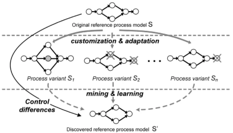
Fig. 1 describes the goal of this paper. We aim at learning from past process changes by ”merging” process variants into one generic process model, which covers these variants best. By adopting this generic model as new reference process model within the Process-aware Information System (PAIS), need for future process adaptations and thus cost for change will decrease. Based on the two assumptions that (1) process models are well-formed (i.e., block-structured like in WS-BPEL) and (2) all activities in a process model have unique labels, this paper deals with the following fundamental research question:Given a reference model and a collection of process variants configured from it, how to derive a new reference process model by performing a sequence of change operations on the original one, such that the average distance between the new reference model and the process variants becomes minimal?

…

Original reference process model ^S customization & adaptation

Process variant S₁ Process variant S₂ Process variant S_n mining & learning

Discovered reference process model ^S’

Control differences

Fig. 1.Discovering a new reference model by learning from past process configurations The distance between the reference process model and a process variant is measured by the number of high-level change operations (e.g., to insert, delete or move activities [11]) needed to transform the reference model into the variant.

Clearly, the shorter the distance is, the less the efforts needed for process adaptation are. Basically, we obtain a new reference model by performing a sequence of change operations on the original one. In this context, we provide users the flexibility to control the distance between old reference model and newly discovered one, i.e., to choose how many change operations shall be applied. Clearly, the most relevant changes (which significantly reduce the average distance) should be considered first and the less important ones last. If users decide to ignore less relevant changes in order to reduce the efforts for updating the reference model, overall performance of our algorithm with respect to the described research goal is not influenced too much. Such flexibility to control the difference between the original and the discovered model is a significant improvement when compared to our previous work [5, 9].

Section 2 gives background information for understanding this paper. Section 3 introduces our heuristic algorithm and provides an overview on how it can be used for mining process variants. We describe two important aspects of our

(3)

heuristics algorithm (i.e., fitness function and search tree) in Sections 4 and 5.

To evaluate its performance, we conduct a simulation in Section 6. Section 7 discusses related work and Section 8 concludes with a summary.

2 Backgrounds

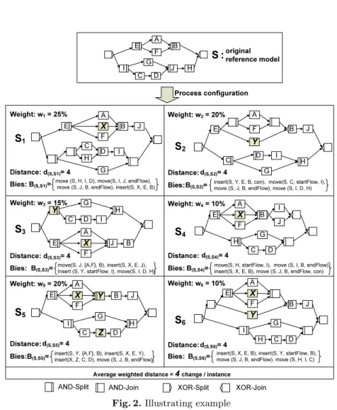
Process Model. Let P denote the set of all sound process models. A particular process model S = (N, E, . . .) ∈ P is defined as Well-structured Activity Net³[11].Nconstitutes the set of process activities andEthe set of control edges (i.e., precedence relations) linking them. To limit the scope, we assume Activity Nets to be block-structured (like BPEL). Examples are depicted in Fig. 2.

Process change. Aprocess change is accomplished by applying a sequence of change operations to the process modelSover time [11]. Such change operations modify the initial process model by altering the set of activities and their order relations. Thus, each application of a change operation results in a new process model. We define process change andprocess variants as follows:

Definition 1 (Process Change and Process Variant). Let P denote the set of possible process models and C be the set of possible process changes. Let S, S⁰ ∈ P be two process models, let ∆ ∈ C be a process change expressed in terms of a high-level change operation, and let σ =h∆1, ∆2, . . . ∆ni ∈ C^∗ be a sequence of process changes performed on initial model S. Then:

– S[∆iS⁰ iff∆is applicable toS andS⁰ is the (sound) process model resulting from application of∆ toS.

– S[σiS⁰ iff ∃ S1, S2, . . . Sn+1 ∈ P with S = S1, S⁰ =Sn+1, and Si[∆iiSi+1

fori∈ {1, . . . n}. We denote S⁰ as variant of S.

Examples of high-level change operations includeinsert activity, delete ac- tivity, andmove activity as implemented in the ADEPT change framework [11].

Whileinsert anddelete modify the set of activities in the process model,move changes activity positions and thus the order relations in a process model. For example, operation move(S,A,B,C) shifts activity A from its current position within process model S to the position after activity B and before activity C.

Operation delete(S,A), in turn, deletes activityAfrom process modelS. Issues concerning the correct use of these operations, their generalizations, and formal pre-/post-conditions are described in [11]. Though the depicted change operations are discussed in relation to our ADEPT approach, they are generic in the sense that they can be easily applied in connection with other process meta models as well [17]; e.g., life-cycle inheritance known from Petri Nets [15]. We refer to ADEPT since it covers by far most high-level change patterns and change support features [17], and offers a fully implemented process engine.

3 A formal definition of a Well-structured Activity Net contains more than only node setNand edge setE. We omit other components since they are not relevant in the given context [18].

(4)

Definition 2 (Bias and Distance). Let S, S⁰ ∈ P be two process models.

Distanced_(S,S⁰₎between S andS⁰ corresponds to the minimal number of high- level change operations needed to transformS intoS⁰; i.e., we define d_(S,S⁰₎:=

min{|σ| | σ ∈ C^∗∧S[σiS⁰}. Furthermore, a sequence of change operations σ with S[σiS⁰ and|σ|=d_(S,S⁰₎ is denoted asbias B_(S,S⁰₎ betweenS andS⁰.

Thedistance betweenS andS⁰ is the minimal number of high-level change operations needed for transforming S into S⁰. The corresponding sequence of change operations is denoted as bias B_(S,S⁰₎ betweenS and S⁰.⁴ Usually, such distance measures the complexity for model transformation (i.e., configuration).

As example take Fig. 2. Here, distance between modelSand variantS1is 4, i.e., we minimally need to perform 4 changes to transform S into S⁰ [7]. In general, determining bias and distance between two process models has complexity at N P −hardlevel [7]. We consider high-level change operations instead of change primitives (i.e., elementary changes like adding or removing nodes / edges) to measure distance between process models. This allows us to guarantee soundness of process models and provides a more meaningful measure for distance [7, 17].

Trace. A trace t on process model S = (N, E, . . .) ∈ P denotes a valid and complete execution sequencet≡< a1, a2, . . . , ak >of activityai ∈N according to the control flow set out by S. All traces S can produce are summarized in trace setTS.t(a≺b) is denoted as precedence relation between activitiesaand b in tracet≡< a1, a2, . . . , ak >iff∃i < j :ai=a∧aj=b.

Order Matrix. One key feature of any change framework is to maintain the structure of the unchanged parts of a process model [11]. To incorporate this in our approach, rather than only looking at direct predecessor-successor relation between activities (i.e., control edges), we consider the transitive control depen- dencies for each activity pair; i.e., for given process modelS = (N, E, . . .)∈ P, we examine for every pair of activitiesai, aj ∈N,ai6=aj their transitive order relation. Logically, we determine order relations by considering all traces the process model can produce. Results are aggregated in an order matrixA|N|×|N|, which considers four types of control relations (cf. Def. 3):

Definition 3 (Order matrix). Let S = (N, E, . . .) ∈ P be a process model with N ={a1, a2, . . . , an}. Let furtherTS denote the set of all traces producible onS. Then: MatrixA_|N|×|N| is calledorder matrixofS withAij representing the order relation between activitiesai,aj ∈N,i6=j iff:

– Aij= ’1’ iff [∀t∈ TS withai, aj∈t⇒t(ai≺aj)]. If for all traces containing activitiesai and aj,ai always appears BEFORE aj, we denoteAij as ’1’, i.e.,ai always precedes aj in the flow of control.

– Aij= ’0’ iff [∀t∈ TS withai, aj ∈t⇒t(aj ≺ai)]. If for all traces containing activitiesai andaj,ai always appears AFTER aj, we denoteAij as a ’0’, i.e.ai always succeedsaj in the flow of control.

4 Generally, it is possible to have more than one minimal set of change operations to transformSintoS⁰, i.e., given process modelsS andS⁰their bias does not need to be unique. A detailed discussion of this issue can be found in [15, 7].

(5)

– Aij = ’*’ iff [∃t1 ∈ TS, with ai, aj ∈ t1∧t1(ai ≺ aj)] ∧ [∃t2 ∈ TS, with ai, aj∈t2∧t2(aj ≺ai)]. If there exists at least one trace in whichai appears beforeaj and another trace in which ai appears after aj, we denote Aij as

’*’, i.e.ai andaj are contained in different parallel branches.

– Aij = ’-’ iff [¬∃t ∈ TS : ai ∈ t∧aj ∈ t]. If there is no trace containing both activityai andaj, we denote Aij as ’-’, i.e. ai andaj are contained in different branches of a conditional branching.

Given a process model S = (N, E, . . .) ∈ P, the complexity to compute its order matrix A|N|×|N| isO(2|N|²) [7]. Regarding our example from Fig. 2, the order matrix of each process variantSiis presented on the top of Fig. 4.⁵Variants Si contain four kinds of control connectors: AND-Split, AND-Join, XOR-Split, and XOR-join. The depicted order matrices represent all possible order relations.

As example considerS4. ActivitiesHandInever appear in same trace since they are contained in different branches of an XOR block. Therefore, we assign ’-’ to matrix elementAHI forS4. If certain conditions are met, the order matrix can uniquely represent the process model. Analyzing its order matrix (cf. Def. 3) is then sufficient in order to analyze the process model [7].

It is also possible to handle loop structures based on an extension of order matrices, i.e., we need to introduce two additional order relations to cope with loop structures in process models [7]. However, since activities within a loop structure can run an arbitrarily number of times, this complicates the definition of order matrix in comparison to Def. 3. In this paper, we use process models without loop structures to illustrate our algorithm. It will become clear in Section 4 that our algorithm can easily be extended to also handle process models with loop structures by extending Def. 3.

3 Overview of our Heuristic Search Algorithm

Running Example. An example is given in Fig. 2. Out of original reference model S, six different process variants Si ∈ P (i = 1,2, . . .6) are configured.

These variants do not only differ in structure, but also in their activity sets. For example, activity Xappears in 5 of the 6 variants (exceptS2), whileZonly appears inS5. The 6 variants are further weighted based on the number of process instances created from them; e.g., 25% of all instances were executed according to variantS1, while 20% ran onS2. We can also compute the distance (cf. Def.

2) between S and each variant Si. For example, when comparing S with S1

we obtain distance 4 (cf. Fig. 2); i.e., we need to apply 4 high-level change operations [move(S,H,I,D), move(S,I,J, endF low), move(S,J,B, endF low) and insert(S,X,E,B)] to transformSintoS1. Based on weightwiof each variantSi, we can compute average weighted distance between reference model S and its variants. As distances between S and Si we obtain 4 for i = 1, . . . ,6 (cf. Fig.

2). When considering variant weights, as average weighted distance, we obtain 4×0.25 + 4×0.2 + 4×0.15 + 4×0.1 + 4×0.2 + 4×0.1 = 4.0. This means we need to perform on average 4.0 change operations to configure a process variant (and

5 Due to lack of space, we only depict order matrices for activitiesH,I,J,X,YandZ.

(6)

Process configuration original reference model

S₁

S₂

S₃ S₄

S₅

S₆

Average weighted distance = 4 change / instance G

E B

I J

A F

C D H

E Y B J

I G H

C Z D

A F X

G

E B

A

F I

X J

C D H

H G

C D

E B I

J A

F X

Y G H

C D

B I

E J

A F X Distance: d(S,S1)= 4

Distance: d(S,S3)= 4

d(S,S5)= 4 d(S,S6)= 4

d(S,S4)= 4 d(S,S2)= 4

insert(S, X, E, B), insert(S, Y, startFlow, B), move (S, J, B, endFlow), move (S, H, I, C) B(S,S6)=

insert(S, Y, {A,F}, B), insert(S, X, E, Y), insert(X, Z, C, D), move (S, J, B, endFlow) B(S,S5)=

move(S, J, {A,F}, B), insert(S, X, E, J), Insert (S, Y, startFlow, I), move(S, I, D, H) B(S,S3)=

insert(S, Y, E, B, con), move(S, C, startFlow, I), move (S, J, B, endFlow), move (S, I, D, H) B(S,S2)=

move(S, H, startFlow, I), move (S, I, B, endFlow), insert(S, X, E, B), move (S, J, B, endFlow, con) B(S,S4)=

D A F

I

E B

Y

J

G

C H

E

B

Y ^J

I G

H C D

A F X

AND-Split AND-Join XOR-Split XOR-Join

S :

Weight: w1= 25%

Weight: w3= 15%

Weight: w5= 20%

Weight: w2= 20%

Weight: w4= 10%

Weight: w6= 10%

move (S, H, I, D), move(S, I, J, endFlow), move (S, J, B, endFlow), insert(S, X, E, B) Bies: B(S,S1)=

Bies:

Bies: Bies:

Bies:

Distance: Distance:

Distance:

Fig. 2.Illustrating example

related instance respectively) out ofS. Generally,average weighted distance between a reference model and its process variants represents how ”close” they are.

The goal of our mining algorithm is to discover a reference model for a collection of (weighted) process variants with minimal average weighted distance.

Heuristic Search for Mining Process Variants.As measuring distance between two models hasN P −hardcomplexity (cf. Def. 2), our research question (i.e., finding a reference model with minimal average weighted distance to the variants), is a N P −hard problem as well. When encountering real-life cases, finding ”the optimum” would be either too time-consuming or not feasible. In this paper, we therefore present aheuristic search algorithmfor mining variants.

Heuristic algorithms are widely used in various fields, e.g., artificial intelligence [10] and data mining [14]. Although they do not aim at finding the ”real optimum” (i.e., it is neither possible to theoretically prove that discovered results are optimal nor can we say how close they are to the optimum), they are

(7)

constraintNo

S_nc: Search result without constraint

S_i_:Variants

d=1

d = 2 d = 3

S: Original reference

model

Discovered Reference Model Original

Reference model Process

variants Intermediate

search result Search

steps S_c: Search result

with constraint Force 1:

close to variants Force 2:

close to reference

Fig. 3.Our heuristic search approach

widely used in practice. Particularly, they can nicely balance goodness of the discovered solution and time needed for finding it [10].

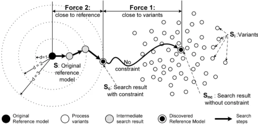
Fig. 3 illustrates how heuristic algorithms can be applied for the mining of process variants. Here we represent each process variantSi as single node (white node). The goal for variant mining is then to find the ”center” of these nodes (bull’s eye Snc), which has minimal average distance to them. In addition, we want to take original reference modelS (solid node) into account, such that we can control the difference between the newly discovered reference model and the original one. Basically, this requires us to balance two forces: one is to bring the newly discovered reference model closer to the variants; the other one is to

”move” the discovered model not too far away fromS. Process designers should obtain the flexibility to discover a model (e.g., Sc in Fig. 3), which is closer to the variants on the one hand, but still within a limited distance to the original model on the other hand.

Our heuristic algorithm works as follows: First, we use original reference modelS as starting point. AsStep 2, we search for all neighboring models with distance 1 to the currently considered reference process model. If we are able to find a model Sc with lower average weighted distance to the variants, we replace S by Sc. We repeat Step 2 until we either cannot find a better model or the maximally allowed distance between original and new reference model is reached.

For any heuristic search algorithm, two aspects are important: theheuristic measure (cf. Section 4) and the algorithm (Section 5) that uses heuristics to search the state space.

4 Fitness Function of our Heuristic Search Algorithm

Any fitness function of a heuristic search algorithm should be quickly computable. Average weighted distance itself cannot be used as fitness function, since complexity for computing it isN P −hard. In the following, we introduce a fitness function computable in polynomial time, to approximately measure

”closeness” between a candidate model and the collection of variants.

(8)

4.1 Activity Coverage

For a candidate process model Sc = (Nc, Ec, . . .) ∈ P, we first measure to what degree its activity setNccovers the activities that occur in the considered collection of variants. We denote this measure asactivity coverageAC(Sc) ofSc. Before we can compute it, we first need to determine activity frequency g(aj) with which each activityaj appears within the collection of variants. LetSi∈ P i= 1, . . . , nbe a collection of variants with weightswi and activity setsNi. For eachaj ∈S

Ni, we obtain g(aj) =P

Si:aj∈Niwi. Table 1 shows the frequency of each activity contained in any of the variants in our running example; e.g.,X is present in 80% of the variants (i.e., in S₁, S₃, S₄, S₅, andS₆), while Zonly occurs in 20% of the cases (i.e., inS5).

ActivityA B C D E F G H I J X Y Z

g(aj) 1 1 1 1 1 1 1 1 1 1 0.8 0.65 0.2

Table 1.Activity frequency of each activity within the given variant collection LetM =S_n

i=1Ni be the set of activities which are present in at least one variant. Given activity frequencyg(aj) of eachaj∈M, we can computeactivity coverage AC(Sc) of candidate modelSc as follows:

AC(Sc) = P

aj∈Ncg(aj) P

aj∈Mg(aj) (1)

The value range ofAC(Sc) is [0,1]. Let us take original reference model S as candidate model. It contains activitiesA, B, C, D, E, F, G, H, I, andJ, but does not containX, YandZ. Therefore, its activity coverageAC(S) is 0.858.

4.2 Structure Fitting

ThoughAC(Sc) measures how representative the activity setNc of a candidate model Sc is with respect to a given variant collection, it does not say anything about the structure of the candidate model. We therefore introduce structure fittingSF(Sc), which measures, to what degree a candidate modelScstructurally fits to the variant collection. We first introduce aggregated order matrix and coexistence matrix to adequately represent the variants.

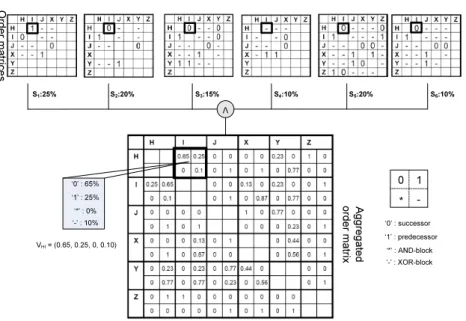
Aggregated Order Matrix.For a given collection of process variants, first, we compute the order matrix of each process variant (cf. Def. 3). Regarding our running example from Fig. 2, we need to compute six order matrices (see to of Fig. 4). Note that we only show a partial view on the order matrices here (activitiesH, I, J, X, YandZ) due to space limitations. As the order relation between two activities might be not the same in all order matrices, this analysis does not result in a fixed relation, but provides a distribution for the four types of order relations (cf. Def. 3). Regarding our example, in 65% of all cases H succeedsI(as in S2,S3,S4 andS6), in 25% of all casesHprecedesI(as inS1), and in 10% of all casesHand Iare contained in different branches of an XOR

(9)

0 1

* -

‘0’ : successor

‘1’ : predecessor

‘*’ : AND-block

‘-’ : XOR-block

Order matrices Aggregatedorder matrix

V

S₁:25% S₂:20% S₃:15% S₄:10% S₅:20% S₆:10%

VH I= (0.65, 0.25, 0, 0.10)

‘0’ : 65%

‘1’ : 25%

‘*’ : 0%

‘-’ : 10%

Fig. 4.Aggregated order matrix based on process variants

block (as in S4) (cf. Fig. 4). Generally, for a collection of process variants we can define the order relation between activitiesaandbas 4-dimensional vector V_ab = (v⁰_ab, v¹_ab, v_ab^∗ , v⁻_ab). Each field then corresponds to the frequency of the respective relation type (’0’, ’1’, ’*’ or ’-’) as specified in Def. 3. For our example from Fig. 2, for instance, we obtainVHI = (0.65,0.25,0,0.1) (cf. Fig. 4). Fig. 4 shows aggregated order matrixV for the process variants from Fig. 2.

Coexistence Matrix.Generally, the order relations computed by an aggregated order matrix may not be equally important; e.g., relationshipVHIbetween H and I (cf. Fig. 4) would be more important than relation VHZ, since H and I appear together in all six process variants while H and Z only show up together in variant S5 (cf. Fig. 2). We therefore define Coexistence Matrix CE in order to represent the importance of the different order relations occurring within an aggregated order matrix V. Let Si (i = 1. . . n) be a collection of

Fig. 5.Coexistence Matrix

(10)

process variants with activity sets Ni and weight wi. The Coexistence Matrix of these process variants is then defined as 2-dimensional matrixCEm×m with m =|S

Ni|. Each matrix elementCEjk corresponds to the relative frequency with which activities aj and ak appear together within the given collection of variants. Formally:∀aj, ak∈S

Ni, aj6=ak :CEjk=P

Si:aj∈Ni∧ak∈Niwi. Table 5 shows the coexistence matrix for our running example (partial view).

Structure Fitting SF(Sc) of Candidate Model Sc. Since we can represent candidate process model Sc by its corresponding order matrixAc (cf. Def.

3), we determinestructure fitting SF(Sc) betweenSc and the variants by measuring how similar order matrixAcand aggregated order matrixV (representing the variants) are. We can evaluateSc by measuring the order relations between every pair of activities in Ac and V. When considering reference model S as candidate process model Sc (i.e.,Sc =S), for example, we can build an aggre- gated order matrix V^c purely based onSc, and obtainVHI^c = (1,0,0,0); i.e., H always succeedsI. Now, we can compareVHI= (0.65,0.25,0,0.1) (representing the variants) andVHI^c (representing the candidate model).

We use Euclidean metricsf(α, β) to measure closeness between vectorsα= (x₁, x₂, ..., x_n) andβ = (y₁, y₂, ..., y_n):f(α, β) = _|α|×|β|^α·β =

P_n

i=1xiyi

√P_n

i=1x²_i×√P_n

i=1y²_i. f(α, β)∈[0,1] computes the cosine value of the angleθ between vectorsαand β in Euclidean space. The higher f(α, β) is, the moreα and β match in their directions. Regarding our example we obtain f(VHI, VHI^c ) = 0.848. Based on f(α, β), which measuressimilaritybetween the order relations inV (representing the variants) and inV^c (representing candidate model), and Coexistence matrix CE, which measuresimportanceof the order relations, we can computestructure fitting SF(S_c) of candidate modelS_c as follows:

SF(Sc) = P_n

j=1

P_n

k=1,k6=j[f(Vajak, V_a^c_j_a_k)·CEajak]

n(n−1) (2)

n=|Nc|corresponds to the number of activities in candidate modelSc. For every pair of activitiesaj, ak ∈Nc, j6=k, we compute similarity of corresponding order relations (as captured by V andVc) by means off(Vajak, V_a^c_j_a_k), and the importance of these order relations byCEajak. Structure fittingSF(Sc)∈[0,1]

of candidate model Sc then equals the average of the similarities multiplied by the importance of every order relation. For our example from Fig. 2, structure fittingSF(S) of original reference modelS is 0.749.

4.3 Fitness Function

So far, we have described the two measurements activity coverageAC(Sc) and structure fitting SF(Sc) to evaluate a candidate model Sc. Based on them, we can computefitnessF it(Sc) ofSc : F it(Sc) =AC(Sc)×SF(Sc).

As AC(Sc) ∈ [0,1] and SF(Sc) ∈ [0,1], value range of F it(Sc) is [0,1] as well. Fitness value F it(Sc) indicates how ”close” candidate model Sc is to the given collection of variants. The higherF it(Sc) is, the closerScis to the variants and the less configuration efforts are needed. Regarding our example from Fig.

(11)

2, fitness value F it(S) of the original reference process modelS corresponds to F it(S) =AC(S)×SF(S) = 0.858×0.749 = 0.643.

5 Constructing the Search Tree

5.1 The Search Tree

Let us revisit Fig. 3, which gives a general overview of our heuristic search approach. Starting with the current candidate model Sc, in each iteration we search for its direct ”neighbors” (i.e., process models which have distance 1 to Sc) trying to find a better candidate modelS⁰_cwith higher fitness value. Generally for a given process model Sc, we can construct a neighbor model by applying ONE insert, delete, or move operation to Sc. All activities aj ∈ S

Ni, which appear at least in one variant, are candidate activities for change. Obviously, an insert operation adds a new activity aj ∈/ Nc to Sc, while the other two operations delete or move an activitya_j already present in S_c (i.e.,a_j∈N_c).

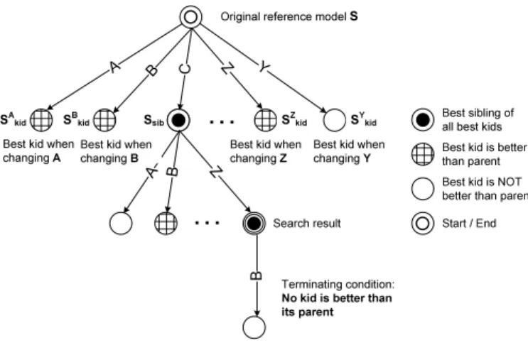
Generally, numerous process models may result by changing one particular activityajonSc. Note that the positions where we can insert (aj∈/ Nc) or move (aj ∈ Nc) activityaj can be numerous. Section 5.2 provides details on how to find all process models resulting from the change of one particular activity a_j on Sc. First of all, we assume that we have already identified these neighbor models, including the one with highest fitness value (denoted as the best kid S_kid^j ofSc when changingaj). Fig. 6 illustrates our search tree (see [8] for more details). Our search algorithm starts with setting the original reference model S as the initial state, i.e., Sc =S (cf. Fig. 6). We further define AS as active activity set, which contains all activities that might be subject to change. At the beginning,AS={aj|aj∈S_n

i=1Ni}contains all activities that appear in at least one variantSi. For each activityaj∈AS, we determine the corresponding best kidS_kid^j ofSc. IfS_kid^j has higher fitness value thanSc, we mark it; otherwise, we remove aj from AS (cf. Fig. 6). Afterwards, we choose the model with highest

Ssib

S^Bkid

S^Akid

…

A B C YZ

Best kid when changing A

A B Z

…

Best kid when

changing Z Best kid when changing Y

Best kid when changing B

Best sibling of all best kids

B

Best kid is better than parent Best kid is NOT better than parent

Terminating condition:

No kid is better than its parent

Start / End Original reference model S

Search result

S^Zkid S^Ykid

Fig. 6.Constructing the search tree

(12)

fitness valueS_kid^j∗ among all best kidsS_kid^j , and denote this model asbest sibling Ssib. We then setSsib as the first intermediate search result and replaceSc by Ssib for further search. We also removeaj∗ from AS since it has been already considered.

The described search method goes on iteratively, until termination condition is met, i.e., we either cannot find a better model or the allowed search distance is reached. The final search result Ssib corresponds to our discovered reference model S⁰ (the node marked by a bull’s eye and circle in Fig. 6).

5.2 Options for Changing One Particular Activity

Section 5.1 has shown how to construct a search tree by comparing the best kids S_kid^j . This section discusses how to find such best kidS^j_kid, i.e., how to find all

”neighbors” of candidate model Sc by performing one change operation on a particular activity aj. Consequently, S_kid^j is the one with highest fitness value among all considered models. Regarding a particular activity aj, we consider three types of basic change operations: delete, move and insert activity. The neighbor model resulting through deletion of activityaj ∈Nc can be easily determined by removing aj from the process model and the corresponding order matrix [7]; furthermore, movement of an activity can be simulated by its deletion and subsequent re-insertion at the desired position. Thus, the basic challenge in finding neighbors of a candidate modelScis to apply one activityinsertionsuch thatblock structuring andsoundness of the resulting model can be guaranteed.

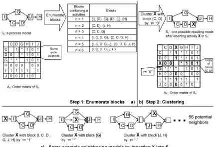
Obviously, the positions where we can (correctly) insertaj into Sc are our sub- jects of interest. Fig. 7 provides an example. Given process modelSc, we would like to find all process models that may result when inserting activityXintoSc. We apply the following two steps to ”simulate” the insertion of an activity.

Step 1 (Block-enumeration):First, we enumerate all possible blocks the candidate modelSc contains. A block can be an atomic activity, a self-contained part of the process model, or the process model itself. LetScbe a process model with activity set Nc = {a1, . . . , an} and let further Ac be the order matrix of Sc. Two activitiesai andaj can form a block if and only if [∀ak∈Nc\ {ai, aj}: Aik=Ajk] holds (i.e., iff they have exactly same order relations to the remaining activities). Consider our example from Fig. 7a. Here Cand D can form a block {C, D}since they have same order relations to remaining activitiesG, H, Iand J. In our context, we consider each block as set rather than as process model, since its structure is evident inSc. As extension, two blocksBjandBkcan merge into a bigger one iff [(a_α, a_β, a_γ)∈B_j×B_k×(N\B_jS

B_k) :A_αγ =A_βγ] holds;

i.e., two blocks can merge into a bigger block iff all activitiesaα∈Bj, aβ∈Bk

show same order relations to the remaining activities outside the two blocks. For example, block {C, D} and block{G} show same order relations in respect to remaining activities H, IandJ; therefore they can form a bigger block{C, D, J}. Fig. 7a shows all blocks contained inSc (see [8] for a detailed algorithm).

Step 2 (Cluster Inserted Activity with One Block): Based on the enumerated blocks, we describe where we can (correctly) insert a particular activityaj inSc. Assume that we want to insertXinSc (cf. Fig. 7b). To ensure

(13)

a) b) Step 1: Enumerate blocks

I G J

C D H

{C, D}, {J, H}

{C, D, G}

{I, C, D, G}, {C, D, G, H}

Blocks containing n

activities n = 1 n = 2 n = 3 n = 4 n = 5 n = 6

{I}, {G}, {C}, {D}, {J}, {H}

{I, C, D, G, J}, {C, D, G, J, H}

{I, C, D, G, J, H}

Blocks Enumerate

blocks Sc: a process model

Cluster X with block {C, D}

by τ= “0”

Sc’: one possible resulting model after inserting activity X in Sc

C D G H I J

CD

GH JI

**

* * 00 00 0 0

0 0 0

1 1

0 1

1 1

1 1 1

X

1 X

* 10 1 0*

01 0 0

11

τ= “0”

Copy block of {C,D}

C D G H I J CD

GH JI

1 1 1

11 11

11 1 1 1 1

0 0

00 0 0 0 0 0 0 0 0 0

**

* *

Same order relations

Ac: Order matrix of Sc

AS’: Order matrix of Sc’ Step 2: Clustering

I G J

C D H

X

56 potential neighbors Cluster X with block {I, C, D,

G, J, H} by τ= “1” Cluster X with block {G}

by τ= “*”

G X

I C D J H

G

I X J H

C D

I G J

C D H

X

Cluster X with block {J, H}

by τ= “-”

Some example neighboring models by inserting X into Sc

c)

Fig. 7.Finding the neighboring models by insertingXinto process modelS the block structure of the resulting model, we ”cluster”X with an enumerated block, i.e., we replace one of the previously determined blocks B by a bigger block B⁰ that containsB as well as X. In the context of this clustering, we set order relations betweenXand all activities in blockB asτ∈ {0,1,∗,−}(cf Def.

3). One example is given in Fig. 7b. Here inserted activity X is clustered with block {C, D} by order relationτ = ”0”, i.e., we setXas successor of the block containing C and D. To realize this clustering, we have to set order relations betweenXon the one hand and activitiesCandDfrom the selected block on the other hand to ”0”. Furthermore, order relations between X and the remaining activities are same as for {C, D}. Afterwards these three activities form a new block{C, D, X}replacing the old one{C, D}. This way, we obtain a sound and block-structured process modelS_c⁰ by insertingXintoSc.

We can guarantee that the resulting process model is sound and block- structured. Every time we cluster an activity with a block, we actually add this activity to the position where it can form a bigger block together with the selected one, i.e., we replace a self-contained block of a process model by a bigger one. Obviously, S_c⁰ is not the only neighboring model of Sc. For each block B enumerated in Step 1, we can cluster it withXby any one of the four order rela- tionsτ∈ {0,1,∗,−}. Regarding our example from Fig. 7,S contains 14 blocks.

Consequently, the number of models that may result when addingXtoSc equals 14×4 = 56; i.e., we can obtain 56 potential models by inserting XintoSc. Fig.

7c shows some neighboring models ofSc.

5.3 Search Result for our Running Example

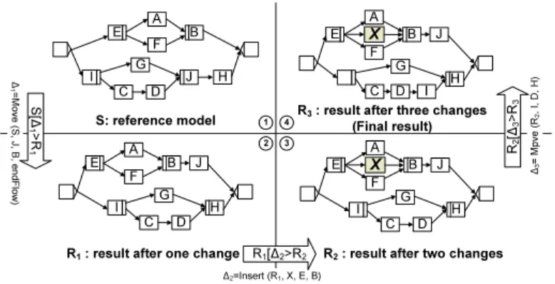
Regarding our example from Fig. 2, we now present the search result and all intermediate models we obtain when applying our algorithm (see Fig. 8).

(14)

The first operation∆1 =move(S,J,B, endF low) changes original reference model S into intermediate result model R1 which is the one with highest fitness value among all neighboring models of S. Based on R1, we discover R2

by change ∆2 =insert(R1,X, E, B), and finally we obtain R3 by performing change ∆3=move(R2,I,D,H) on R2. Since we cannot find a ”better” process model by changing R3 anymore, we obtain R3 as final result. Note that if we only allow to change original reference model by maximaldchange operations, the final search result would be: Rd if d≤3 or R3 ifd≥4.

G

E B

I J

A F

C D H

G

E B

I H

A F

C D

J

G

E B

H A

F C D X J

I

G

E B

I H

A F

C D

X J S: reference model

1∆=M ove ( S, J , B, e ndFlo w) S[∆1

>R

1

R1: result after one change R2: result after two changes R3: result after three changes

(Final result)

∆2=Insert (R1, X, E, B) R1[∆2>R2

∆³

= M pve (R² , I, D , H )

R²[∆³>R³

1

2 3

4

Fig. 8.Search result after every change

We further compare original reference modelS and all (intermediate) search results in Fig. 9. As our heuristic search algorithm is based on finding process models with higher fitness values, we observe improvements of the fitness values for each search step. Since such fitness value is only a ”reasonable guessing”, we also compute average weighted distance between the discovered model and the variants, which is a precise measurement in our context. From Fig. 9, average weighted distance also drops monotonically from 4 (when consideringS) to 2.35 (when consideringR3).

Additionally, we evaluatedelta-fitnessanddelta-distance, which indicate relative change of fitness and average weighted distance for every iteration of the algorithm. For example,∆1changesSintoR1. Consequently, it improves fitness value (delta-fitness) by 0.0171 and reduces average weighted distance (delta- distance) by 0.8. Similarly, ∆2 reduces average weighted distance by 0.6 and

∆₃ by 0.25. The monotonic decrease of delta-distance indicates that important changes (reducing average weighted distance between reference model and variants most) are indeed discovered at beginning of the search.

Another important feature of our heuristic search is its ability to automatically decide on which activities shall be included in the reference model. A predefined threshold or filtering of the less relevant activities in the activity set is not needed; e.g., Xis automatically inserted, butYandZare not added. The three change operations (insert, move, delete) are automatically balanced based on their influence on the fitness value.

(15)

5.4 Proof-of-Concept Prototype

The described approach has been implemented and tested using Java. We use our ADEPT2 Process Template Editor [12] as tool for creating process variants.

For each process model, the editor can generate an XML representation with all relevant information (like nodes, edges, blocks). We store created variants in a variants repository which can be accessed by our mining procedure. The mining algorithm has been developed as stand-alone service which can read the original reference model and all process variants, and generate the result models according to the XML schema of the process editor. All (intermediate) search results are stored and can be visualized using the editor.

6 Simulation

Of course, using one example to measure the performance of our heuristic mining algorithm is far from being enough. Since computing average weighted distance is atN P −hardlevel, fitness function is only an approximation of it. Therefore, the first question isto what degree delta-fitness is correlated with delta-distance?

In addition, we are interested in knowing to what degree important change operations are performed at the beginning. If biggest distance reduction is obtained with the first changes, setting search limitations or filtering out the change operations performed at the end, does not constitute a problem. Therefore, the second research question is: To what degree are important change operations positioned at the beginning of our heuristic search?

We try to answer these questions usingsimulation; i.e., by generating thou- sands of data samples, we can provide a statistical answer for these questions. In our simulation, we identify several parameters (e.g., size of the model, similarity of the variants) for which we investigate whether they influence the performance of our heuristic mining algorithm (see [8] for details). By adjusting these parameters, we generate 72 groups of datasets (7272 models in total) covering different scenarios. Each group contains a randomly generated reference process model and a collection of 100 different process variants. We generate each variant by configuring the reference model according to a particular scenario.

We perform our heuristic mining to discover new reference models. We do not set constraints on search steps, i.e., the algorithm only terminates if no better model can be discovered.All (intermediate) process modelsare documented (see Fig. 8 as example). We compute the fitness and average weighted distance of each intermediate process models as obtained from our heuristic mining. We

S R1 R2 R3

0.643 0.814 0.854 0.872 4 3.2 2.6 2.35

0.171 0.04 0.017 0.8 0.6 0.25 Fitness

Average weighted distance Delta-fitness Delta-distance

Fig. 9.Evaluation of the search results

(16)

Fig. 10.Execution time and correlation analysis of groups with different sizes additionally compute delta-fitness and delta-distance in order to examine the influence of every change operation (see Fig. 9 for an example).

Improvement on average weighted distances. In 60 (out of 72) groups we are able to discover a new reference model. The average weighted distance of the discovered model is0.765 lower than the one of the original reference model;

i.e., we obtain a reduction of17.92% on average.

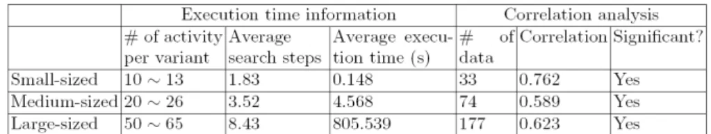
Execution time. The number of activities contained in the variants can significantly influence execution time of our algorithm. Search space becomes larger for bigger models since the number of candidate activities for change and the number of blocks contained in the reference model become higher. The average run time for models of different size is summarized in Fig. 10.

Correlation of delta-fitness and delta-distance. One important issue we want to investigate is how delta-fitness is correlated to delta-distance. Ev- ery change operation leads to a particular change of the process model, and consequently creates a delta-fitness xi and delta-distance yi. In total, we have performed284 changes in our simulation when discovering reference models. We use Pearson correlation to measure correlation between delta-fitness and delta- distance [13]. LetX be delta-fitness and Y be delta-distance. We obtainndata samples (xi, yi),i= 1, . . . , n. Let ¯xand ¯y be the mean ofX and Y, and letsx

andsy be the standard deviation ofX andY. The Pearson correlationrxy then equalsrxy=

Pxiyi−n¯x¯y

(n−1)sxsy [13]. Results are summarized in Fig. 10. All correlation coefficients are significant and high (> 0.5). The high positive correlation between delta-fitness and delta-distance indicates that when finding a model with higher fitness value, we have very high chance to also reduce average weighted distance. We additionally compare these three correlations. Results indicate that they do not show significant difference from each other, i.e., they are statistically same (see [8]). This implies that our algorithm provides search results of similar goodness independent of the number of activities contained in the process variants.

Importance of top changes. Finally, we measure to what degree our algorithm applies more important changes at the beginning. In this context, we measure to what degree the topn% changes have reduced the average weighted distance. For example, consider search results from Fig. 9. We have performed in total 3 change operations and reduced the average weighted distance by 1.65 from 4 (based onS) to 2.35 (based onR3). Among the three change operations, the first one reduces average weighted distance by 0.8. When compared to the overall distance reduction of 1.65, the top 33.33% changes accomplished 0.8/1.65

(17)

= 48.48% of our overall distance reduction. This number indicates how important the changes at beginning are. We therefore evaluate the distance reduction by analyzing the top 33.3% and 50.0% change operations. On average, the top 33.3% change operations have achieved63.80% distance reduction while the top 50.0% have achieved 78.93%. Through this analysis, it becomes clear that the changes at beginning area lot more importantthan the ones performed at last.

7 Related Work

Though heuristic search algorithms are widely used in areas like data mining [14]

or artificial intelligence [10], only few approaches use heuristics for process variant management. In process mining, a variety of techniques have been suggested including heuristic or genetic approaches [19, 2, 16]. As illustrated in [6], tradi- tional process mining is different from process variant mining due to its different goals and inputs. There are few techniques which allow to learn from process variants by mining recorded change primitives (e.g., to add or delete control edges).

For example, [1] measures process model similarity based on change primitives and suggests mining techniques using this measure. Similar techniques for mining change primitives exist in the field of association rule mining and maximal sub-graph mining [14] as known from graph theory; here common edges between different nodes are discovered to construct a common sub-graph from a set of graphs. However, these approaches are unable to deal with silent activities and also do not differentiate between AND- and XOR-branchings. To mine high level change operations, [3] presents an approach using process mining algorithms to discover the execution sequences of changes. This approach simply considers each change as individual operation so the result is more like a visualization of changes rather than mining them. None of the discussed approaches is sufficient in supporting the evolution of reference process model towards an easy and cost-effective model by learning from process variants in a controlled way.

8 Summary and Outlook

The main contribution of this paper is to provide a heuristic search algorithm supporting the discovery of a reference process model by learning from a collection of (block-structured) process variants. Adopting the discovered model as new reference process model will make process configuration easier. Our heuristic algorithm can also take the original reference model into account such that the user can control how much the discovered model is different from the original one. This way, we cannot only avoid spaghetti-like process models but also control how many changes we want to perform. We have evaluated our algorithm by performing a comprehensive simulation. Based on its results, the fitness function of our heuristic algorithm is highly correlated with average weighted distance.

This indicates good performance of our algorithm since the approximation value we use to guide our algorithm is nicely correlated to the real one. In addition, simulation results also indicate that the more important changes are performed at the beginning - the first 1/3 changes result in about 2/3 of overall distance