Chapter 2 Deriving the Path Integral

Chapter 2

Deriving the Path Integral

Quantization is a procedure for constructing a quantum theory starting from a classical the- ory. There are different approaches to quantizing a classical system, the prominent ones being canonical quantization and path integral quantization

. In this course I shall assume that you are familiar with the first one, that is the wave mechanics developed by S CHR ODINGER ¨ and the matrix mechanics due to B ORN , H EISENBERG and J ORDAN . Here we only recall the important steps in a canonical quantization of a classical system.

2.1 Recall of Quantum Mechanics

A classical system is described by its coordinates {q

} and momenta {p

} in phase space. An observable is identified with a function O(p, q) on this space. In particular the energy H(p, q) is an observable. The phase space is equipped with a symplectic structure which means that (locally) it possesses coordinates with Poisson brackets

{p

, q

} = δ

, (2.1)

and this structure naturally extends to observables by the derivation rule {OP, Q} = O{P, Q}+

{O, Q}P and the antisymmetry of the brackets. The time-evolution of any observable is deter- mined by its equation of motion

O ˙ = {O, H}, e.g. q ˙

= {q

, H } and p ˙

= {p

, H }. (2.2) Now one may ’quantize’ a classical system by requiring that observables become hermitean linear operators and Poisson brackets are replaced by commutators:

O(p, q) → O(ˆ ˆ p, q) ˆ and {O, P } −→ 1

i¯ h [ ˆ O, P ˆ ]. (2.3)

1

Others would be geometric and deformation quantization.

CHAPTER 2. DERIVING THE PATH INTEGRAL 2.1. Recall of Quantum Mechanics 9

In passing we note, that according to a famous theorem of G ROENEWOLD [10], later extended by VAN H OVE [11], there is no invertible linear map from all functions O (p, q) of phase space to hermitean operators O ˆ in Hilbert space, such that the Poisson-bracket structure is preserved.

It is the Moyal bracket, the quantum analog of the Poisson bracket based on the Weyl corre- spondence map, which maps invertible to the quantum commutator.

The evolution of observables which do not explicitly depend on time is determined by the Heisenberg equation of motion

d

dt O ˆ = i

¯

h [ ˆ H, O] = ˆ ⇒ O(t) = ˆ e

O(0)e ˆ

. (2.4) In particular the phase-space coordinates become operators and their equations of motion read

d

dt p ˆ

= i

¯

h [ ˆ H, p ˆ

] and d

dt q ˆ

= i

¯

h [ ˆ H, q ˆ

] with [ˆ q

, p ˆ

] = i¯ hδ

. (2.5) For example, for a non-relativistic particle with Hamilton operator

H ˆ = ˆ H

+ ˆ V , with H ˆ

= 1 2m

X p ˆ

(2.6)

one finds the familiar equations of motion, d

dt p ˆ

= − V, ˆ

and d

dt q ˆ

= p ˆ

2m . (2.7)

Observables are represented as hermitean linear operators acting on a separable Hilbert space H (the elements of which define the states of the system)

O(ˆ ˆ q, q) : ˆ H −→ H. (2.8)

Here we do not distinguish between an observable and the corresponding hermitean operator.

In the coordinate representation the Hilbert space for a particle on the line is the space L

(

) of square integrable functions on

and and the position- and momentum operators are

(ˆ qψ)(q) = qψ(q) and (ˆ pψ)(q) = ¯ h

i ∂

ψ(q). (2.9)

In experiments we have access to matrix elements of observables. For example, the expectation values of an observable in a given state is given by the diagonal matrix element

hψ|O(t)|ψi.

The time-dependence of expectation values is determined by the Heisenberg equation (2.4). We may perform a t-dependent similarity transformation from the Heisenberg- to the Schr¨odinger picture,

O

= e

O e

and |ψ

i = e

|ψi. (2.10)

2

We drop the hats in what follows.

CHAPTER 2. DERIVING THE PATH INTEGRAL 2.1. Recall of Quantum Mechanics 10

In particular H

= H. In the Schr¨odinger picture the observables are time-independent, O ˙

= e

− i

¯

h [H, O] + ˙ O

e

= 0. (2.11)

The picture changing transformation (2.10) is a (time-dependent) similarity transformation such that matrix elements are invariant,

hψ|O(t)|ψi = hψ

(t)|O

|ψ

(t)i. (2.12) The values of observable matrix elements do not depend on the chosen picture. After the picture changing transformation {O(t), |ψi} −→ {O

, |ψ

(t)i} the states evolve in time according to the Schr¨odinger equation

i¯ h d

dt |ψ

i = H|ψ

i. (2.13)

The solution is given by the time evolution (2.10),

|ψ

(t)i = e

|ψi = e

|ψ

(0)i (H = H

) (2.14) and depends linearly on the initial state vector |ψ

(0). In the coordinate representation this solution takes the form

ψ

(t, q) ≡ hq|ψ

(t)i =

Z

hq|e

|q

ihq

|ψ

(0)idq

=

Z

K(t, q, q

)ψ

(0, q

)dq

, (2.15) where we made use of the completeness relation for the position eigenstates,

Z

dq

|q

ihq

| =

(2.16)

and have introduced the unitary time evolution kernel

K(t, q, q

) = hq|e

|q

i. (2.17) It is the probability amplitude for the particle to propagate from q

at time 0 to q at time t and is occasionally denoted by

K(t, q, q

) ≡ hq, t|q

, 0i. (2.18) This evolution kernel (sometimes called propagator) will be of great importance when we switch to the path integral formulation. It satisfies the time dependent Schr¨odinger equation

i¯ h d

dt K (t, q, q

) = HK(t, q, q

), (2.19)

CHAPTER 2. DERIVING THE PATH INTEGRAL 2.2. Feynman-Kac Formula 11

where H acts on the coordinates q of the final position. In addition K obeys the initial condition lim

K(t, q, q

) = δ(q − q

). (2.20) The propagator is uniquely determined by the differential equation and initial condition. For a non-relativistic free particle in

with Hamiltonian H

as in (2.6) it is a Gaussian function of the initial and final coordinates q

, q ∈

, ,

K

(t, q, q

) = hq|e

|q

i = A

e

, A

=

r m

2πi¯ ht . (2.21) The factor proportional to t

infront of the exponential function is needed to recover the δ-distribution in the limit t → 0, see (2.20). In one dimension one has

K

(t, q, q

) = A

e

. (2.22) After this preliminaries we now turn to the path integral representation of the evolution kernel.

2.2 Feynman-Kac Formula

Now we are ready to derive the path integral representation of the evolution kernel in coordinate space (2.17). The result will be the marvelous formulae of R ICHARD F EYNMAN [12] and M ARC K AC [13]. The path integral of Feynman is relevant for quantum mechanics and that of Kac is relevant for statistical physics. The formula of Feynman-Kac is very much related to stochastic differential equations and has many application outside of the realm of physics, for example in Biology (evolution processes), financing (optimal prizing) or even social sciences (stochastic models of social processes).

In our derivation of the Feynman-Kac formula we shall need the product formula of Trotter.

In its simplest form, proven by L IE , it states that for two matrices A and B the following formula holds true

e

= lim

n→∞

e

e

. (2.23)

To prove this simple formula we introduce the n’th roots of the matrices on both sides in (2.23), namely S

:= exp[(A + B )/n] and T

:= exp[A/n] exp[B/n] and telescope the difference

kS

− T

k = ke

− (e

e

)

k

= kS

(S

− T

) + S

(S

− T

)T

+ · · · + (S

− T

)T

k.

Since the matrix-norms of the sum and product of two matrices X and Y satisfy kX + Y k ≤ kXk + kY k and kX · Y k ≤ kXk · kY k it follows at once that k exp(X)k ≤ exp(kXk) and

kS

k, kT

k ≤ e

≡ a

.

CHAPTER 2. DERIVING THE PATH INTEGRAL 2.2. Feynman-Kac Formula 12

Now we can bound the norm of S

− T

from above,

kS

− T

k ≤ n · a

kS

− T

k.

Finally, using S

− T

= −[A, B ]/2n

+ O(1/n

) this proves the product formula for matrices.

This theorem and its proof can be extended to the case where A and B are self-adjoint operators and their sum A + B is (essentially) self-adjoint on the intersection D of the domains of A and B:

e

= s − lim

n→∞

e

e

. (2.24)

Moreover, if A and B are bounded below, then e

= s − lim

n→∞

e

e

. (2.25)

With the strong limit one means that the convergence holds on all states in D. The first for- mulation is relevant for quantum mechanics and the second is needed in statistical mechanics and diffusion problems. For a proof of the Trotter product formula for operators I refer to the mathematical literature [21, 22].

Using the product formula (2.24) in the evolution kernel (2.17) yields K(t, q, q

) = lim

n→∞

hq| (e

e

)

|q

i . (2.26) Inserting n − 1-times the resolution of the identity

= ^R dw

|w

i hw

| associated with the position eigenstates, we obtain for the matrix element on the right hand side

hq| e

e

e

e

. . .

e

e

|q

i

=

Z

dw

· · · dw

Y

j=0

hw

| e

e

|w

i . (2.27) In the last formula w

= q is the final position and w

= q

the initial position of the particle.

Since the potential is diagonal in the coordinate representation we find

hw

| e

e

|w

i = hw

| e

|w

i e

. (2.28) Now we insert the evolution kernel (2.22) of the free particle and find for K

the representation

K (t, q, q

) = = lim

n→∞

A

Z

dw

· · · dw

· e

S

(w) = m

2

n−1

X

j=0

ǫ

w

− w

ǫ

−

n−1

X

j=0

ǫV (w

) (2.29)

where ǫ = t/n. This is the celebrated formula of Feynman and Kac and it is just the path

integral representation of the evolution kernel we have been aiming at.

CHAPTER 2. DERIVING THE PATH INTEGRAL 2.2. Feynman-Kac Formula 13

b b b b b b b b b b

0 w

= q

ǫ w

2ǫ w

3ǫ w

nǫ w

= q

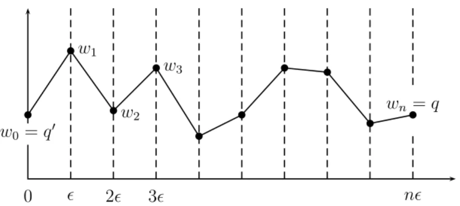
Figure 2.1: A broken path of a particle propagating from w

to w

.

To see more clearly why (2.29) is called a path integral (or functional integral in field theory) we divide the time interval [0, t] into n equidistant intervals with length ǫ = t/n and identify w

with w(s = kǫ), see fig. (2.1). Now we connect every pair of points (jǫ, w

) and (jǫ + ǫ, w

) by a straight line and obtain a broken line path from w

= q

to w

= q

The exponent S

in (2.29) is a Riemann sum approximation to the classical action of a particle moving along this broken line path,

S

(w)

−→

t

Z

0

ds

m

2 w ˙

− V (w)

≡ S[w] (2.30)

The integrations ^R dw

. . . dw

in (2.29) is to be interpreted as summing over all possible broken line paths connecting q

with q. Since any continuous path from q

with q can be ap- proximated by a broken line path and since finally we must take the continuum limit n → ∞ or equivalently ǫ → 0, we may interpret the integral (2.29) as a sum over all paths from q

at time 0 and to q at time t. The ǫ-dependent constant

A

=

m 2πi¯ hǫ

(2.31) in the path integral (2.29) is required to obtain a unitary time evolution. It diverges in the continuum limit ǫ → 0, but this divergence is harmless as we shall see later. In the continuum limit we denote the path integral representation for the evolution kernel (2.29) by

K(t, q, q

) =

w(t)=q

Z

w(0)=q^′

Dw e

, (2.32)

with the formal ’measure’ Dw on the set of paths defined by the limit (2.29). Since the infinite

product of Lebesgue measures like ^Q

dw

fails to be a measure, the symbol Dw is mathemati-

cally not well-defined. However, one can define a measure on the set of paths if one analytically

CHAPTER 2. DERIVING THE PATH INTEGRAL 2.3. Non-stationary systems 14

continues to imaginary time. For more general Lagrangian systems, for example for particles propagating in 3 dimensions, a similar path integral representation for the evolution kernel can be given. In same cases, for example for particle in external fields, ordering ambiguities in the canonical approach translate into discretization ambiguities even in the continuum limit.

2.3 Non-stationary systems

The Feynman-Kac formula not only holds for stationary systems, it also holds for time-dependent Hamiltonians H(t) for which the evolution kernel has the form

K(t, q, t

, q

) = hq| T exp

− i

¯ h

Z

t^′

H(s)ds

|q

i , (2.33)

where T denotes the time ordering. The generalization to time-dependent Hamiltonians is useful when on considers system under varying external conditions, for example in a time-dependent external field. In a non-stationary situation the evolution operator depends on the initial and final times and not only on the time-difference t − t

. But the continuum path integral for the evolution kernel K looks the same as in the stationary case,

K(t, q, t

, q

) =

w(t)=q

Z

w(t^′)=q^′

Dw e

, (2.34)

where now the Lagrange function depends explicitly on time. For a system with Hamiltonian H = H

+ V (t) the path integral is the continuum limit of

K(t, q, t

, q

) = lim

n→∞

A

Z

dw

· · · dw

e

S

(w) = m

2

n−1

X

j=0

w

− w

ǫ

−

n−1

X

j=0

ǫV (t

+ jǫ, w

), (2.35) where ǫ = (t −t

)/n. Note that now the potential depends on the (discretized) time. To establish (2.34) we show that

ψ(t, q) =

Z

K(t, q, t

, q

) ψ(t

, q

) dq

(2.36) obeys the time-dependent Schr¨odinger equation. For that purpose we set t

= t − ǫ with small ǫ. The evolution for a infinitesimal time step ǫ is given by

ψ(t, q) = A

Z

dq

exp

im

2¯ hǫ (q − q

)

− iǫ

¯

h V (t − ǫ, q

)

ψ(t − ǫ, q

).

Changing variables according to q → q

+ u this reads ψ(t, q) = A

Z

du e

e

ψ(t − ǫ, q + u). (2.37)

CHAPTER 2. DERIVING THE PATH INTEGRAL 2.4. Greensfunctions 15

Due to the first Gaussian factor the u-integral gets its main contribution from the neighborhood of u = 0 and thus we may expand the last two factors in powers of u. The resulting integrals over u are computed with the help of the formula

Z

du u

e

= 1 A

i¯ hǫ m

!

(2n − 1)!! (2.38)

where 0!! = (−1)!! = 1 by definition. Of course, the integrals with odd powers of u vanish. We only need the terms of order 1 and ǫ on the right hand side in (2.37) and thus it is sufficient to expand ψ to second order in u. Up to terms of order ǫ

we find

ψ (t, q) = A

Z

du e

1 − iǫ

¯

h V (t, q)

ψ(t − ǫ, q) + u

2 ψ

(t, q)

!

+ O(ǫ

).

The integration over u finally leads to ψ(t, q) = ψ(t − ǫ, q) − iǫ

¯

h V (t, q)ψ(t, q) + i¯ hǫ

m ψ

(t, q) + O(ǫ

). (2.39) Note that for ǫ → 0 the right hand side converges to ψ(t, q) such that K converges to the identity as t

→ t. Now we subtract ψ(t−ǫ, q) from both sides in (2.39) and divide the resulting equation by ǫ. In the continuum limit ǫ → 0 we recover the time-dependent Schr¨odinger equation,

i¯ h ∂ψ

∂t = − ¯ h

2m ψ

+ V (t)ψ, (2.40)

and this shows that even for a time-dependent Hamiltonian the propagator is given by the path integral (2.34) or more accurately by (2.35).

2.4 Greensfunctions

In quantum field theory one is interested in vacuum expectation values of time-ordered products of Heisenberg field operators since these objects are related to amplitudes of physical processes such as scattering amplitudes or decay rates of particles. We look at the analogous objects in quantum mechanics:

G

(t

, t

, . . . , t

) = hΩ| T q(t ˆ

)ˆ q(t

) · · · q(t ˆ

)|Ωi, (2.41) where|Ωi represents the vacuum state and the position operator has the time dependence

ˆ

q(t) = e

qe ˆ

, (2.42) see equation (2.4). The objects G

are known as Greensfunction or correlation functions. The time ordering operator T orders its arguments such that the operator at earliest time acts first (is the right-most), the operator at the second earliest time acts next etc. For example

T q(t ˆ

)ˆ q(t

) =

( q(t ˆ

)ˆ q(t

) t

> t

ˆ

q(t

)ˆ q(t

) t

> t

. (2.43)

CHAPTER 2. DERIVING THE PATH INTEGRAL 2.4. Greensfunctions 16

Now will derive the path integral expression for the Greensfunction (2.41). Actually we shall calculate correlation functions with fixed endpoints, for example

hq, t| T q(t ˆ

)ˆ q(t

)|q

i , where |q, ti = e

|qi (2.44) is the past-evolved position eigenstate, q(t)|t, qi ˆ = q|t, qi. Later we shall see how one recovers the vacuum expectation values (2.41) from the correlation functions with fixed endpoints. We assume t

> t

and insert twice the identity in (2.44), one after every position operator q, ˆ

hq, t| q(t ˆ

)ˆ q(t

)|q

i = hq| e

qe ˆ

qe ˆ

|q

i

=

Z

dw

dw

hq| e

|w

i w

hw

| e

|w

i w

hw

| e

|q

i .

Inserting the path integral representation for the three matrix elements we obtain hq, t| q(t ˆ

)ˆ q(t

)|q

i =

Z

dw

dw

w

w

Z

q(t1)=w1

Dw e

w(t1)=w1

Z

w(t2)=w2

Dw e

w(t2)=w2

Z

q(0)=q^′

Dw e

. (2.45) This expression consists of a first path integral from the initial position q

to the position w

, a second one from w

to the position w

, and a third one from w

to the final position q. So we are integrating over all paths from q

to q, subject to the restriction that the paths pass through the intermediate points w

and w

at times t

and t

, respectively. Finally we integrate over the two arbitrary positions w

and w

, so that in fact we are integrating over all paths. Thus we may combine the three path integrals and the integrations over w

and w

into a single path integral.

The factors w

and w

in the integrand are just the values w(t

) and w(t

) of the paths at the intermediate times. Hence we end up with

hq, t| q(t ˆ

)ˆ q(t

)|q

i =

w(t)=q

Z

w(0)=q^′

Dw w(t

)w(t

) e

(t

> t

). (2.46)

A similar calculation reveals that the same result holds true for the matrix element of q(t ˆ

)ˆ q(t

) when t

> t

. The path integral takes care of the time ordering. Thus we arrive at the following formula for all pairs t

, t

:

hq, t| T q(t ˆ

)ˆ q(t

)|q

i =

w(t)=q

Z

w(0)=q^′

Dw w(t

)w(t

) e

. (2.47)

The generalization to higher correlation function is evident. One obtains hq, t| T q(t ˆ

)ˆ q(t

) · · · q(t ˆ

)|q

i =

w(t)=q

Z

w(0)=q^′

Dw w(t

)w(t

) · · · w(t

) e

. (2.48)

CHAPTER 2. DERIVING THE PATH INTEGRAL 2.4. Greensfunctions 17

Now we relate the time ordered correlation functions for fixed endpoints to the vacuum expecta- tion values in (2.41). Normalizing the Hamiltonian such that its groundstate|Ωi has zero energy, in which case it is time-independent, we obtain

hΩ| =

Z

dq hΩ| q, ti ht, q| =

Z

dq hΩ| qi ht, q| =

Z

dq Ω(q) ¯ ht, q| . (2.49) Now we multiply (2.48) with Ω(q)Ω(q ¯

) and integrate over the arguments q and q

. This yields

hΩ| T q(t ˆ

) · · · q(t ˆ

)|Ωi =

Z

dqdq

Ω(q)Ω(q ¯

)

w(t)=q

Z

w(0)=q^′

Dw w(t

) · · · w(t

) e

. (2.50) Actually, to calculate such vacuum-to-vacuum transition amplitudes one conveniently continues to imaginary time and this will be studied in a later chapter.

Generating functional for time ordered products: The Greenfunctions for time ordered products of position operators at different times are generated by a functional depending on an external source. It is given by the path integral in which a source term is added to the action,

S[w] −→ S

[w] = S[w] + (j, w), (j, w) =

Z

0

dsj(s)w(s). (2.51) The corresponding evolution kernel in the presence of the source

K (t, q, q

; j) =

w(t)=q

Z

w(0)=q^′

Dw e

. (2.52)

is just the generating functional for the Greenfunctions (2.48). For example, its first variational derivative with respect to the source is

¯ h i

δ

δj(t

) K (t, q, q

; j) =

Z

Dw w(t

) e

. (2.53) The n-fold differentiation of K at j = 0 yields the path integral with several w-insertions,

¯ h i

δ

δj(t

) · · · ¯ h i

δ

δj(t

) K(t, q, q

; j )|

=

Z

Dw w(t

) · · · w(t

) e

, (2.54) which according to the result (2.48) is equal to the expectation value of the time-ordered product of n position operators at different times

¯ h i

δ

δj(t

) · · · ¯ h i

δ

δj(t

) K (t, q, q

; j )|

= hq, t| T q(t ˆ

) · · · q(t ˆ

)|q

i . (2.55)

For an interacting system the generating functional cannot be calculated in closed form. But

with the result (2.48) we can easily set up a perturbative expansion for the Greenfunctions. This

will be done in chapter 4.