arXiv:quant-ph/0004090v1 24 Apr 2000
Path Integral Methods and Applications ∗
Richard MacKenzie
†Laboratoire Ren´e-J.-A.-L´evesque Universit´e de Montr´eal Montr´eal, QC H3C 3J7 Canada
UdeM-GPP-TH-00-71
Abstract
These lectures are intended as an introduction to the technique of path integrals and their applications in physics. The audience is mainly first-year graduate students, and it is assumed that the reader has a good foundation in quantum mechanics. No prior exposure to path integrals is assumed, however.
The path integral is a formulation of quantum mechanics equivalent to the standard formulations, offering a new way of looking at the subject which is, arguably, more intuitive than the usual approaches. Applications of path integrals are as vast as those of quantum mechanics itself, including the quantum mechanics of a single particle, statistical mechanics, condensed matter physics and quantum field theory.
After an introduction including a very brief historical overview of the subject, we derive a path integral expression for the propagator in quantum mechanics, including the free particle and harmonic oscillator as examples. We then discuss a variety of applications, including path integrals in multiply-connected spaces, Euclidean path integrals and statistical mechanics, perturbation theory in quantum mechanics and in quantum field theory, and instantons via path integrals.
For the most part, the emphasis is on explicit calculations in the familiar setting of quantum mechanics, with some discussion (often brief and schematic) of how these ideas can be applied to more complicated situations such as field theory.
∗Lectures given at Rencontres du Vietnam: VIth Vietnam School of Physics, Vung Tau, Vietnam, 27 December 1999 - 8 January 2000.
†rbmack@lps.umontreal.ca
1
1 Introduction
1.1 Historical remarks
We are all familiar with the standard formulations of quantum mechanics, developed more or less concurrently by Schroedinger, Heisenberg and others in the 1920s, and shown to be equivalent to one another soon thereafter.
In 1933, Dirac made the observation that the action plays a central role in classical mechanics (he considered the Lagrangian formulation of classical mechanics to be more fundamental than the Hamiltonian one), but that it seemed to have no important role in quantum mechanics as it was known at the time. He speculated on how this situation might be rectified, and he arrived at the conclusion that (in more modern language) the propagator in quantum mechanics “corresponds to” expiS/¯h, where S is the classical action evaluated along the classical path.
In 1948, Feynman developed Dirac’s suggestion, and succeeded in deriving a third formu- lation of quantum mechanics, based on the fact that the propagator can be written as a sum over all possible paths (not just the classical one) between the initial and final points. Each path contributes expiS/¯h to the propagator. So while Dirac considered only the classical path, Feynman showed that all paths contribute: in a sense, the quantum particle takes all paths, and the amplitudes for each path add according to the usual quantum mechanical rule for combining amplitudes. Feynman’s original paper,1 which essentially laid the foundation of the subject (and which was rejected by Physical Review!), is an all-time classic, and is highly recommended. (Dirac’s original article is not bad, either.)
1.2 Motivation
What do we learn from path integrals? As far as I am aware, path integrals give us no dramatic new results in the quantum mechanics of a single particle. Indeed, most if not all calculations in quantum mechaincs which can be done by path integrals can be done with considerably greater ease using the standard formulations of quantum mechanics. (It is probably for this reason that path integrals are often left out of undergraduate-level quantum mechanics courses.) So why the fuss?
As I will mention shortly, path integrals turn out to be considerably more useful in more complicated situations, such as field theory. But even if this were not the case, I believe that path integrals would be a very worthwhile contribution to our understanding of quantum mechanics. Firstly, they provide a physically extremely appealing and intuitive way of viewing quantum mechanics: anyone who can understand Young’s double slit experiment in optics should be able to understand the underlying ideas behind path integrals. Secondly, the classical limit of quantum mechanics can be understood in a particularly clean way via path integrals.
It is in quantum field theory, both relativistic and nonrelativistic, that path integrals (functional integrals is a more accurate term) play a much more important role, for several
1References are not cited in the text, but a short list of books and articles which I have found interesting and useful is given at the end of this article.
1 INTRODUCTION 3 reasons. They provide a relatively easy road to quantization and to expressions for Green’s functions, which are closely related to amplitudes for physical processes such as scattering and decays of particles. The path integral treatment of gauge field theories (non-abelian ones, in particular) is very elegant: gauge fixing and ghosts appear quite effortlessly. Also, there are a whole host of nonperturbative phenomena such as solitons and instantons that are most easily viewed via path integrals. Furthermore, the close relation between statistical mechanics and quantum mechanics, or statistical field theory and quantum field theory, is plainly visible via path integrals.
In these lectures, I will not have time to go into great detail into the many useful ap- plications of path integrals in quantum field theory. Rather than attempting to discuss a wide variety of applications in field theory and condensed matter physics, and in so doing having to skimp on the ABCs of the subject, I have chosen to spend perhaps more time and effort than absolutely necessary showing path integrals in action (pardon the pun) in quantum mechanics. The main emphasis will be on quantum mechanical problems which are not necessarily interesting and useful in and of themselves, but whose principal value is that they resemble the calculation of similar objects in the more complex setting of quantum field theory, where explicit calculations would be much harder. Thus I hope to illustrate the main points, and some technical complications and hangups which arise, in relatively famil- iar situations that should be regarded as toy models analogous to some interesting contexts in field theory.
1.3 Outline
The outline of the lectures is as follows. In the next section I will begin with an introduction to path integrals in quantum mechanics, including some explicit examples such as the free particle and the harmonic oscillator. In Section 3, I will give a “derivation” of classical mechanics from quantum mechanics. In Section 4, I will discuss some applications of path integrals that are perhaps not so well-known, but nonetheless very amusing, namely, the case where the configuration space is not simply connected. (In spite of the fancy terminology, no prior knowledge of high-powered mathematics such as topology is assumed.) Specifi- cally, I will apply the method to the Aharonov-Bohm effect, quantum statistics and anyons, and monopoles and charge quantization, where path integrals provide a beautifully intuitive approach. In Section 5, I will explain how one can approach statistical mechanics via path in- tegrals. Next, I will discuss perturbation theory in quantum mechanics, where the technique used is (to put it mildly) rather cumbersome, but nonetheless illustrative for applications in the remaining sections. In Section 7, I will discuss Green’s functions (vacuum expectation values of time-ordered products) in quantum mechanics (where, to my knowledge, they are not particularly useful), and will construct the generating functional for these objects. This groundwork will be put to good use in the following section, where the generating functional for Green’s functions in field theory (which are useful!) will be elucidated. In Section 9, I will discuss instantons in quantum mechanics, and will at least pay lip service to important applications in field theory. I will finish with a summary and a list of embarrassing omissions.
1 INTRODUCTION 4 I will conclude with a few apologies. First, an educated reader might get the impression that the outline given above contains for the most part standard material. S/he is likely correct: the only original content to these lectures is the errors.2
Second, I have made no great effort to give complete references (I know my limitations);
at the end of this article I have listed some papers and books from which I have learned the subject. Some are books or articles wholly devoted to path integrals; the majority are books for which path integrals form only a small (but interesting!) part. The list is hopelessly incomplete; in particular, virtually any quantum field theory book from the last decade or so has a discussion of path integrals in it.
Third, the subject of path integrals can be a rather delicate one for the mathematical purist. I am not one, and I have neither the interest nor the expertise to go into detail about whether or not the path integral exists, in a strict sense. My approach is rather pragmatic:
it works, so let’s use it!
2Even this joke is borrowed from somewhere, though I can’t think of where.
2 Path Integrals in Quantum Mechanics
2.1 General discussion
Consider a particle moving in one dimension, the Hamiltonian being of the usual form:
H = p2
2m +V(q).
The fundamental question in the path integral (PI) formulation of quantum mechanics is:
If the particle is at a position q at timet = 0, what is the probability amplitude that it will be at some other position q′ at a later time t=T?
It is easy to get a formal expression for this amplitude in the usual Schroedinger formu- lation of quantum mechanics. Let us introduce the eigenstates of the position operator ˆq, which form a complete, orthonormal set:
ˆ
q|qi=q|qi, hq′|qi=δ(q′−q),
Z
dq|qi hq|= 1.
(When there is the possibility of an ambiguity, operators will be written with a “hat”;
otherwise the hat will be dropped.) Then the initial state is |ψ(0)i=|qi. Letting the state evolve in time and projecting on the state |q′i, we get for the amplitude A,
A=hq′|ψ(T)i ≡K(q′, T;q,0) =hq′|e−iHT |qi. (1) (Except where noted otherwise, ¯hwill be set to 1.) This object, for obvious reasons, is known as the propagator from the initial spacetime point (q,0) to the final point (q′, T). Clearly, the propagator is independent of the origin of time: K(q′, T +t;q, t) =K(q′, T;q,0).
We will derive an expression for this amplitude in the form of a summation (integral, really) over all possible paths between the initial and final points. In so doing, we derive the PI from quantum mechanics. Historically, Feynman came up with the PI differently, and showed its equivalence to the usual formulations of quantum mechanics.
Let us separate the time evolution in the above amplitude into two smaller time evolu- tions, writing e−iHT =e−iH(T−t1)e−iHt1. The amplitude becomes
A=hq′|e−iH(T−t1)e−iHt1|qi.
Inserting a factor 1 in the form of a sum over the position eigenstates gives A = hq′|e−iH(T−t1)
Z
dq1|q1i hq1|
| {z }
=1
e−iHt1|qi
=
Z
dq1K(q′, T;q1, t1)K(q1, t1;q,0). (2) This formula is none other than an expression of the quantum mechanical rule for combining amplitudes: if a process can occur a number of ways, the amplitudes for each of these ways add. A particle, in propagating from q toq′, must besomewhere at an intermediate timet1; labelling that intermediate position q1, we compute the amplitude for propagation via the
2 PATH INTEGRALS IN QUANTUM MECHANICS 6 point q1 [this is the product of the two propagators in (2)] and integrate over all possible intermediate positions. This result is reminiscent of Young’s double slit experiment, where the amplitudes for passing through each of the two slits combine and interfere. We will look at the double-slit experiment in more detail when we discuss the Aharonov-Bohm effect in Section 4.
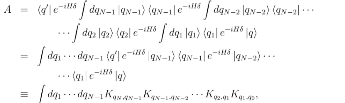
We can repeat the division of the time interval T; let us divide it up into a large number N of time intervals of durationδ =T /N. Then we can write for the propagator
A =hq′|e−iHδN|qi=hq′|e−iHδe−iHδ· · ·e−iHδ
| {z }
N times
|qi.
We can again insert a complete set of states between each exponential, yielding A = hq′|e−iHδ
Z
dqN−1|qN−1i hqN−1|e−iHδ
Z
dqN−2|qN−2i hqN−2| · · ·
· · ·
Z
dq2|q2i hq2|e−iHδ
Z
dq1|q1i hq1|e−iHδ|qi
=
Z
dq1· · ·dqN−1hq′|e−iHδ|qN−1i hqN−1|e−iHδ|qN−2i · · ·
· · · hq1|e−iHδ|qi
≡
Z
dq1· · ·dqN−1KqN,qN−1KqN−1,qN−2· · ·Kq2,q1Kq1,q0, (3) where we have defined q0 =q, qN = q′. (Note that these initial and final positions are not integrated over.) This expression says that the amplitude is the integral of the amplitude of allN-legged paths, as illustrated in Figure 1.
3 q2
qN-2 qN-1
q1
δ (N-1) q
. . . .
t δ 2δ 3δ T
q’=q
q=q0
N
q
Figure 1: Amplitude as a sum over all N-legged paths.
Apart from mathematical details concerning the limit when N → ∞, this is clearly going to become a sum over all possible paths of the amplitude for each path:
A= X
paths
Apath,
where
X
paths
=
Z
dq1· · ·dqN−1, Apath =KqN,qN−1KqN−1,qN−2· · ·Kq2,q1Kq1,q0.
2 PATH INTEGRALS IN QUANTUM MECHANICS 7 Let us look at this last expression in detail.
The propagator for one sub-interval is Kqj+1,qj = hqj+1|e−iHδ|qji. We can expand the exponential, since δ is small:
Kqj+1,qj = hqj+1|
1−iHδ− 1
2H2δ2+· · ·
|qji
= hqj+1|qji −iδhqj+1|H|qji+o(δ2). (4) The first term is a delta function, which we can write3
hqj+1|qji=δ(qj+1−qj) =
Z dpj
2πeipj(qj+1−qj). (5) In the second term of (4), we can insert a factor 1 in the form of an integral over momentum eigenstates between H and |qji; this gives
−iδhqj+1| pˆ2
2m +V(ˆq)
! Z dpj
2π |pji hpj|qji
=−iδ
Z dpj
2π pj2
2m +V(qj+1)
!
hqj+1|pji hpj|qji
=−iδ
Z dpj
2π pj2
2m +V(qj+1)
!
eipj(qj+1−qj), (6) using hq|pi = expipq. In the first line, we view the operator ˆp as operating to the right, while V(ˆq) operates to the left.
The expression (6) is asymmetric between qj and qj+1; the origin of this is our choice of putting the factor 1 to the right of H in the second term of (4). Had we put it to the left instead, we would have obtainedV(qj) in (6). To not play favourites, we should choose some sort of average of these two. In what follows I will simply writeV(¯qj) where ¯qj = 12(qj+qj+1).
(The exact choice does not matter in the continuum limit, which we will take eventually;
the above is a common choice.) Combining (5) and (6), the sub-interval propagator is Kqj+1,qj =
Z dpj
2πeipj(qj+1−qj) 1−iδ pj2
2m +V(¯qj)
!
+o(δ2)
!
=
Z dpj
2πeipj(qj+1−qj)e−iδH(pj,¯qj)(1 +o(δ2)). (7) There areN such factors in the amplitude. Combining them, and writing ˙qj = (qj+1−qj)/δ, we get
Apath =
Z N−1Y
j=0
dpj
2π expiδ
N−1X
j=0
(pjq˙j −H(pj,q¯j)), (8) where we have neglected a multiplicative factor of the form (1 +o(δ2))N, which will tend toward one in the continuum limit. Then the propagator becomes
K =
Z
dq1· · ·dqN−1Apath
=
Z N−1
Y
j=1
dqj
Z N−1
Y
j=0
dpj
2π expiδ
N−1
X
j=0
(pjq˙j−H(pj,q¯j)). (9)
3Please do not confuse the delta function with the time interval,δ.
2 PATH INTEGRALS IN QUANTUM MECHANICS 8 Note that there is one momentum integral for each interval (N total), while there is one position integral for each intermediate position (N −1 total).
If N → ∞, this approximates an integral over all functions p(t), q(t). We adopt the following notation:
K ≡
Z
Dp(t)Dq(t) expi
Z T
0 dt(pq˙−H(p, q)). (10) This result is known as the phase-space path integral. The integral is viewed as over all functionsp(t) and over all functionsq(t) whereq(0) =q,q(T) = q′. But to actually perform an explicit calculation, (10) should be viewed as a shorthand notation for the more ponderous expression (9), in the limit N → ∞.
If, as is often the case (and as we have assumed in deriving the above expression), the Hamiltonian is of the standard form, namelyH =p2/2m+V(q), we can actually carry out the momentum integrals in (9). We can rewrite this expression as
K =
Z N−1Y
j=1
dqjexp−iδ
N−1X
j=0
V(¯qj)
Z N−1Y
j=0
dpj
2π expiδ
N−1X
j=0
pjq˙j −pj2/2m. The p integrals are all Gaussian, and they are uncoupled. One such integral is
Z dp
2πeiδ(pq−p˙ 2/2m) =
r m
2πiδeiδmq˙2/2.
(The careful reader may be worried about the convergence of this integral; if so, a factor exp−ǫp2 can be introduced and the limit ǫ→0 taken at the end.)
The propagator becomes
K =
Z N−1
Y
j=1
dqjexp−iδ
N−1X
j=0
V(¯qj)
N−1
Y
j=0
r m
2πiδ expiδmq˙j2 2
!
=
m 2πiδ
N/2Z N−1
Y
j=1
dqjexpiδ
N−1X
j=0
mq˙j2
2 −V(¯qj)
!
. (11)
The argument of the exponential is a discrete approximation of the action of a path passing through the points q0 = q, q1,· · ·, qN−1, qN = q′. As above, we can write this in the more compact form
K =
Z
Dq(t)eiS[q(t)]. (12)
This is our final result, and is known as the configuration space path integral. Again, (12) should be viewed as a notation for the more precise expression (11), as N → ∞.
2.2 Examples
To solidify the notions above, let us consider a few explicit examples. As a first example, we will compute the free particle propagator first using ordinary quantum mechanics and then via the PI. We will then mention some generalizations which can be done in a similar manner.
2 PATH INTEGRALS IN QUANTUM MECHANICS 9 2.2.1 Free particle
Let us compute the propagatorK(q′, T;q,0) for a free particle, described by the Hamiltonian H = p2/2m. The propagator can be computed straightforwardly using ordinary quantum mechanics. To this end, we write
K = hq′|e−iHT |qi
= hq′|e−iTpˆ2/2m
Z dp
2π|pi hp|qi
=
Z dp
2πe−iT p2/2mhq′|pi hp|qi
=
Z dp
2πe−iT(p2/2m)+i(q′−q)p. (13)
The integral is Gaussian; we obtain K =
m 2πiT
1/2
eim(q′−q)2/2T. (14) Let us now see how the same result can be attained using PIs. The configuration space PI (12) is
K = lim
N→∞
m 2πiδ
N/2Z N−1Y
j=1
dqj expimδ 2
N−1X
j=0
qj+1−qj δ
2
= lim
N→∞
m 2πiδ
N/2Z N−1
Y
j=1
dqj expim 2δ
h(qN −qN−1)2+ (qN−1−qN−2)2+· · · +(q2−q1)2+ (q1−q0)2i,
where q0 = q and qN = q′ are the initial and final points. The integrals are Gaussian, and can be evaluated exactly, although the fact that they are coupled complicates matters significantly. The result is
K = lim
N→∞
m 2πiδ
N/2 1
√N
2πiδ m
!(N−1)/2
eim(q′−q)2/2N δ
= lim
N→∞
m 2πiNδ
1/2
eim(q′−q)2/2N δ.
But Nδ is the total time interval T, resulting in K =
m 2πiT
1/2
eim(q′−q)2/2T,
in agreement with (14).
A couple of remarks are in order. First, we can write the argument of the exponential as T · 12m((q′−q)/T)2, which is just the action S[qc] for a particle moving along the classical path (a straight line in this case) between the initial and final points.
2 PATH INTEGRALS IN QUANTUM MECHANICS 10 Secondly, we can restore the factors of ¯h if we want, by ensuring correct dimensions. The argument of the exponential is the action, so in order to make it a pure number we must divide by ¯h; furthermore, the propagator has the dimension of the inner product of two position eigenstates, which is inverse length; in order that the coefficient have this dimension we must multiply by ¯h−1/2. The final result is
K =
m 2πi¯hT
1/2
eiS[qc]/¯h. (15)
This result typifies a couple of important features of calculations in this subject, which we will see repeatedly in these lectures. First, the propagator separates into two factors, one of which is the phase expiS[qc]/¯h. Second, calculations in the PI formalism are typically quite a bit more lengthy than using standard techniques of quantum mechanics.
2.2.2 Harmonic oscillator
As a second example of the computation of a PI, let us compute the propagator for the harmonic oscillator using this method. (In fact, we will not do the entire computation, but we will do enough to illustrate a trick or two which will be useful later on.)
Let us start with the somewhat-formal version of the configuration-space PI, (12):
K(q′, T;q,0) =
Z
Dq(t)eiS[q(t)]. For the harmonic oscillator,
S[q(t)] =
Z T
0 dt
1
2mq˙2−1
2mω2q2
.
The paths over which the integral is to be performed go from q(0) = q to q(T) =q′. To do this PI, suppose we know the solution of the classical problem, qc(t):
¨
qc +ω2qc = 0, qc(0) =q, qc(T) =q′.
We can write q(t) = qc(t) + y(t), and perform a change of variables in the PI to y(t), since integrating over all deviations from the classical path is equivalent to integrating over all possible paths. Since at each time q and y differ by a constant, the Jacobian of the transformation is 1. Furthermore, since qc obeys the correct boundary conditions, the paths y(t) over which we integrate go fromy(0) = 0 toy(T) = 0. The action for the pathqc(t)+y(t) can be written as a power series in y:
S[qc(t) +y(t)] =
Z T
0 dt
1
2mq˙c2− 1
2mω2qc2
+ (linear in y)
| {z }
=0
+
Z T
0 dt
1
2my˙2− 1
2mω2y2
.
The term linear in y vanishes by construction: qc, being the classical path, is that path for which the action is stationary! So we may write S[qc(t) +y(t)] = S[qc(t)] +S[y(t)]. We substitute this into (12), yielding
K(q′, T;q,0) =eiS[qc(t)]
Z
Dy(t)eiS[y(t)]. (16)
2 PATH INTEGRALS IN QUANTUM MECHANICS 11 As mentioned above, the paths y(t) over which we integrate go from y(0) = 0 to y(T) = 0:
the only appearance of the initial and final positions is in the classical path, i.e., in the classical action. Once again, the PI separates into two factors. The first is written in terms of the action of the classical path, and the second is a PI over deviations from this classical path. The second factor is independent of the initial and final points.
This separation into a factor depending on the action of the classical path and a second one, a PI which is independent of the details of the classical path, is a recurring theme, and an important one. Indeed, it is often the first factor which contains most of the useful information contained in the propagator, and it can be deduced without even performing a PI. It can be said that much of the work in the game of path integrals consists in avoiding having to actually compute one!
As for the evaluation of (16), a number of fairly standard techniques are available. One can calculate the PI directly in position space, as was done above for the harmonic oscillator (see Schulman, chap. 6). Alternatively, one can compute it in Fourier space (writing y(t) =
P
kaksin(kπt/T) and integrating over the coefficients{ak}). This latter approach is outlined in Feynman and Hibbs, Section 3.11. The result is
K(q′, T;q,0) =
mω 2πisinωT
1/2
eiS[qc(t)]. (17) The classical action can be evaluated straightforwardly (note that this is not a PI problem, nor even a quantum mechanics problem!); the result is
S[qc(t)] = mω 2 sinωT
(q′2+q2) cosωT −2q′q.
We close this section with two remarks. First, the PI for any quadratic action can be evaluated exactly, essentially since such a PI consists of Gaussian integrals; the general result is given in Schulman, Chapter 6. In Section 6, we will evaluate (to the same degree of completeness as the harmonic oscillator above) the PI for a forced harmonic oscillator, which will prove to be a very useful tool for computing a variety of quantities of physical interest.
Second, the following fact is not difficult to prove, and will be used below (Section 4.2.).
K(q′, T;q,0) (whether computed via PIs or not) is the amplitude to propagate from one point to another in a given time interval. But this is the response to the following question:
If a particle is initially at positionq, what is its wave function after the elapse of a time T? Thus, if we consider K as a function of the final position and time, it is none other than the wave function for a particle with a specific initial condition. As such, the propagator satisfies the Schroedinger equation at its final point.
3 The Classical Limit: “Derivation” of the Principle of Least Action
Since the example calculations performed above are somewhat dry and mathematical, it is worth backing up a bit and staring at the expression for the configuration space PI, (12):
K =
Z
Dq(t)eiS[q(t)]/¯h.
This innocent-looking expression tells us something which is at first glance unbelievable, and at second glancereally unbelievable. The first-glance observation is that a particle, in going from one position to another, takes all possible paths between these two positions. This is, if not actually unbelievable, at the very least least counter-intuitive, but we could argue away much of what makes us feel uneasy if we could convince ourselves that while all paths contribute, the classical path is the dominant one.
However, the second-glance observation is not reassuring: if we compare the contribution of the classical path (whose action is S[qc]) with that of some other, arbitrarily wild, path (whose action is S[qw]), we find that the first is expiS[qc] while the second is expiS[qw].
They are both complex numbers of unit magnitude: each path taken in isolation is equally important. The classical path is no more important than any arbitrarily complicated path!
How are we to reconcile thisreallyunbelievable conclusion with the fact that a ball thrown in the air has a more-or-less parabolic motion?
The key, not surprisingly, is in how different paths interfere with one another, and by considering the case where the rough scale of classical action of the problem is much bigger than the quantum of action, ¯h, we will see the emergence of the Principle of Least Action.
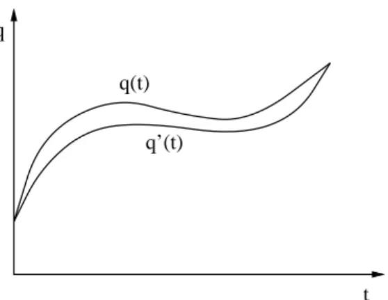
Consider two neighbouring paths q(t) and q′(t) which contribute to the PI (Figure 2).
Letq′(t) =q(t) +η(t), with η(t) small. Then we can write the action as a functional Taylor expansion about the classical path:4
S[q′] =S[q+η] =S[q] +
Z
dt η(t)δS[q]
δq(t) +o(η2).
The two paths contribute expiS[q]/¯h and expiS[q′]/¯hto the PI; the combined contribution is
A≃eiS[q]/¯h 1 + exp i
¯ h
Z
dt η(t)δS[q]
δq(t)
!
,
where we have neglected corrections of order η2. We see that the difference in phase be- tween the two paths, which determines the interference between the two contributions, is
¯
h−1R dt η(t)δS[q]/δq(t).
We see that the smaller the value of ¯h, the larger the phase difference between two given paths. So even if the paths are very close together, so that the difference in actions is extremely small, for sufficiently small ¯h the phase difference will still be large, and on average destructive interference occurs.
4The reader unfamiliar with manipulation of functionals need not despair; the only rule needed beyond standard calculus is the functional derivative: δq(t)/δq(t′) = δ(t−t′), where the last δ is the Dirac delta function.
3 CLASSICAL LIMIT 13
t q’(t)
q
q(t)
Figure 2: Two neighbouring paths.
However, this argument must be rethought for one exceptional path: that which extrem- izes the action, i.e., the classical path, qc(t). For this path, S[qc+η] = S[qc] +o(η2). Thus the classical path and a very close neighbour will have actions which differ by much less than two randomly-chosen but equally close paths (Figure 3). This means that for fixed closeness
cl paths interfere
constructively
paths interfere destructively
q
t q
Figure 3: Paths near the classical path interfere constructively.
of two paths (I leave it as an exercise to make this precise!) and for fixed ¯h, paths near the classical path will on average interfere constructively (small phase difference) whereas for random paths the interference will be on average destructive.
Thus heuristically, we conclude that if the problem is classical (action ≫ ¯h), the most important contribution to the PI comes from the region around the path which extremizes the PI. In other words, the particle’s motion is governed by the principle that the action is stationary. This, of course, is none other than the Principle of Least Action from which the Euler-Lagrange equations of classical mechanics are derived.
4 Topology and Path Integrals in Quantum Mechanics:
Three Applications
In path integrals, if the configuration space has holes in it such that two paths between the same initial and final point are not necessarily deformable into one another, interesting effects can arise. This property of the configuration space goes by the following catchy name:
non-simply-connectedness. We will study three such situations: the Aharonov-Bohm effect, particle statistics, and magnetic monopoles and the quantization of electric charge.
4.1 Aharonov-Bohm effect
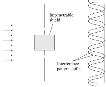
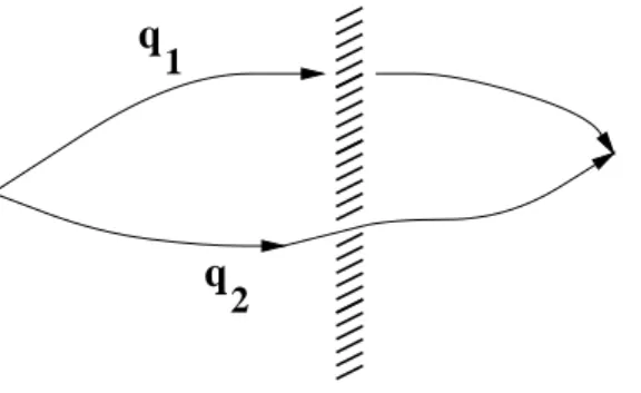
The Aharonov-Bohm effect is one of the most dramatic illustrations of a purely quantum effect: the influence of the electromagnetic potential on particle motion even if the particle is perfectly shielded from any electric or magnetic fields. While classically the effect of electric and magnetic fields can be understood purely in terms of the forces these fields create on particles, Aharonov and Bohm devised an ingenious thought-experiment (which has since been realized in the laboratory) showing that this is no longer true in quantum mechanics.
Their effect is best illustrated by a refinement of Young’s double-slit experiment, where particles passing through a barrier with two slits in it produce an interference pattern on a screen further downstream. Aharonov and Bohm proposed such an experiment performed with charged particles, with an added twist provided by a magnetic flux from which the particles are perfectly shielded passing between the two slits. If we perform the experiment
Impenetrable shield
Interference pattern shifts
Φ
Figure 4: Aharonov-Bohm effect. Magnetic flux is confined within the shaded area; particles are excluded from this area by a perfect shield.
first with no magnetic flux and then with a nonzero and arbitrary flux passing through the shielded region, the interference pattern will change, in spite of the fact that the particles are perfectly shielded from the magnetic field and feel no electric or magnetic force whatsoever.
4 TOPOLOGY AND PATH INTEGRALS 15 Classically we can say: no force, no effect. Not so in quantum mechanics. PIs provide a very attractive way of understanding this effect.
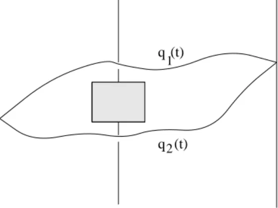
Consider first two representative paths q1(t) and q2(t) (in two dimensions) passing through slits 1 and 2, respectively, and which arrive at the same spot on the screen (Figure 5). Before turning on the magnetic field, let us suppose that the actions for these paths are S[q1] and S[q2]. Then the interference of the amplitudes is determined by
eiS[q1]/¯h+eiS[q2]/¯h =eiS[q1]/¯h1 +ei(S[q2]−S[q1])/¯h.
The relative phase is φ12≡(S[q2]−S[q1])/¯h. Thus these two paths interfere constructively if φ12 = 2nπ, destructively if φ12 = (2n+ 1)π, and in general there is partial cancellation between the two contributions.
2(t) q1(t)
q
Figure 5: Two representative paths contributing to the amplitude for a given point on the screen.
How is this result affected if we add a magnetic field, B? We can describe this field by a vector potential, writing B = ∇ ×A. This affects the particle’s motion by the following change in the Lagrangian:
L( ˙q,q)→L′( ˙q,q) =L( ˙q,q)− e
cv·A(q).
Thus the action changes by
−e c
Z
dtv·A(q) =−e c
Z
dtdq(t)
dt ·A(q(t)).
This integral is R dq·A(q), the line integral ofA along the path taken by the particle. So including the effect of the magnetic field, the action of the first path is
S′[q1] = S[q1]− e c
Z
q1(t)dq·A(q), and similarly for the second path.
Let us now look at the interference between the two paths, including the magnetic field.
eiS′[q1]/¯h+eiS′[q2]/¯h = eiS′[q1]/¯h1 +ei(S′[q2]−S′[q1])/¯h
= eiS′[q1]/¯h1 +eiφ′12, (18)
4 TOPOLOGY AND PATH INTEGRALS 16
where the new relative phase is φ′12 =φ12− e
¯ hc
Z
q2(t)dq·A(q)−
Z
q1(t)dq·A(q)
!
. (19)
But the difference in line integrals in (19) is a contour integral:
Z
q2(t)dq·A(q)−
Z
q1(t)dq·A(q) =
I
dq·A(q) = Φ,
Φ being the flux inside the closed loop bounded by the two paths. So we can write φ′12 =φ12− eΦ
¯ hc.
It is important to note that the change of relative phase due to the magnetic field is independent of the details of the two paths, as long as each passes through the corresponding slit. This means that the PI expression for the amplitude for the particle to reach a given point on the screen is affected by the magnetic field in a particularly clean way. Before the magnetic field is turned on, we may writeA =A1+A2, where
A1 =
Z
slit 1DqeiS[q]/¯h, and similarly for A2. Including the magnetic field,
A′1 =
Z
slit 1Dqei(S[q]−(e/c)R
dq·A)/¯h =e−ieR1dq·A/¯hcA1,
where we have pulled the line integral out of the PI since it is the same for all paths passing through slit 1 arriving at the point on the screen under consideration. So the amplitude is
A = e−ieR1dq·A/¯hcA1+e−ieR2dq·A/¯hcA2
= e−ieR1dq·A/¯hcA1+e−ieHdq·A/¯hcA2
= e−ieR1dq·A/¯hcA1+e−ieΦ/¯hcA2
.
The overall phase is irrelevant, and the interference pattern is influenced directly by the phase eΦ/¯hc. If we vary this phase continuously (by varying the magnetic flux), we can detect a shift in the interference pattern. For example, if eΦ/¯hc = π, then a spot on the screen which formerly corresponded to constructive interference will now be destructive, and vice-versa.
Since the interference is dependent only on the phase difference mod 2π, as we vary the flux we get a shift of the interference pattern which is periodic, repeating itself when eΦ/¯hc changes by an integer times 2π.
4 TOPOLOGY AND PATH INTEGRALS 17
4.2 Particle Statistics
The path integral can be used to see that particles in three dimensions must obey either Fermi or Bose statistics, whereas particles in two dimensions can have intermediate (or fractional) statistics. Consider a system of two identical particles; suppose that there is a short range, infinitely strong repulsive force between the two. We might ask the following question: if at t = 0 the particles are at q1 and q2, what is the amplitude that the particles will be at q′1 and q′2 at some later time T? We will first examine this question in three dimensions, and then in two dimensions.
4.2.1 Three dimensions
According to the PI description of the problem, this amplitude is A= X
paths
eiS[q1(t),q2(t)],
where we sum over all two-particle paths going fromq1,q2 toq′1,q′2.
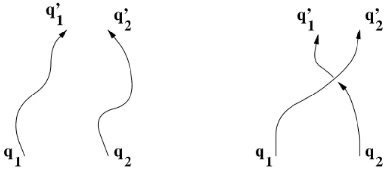
However there is an important subtlety at play: if the particles are identical, then there are (in three dimensions!) two classes of paths (Figure 6).
1 q
2
q’1 q’
2
q1
q q
2
q’1 q’
2
Figure 6: Two classes of paths.
Even though the second path involves an exchange of particles, the final configuration is the same due to the indistinguishability of the particles.
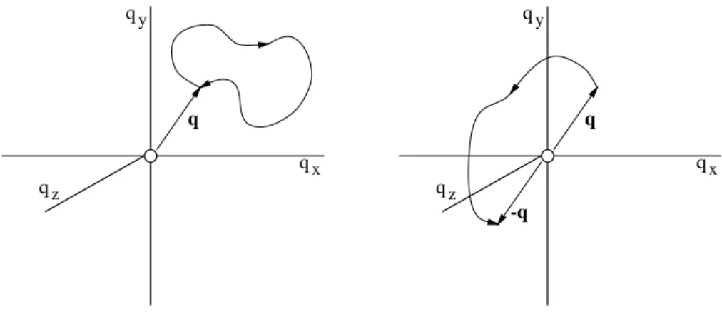
It is more economical to describe this situation in terms of the centre-of-mass position Q= (q1+q2)/2 and the relative positionq=q2−q1. The movement of the centre of mass is irrelevant, and we can concentrate on the relative coordinate q. We can also assume for simplicity that the final positions are the same as the initial ones. Then the two paths above correspond to the paths in relative position space depicted in Figure 7.
The point is, of course, that the relative positions qand −qrepresent the same configu- ration: interchanging q1 and q2 changes q→ −q.
We can elevate somewhat the tone of the discussion by introducing some amount of formalism. The configuration space for the relative position of two identical particles is not R3−{0},5 as one would have naively thought, but (R3−{0})/Z2. The division by the factor
5Recall that we have supposed that the particles have an infinite, short-range repulsion; hence the sub- traction of the origin (which represents coincident points).
4 TOPOLOGY AND PATH INTEGRALS 18 Z2 indicates that opposite points in the space R3− {0}, namely any point qand the point diametrically opposite to it −q, are to be identified: they represent the same configuration.
We must keep this in mind when we attempt to draw paths: the second path of Figure 7 is a closedone.
A topological space such as our configuration space can be characterized as simply con- nected or as non-simply connected according to whether all paths starting and finishing at the same point can or cannot be contracted into the trivial path (representing no relative motion of the particles). It is clear from Figure 7 that the first path can be deformed to the trivial path, while the second one cannot, so the configuration space is not simply connected.
Clearly any path which does not correspond to an exchange of the particles (a “direct” path) is topologically trivial, while any “exchange” path is not; we can divide the space of paths on the configuration space into two topological classes (direct and exchange).
Our configuration space is more precisely described as doubly-connected, since any two topologically nontrivial (exchange) paths taken one after the other result in a direct path, which is trivial. Thus the classes of paths form the elements of the group Z2 if we define the product of two paths to mean first one path followed by the other (a definition which extends readily to the product of classes).
One final bit of mathematical nomenclature: our configuration space, as noted above, is (R3− {0})/Z2, which is not simply connected. We define the (simply connected) covering spaceas the simply connected space which looks locally like the original space. In our case, the covering space is just R3− {0}.
At this point you might well be wondering: what does this have to do with PIs? We can rewrite the PI expression for the amplitude as the following PI in the covering space R3− {0}:
A(q, T;q,0) = X
direct
eiS[q]+ X
exchange
eiS[q]
= A(q, T¯ ;q,0) + ¯A(−q, T;q,0). (20) The notation ¯A is used to indicate that these PIs are in the covering space, while A is a PI in the configuration space. The first term is the sum over all paths from qto q; the second is that for paths from qto −q.
qx qy
qz
-q
qx qy
qz
q q
Figure 7: Paths in relative coordinate space.
4 TOPOLOGY AND PATH INTEGRALS 19 Notice that each sub-path integral is a perfectly respectable PI in its own right: each would be a complete PI for the same dynamical problem but involving distinguishable parti- cles. Since the PI can be thought of as a technique for obtaining the propagator in quantum mechanics, and since (as was mentioned at the end of Section 2) the propagator is a solution of the Schroedinger equation, either of these sub-path integrals also satisfies it. It follows that we can generalize the amplitude A to the following expression, which still satisfies the Schroedinger equation:
A(q, T;q,0)→Aφ(q, T;q,0) = X
direct
eiS[q]+eiφ X
exchange
eiS[q]
= A(q, T¯ ;q,0) +eiφA(¯ −q, T;q,0). (21) This generalization might appear to bead hocand ill-motivated, but we will see shortly that it is intimately related to particle statistics.
There is a restriction on the added phase,φ. To see this, suppose that we no longer insist that the path be a closed one fromq toq. Then (21) generalizes to
Aφ(q′, T;q,0) = ¯A(q′, T;q,0) +eiφA(¯ −q′, T;q,0). (22) If we varyq′ continuously to the point −q′, we have
Aφ(−q′, T;q,0) = ¯A(−q′, T;q,0) +eiφA(q¯ ′, T;q,0). (23) But since the particles are identical, the new final configuration −q′ is identical to old one q′. (22) and (23) are expressions for the amplitude for the same physical process, and can differ at most by a phase:
Aφ(q′, T;q,0) =eiαAφ(−q′, T;q,0).
Combining these three equations, we see that
A(q¯ ′, T;q,0) +eiφA(¯ −q′, T;q,0) =eiαA(¯ −q′, T;q,0) +eiφA(q¯ ′, T;q,0). Equating coefficients of the two terms, we have α=φ (up to a 2π ambiguity), and
ei2φ = 1.
This equation has two physically distinct solutions: φ = 0 and φ =π. (Adding 2nπ results in physically equivalent solutions.)
If φ= 0, we obtain
A(q, T;q,0) = ¯A(q, T;q,0) + ¯A(−q, T;q,0), (24) the naive sum of the direct and exchange amplitudes, as is appropriate for Bose statistics.
If, on the other hand, φ=π, we obtain
A(q, T;q,0) = ¯A(q, T;q,0)−A(¯ −q, T;q,0). (25) The direct and exchange amplitudes contribute with a relative minus sign. This case de- scribes Fermi statistics.
In three dimensions, we see that the PI gives us an elegant way of seeing how these two types of quantum statistics arise.
4 TOPOLOGY AND PATH INTEGRALS 20 4.2.2 Two dimensions
We will now repeat the above analysis in two dimensions, and will see that the difference is significant.
Consider a system of two identical particles in two dimensions, again adding a short- range, infinitely strong repulsion. Once again, we restrict ourselves to the centre of mass frame, since centre-of-mass motion is irrelevant to the present discussion. The amplitude that two particles starting at relative position q= (qx, qy) will propagate to a final relative position q′ = (qx′, q′y) in time T is
A(q′, T;q,0) = X
paths
eiS[q1(t),q2(t)],
the sum being over all paths from q toq′ in the configuration space.
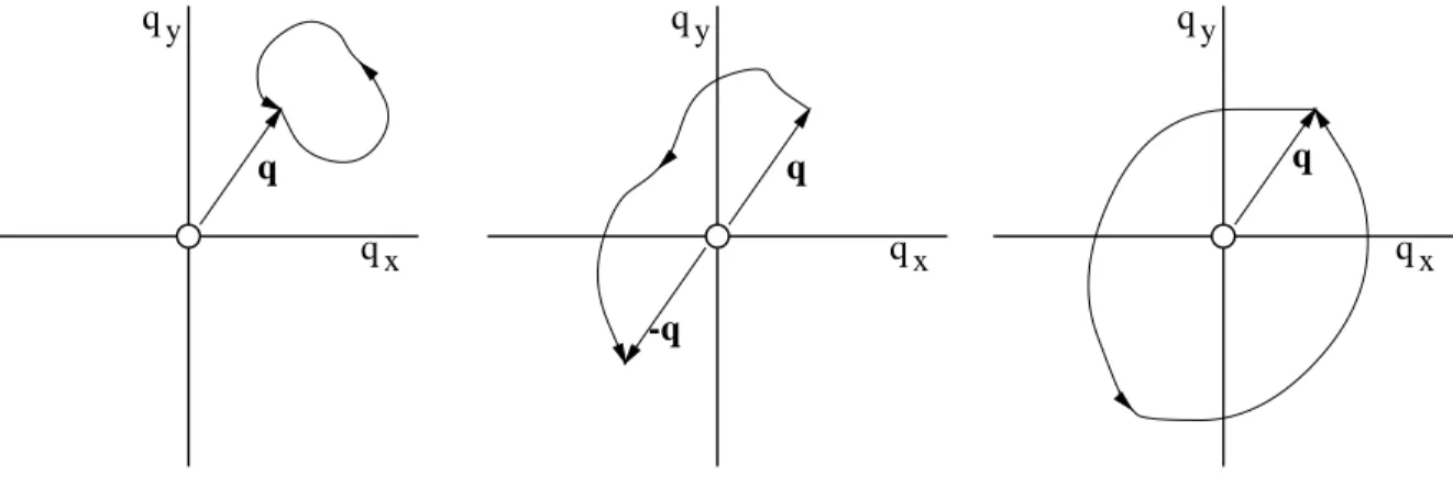
Once again, the PI separates into distinct topological classes, but there are now an infinity of possible classes. To see this, consider the three paths depicted in Figure 8, where for simplicity we restrict to the case where the initial and final configurations are the same.
It is important to remember that drawing paths in the plane is somewhat misleading: as in three dimensions, opposite points are identified, so that a path from any point to the diametrically opposite point is closed.
x qx qx
qy qy qy
q
q q
q
-q
Figure 8: Three topologically distinct paths in two dimensions.
The first and second paths are similar to the direct and exchange paths of the three- dimensional problem. The third path, however, represents a distinct class of path in two dimensions. The particles circle around each other, returning to their starting points.
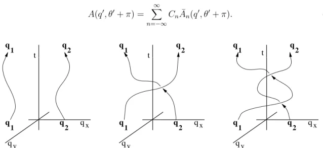
It is perhaps easier to visualize these paths in a three-dimensional space-time plot, where the vertical axis represents time and the horizontal axes represent space (Figure 9).
It is clear that in the third path the particle initially at q1 returns to q1, and similarly for the other particle: this path does not involve a permutation of the particles. It is also clear that this path cannot be continuously deformed into the first path, so it is in a distinct topological class. (It is critical here that we have excised the origin in relative coordinates – i.e., that we have disallowed configurations where the two particles are at the same point in space.)
4 TOPOLOGY AND PATH INTEGRALS 21 The existence of this third class of paths generalizes in an obvious way, and we are led to the following conclusion: the paths starting and finishing at relative position q can be divided into an infinite number of classes of paths in the plane (minus the origin); a class is specified by the number of interchanges of the particles (keeping track of the sense of each interchange). This is profoundly different from the three-dimensional case, where there were only two classes of paths: direct and exchange.
If we characterize a path by the polar angle of the relative coordinate, this angle is nπ in the nth class, where n is an integer. (For the three paths shown above, n = 0, 1, and 2, respectively.)
We can write
A(q, T;q,0) =
X∞
n=−∞
A¯n(q, T;q,0),
where ¯An is the covering-space PI considering only paths of change of polar angle nπ.
This path integral can again be generalized to A(q, T;q,0) =
X∞
n=−∞
CnA¯n(q, T;q,0),
Cn being phases. Since each ¯An satisfies the Schroedinger equation, so does this generaliza- tion.
Again, a restriction on the phases arises, as can be seen by the following argument. Let us relax the condition that the initial and final points are the same; let us denote the final point q′ by its polar coordinates (q′, θ′). Writing A(q′, θ′)≡A(q′, T;q,0), we have
A(q′, θ′) =
X∞
−∞
CnA¯n(q′, θ′).
Now, we can change continuously θ′ →θ′ +π, yielding A(q′, θ′+π) =
X∞
n=−∞
CnA¯n(q′, θ′+π). (26)
1 q
2 q1
q1 q
2 q1
q1 q
2 q1
q2 q
2 q
2
qx qx
qy qy
q
q x
t
qy
t t
Figure 9: Spacetime depiction of the 3 paths in Figure 8.
4 TOPOLOGY AND PATH INTEGRALS 22 Two critical observations can now be made. First, the final configuration is unchanged, so A(q′, θ′+π) can differ fromA(q′, θ′) by at most a phase:
A(q′, θ′+π) =e−iφA(q′, θ′).
Second, ¯An(q′, θ′+π) = ¯An+1(q′, θ′), since this is just two different ways of expressing exactly the same quantity. Applying these two observations to (26),
e−iφ
X∞
n=−∞
CnA¯n(q′, θ′) =
X∞
−∞
CnA¯n+1(q′, θ′)
=
X∞
−∞
Cn−1A¯n(q′, θ′). (27) Equating coefficients of ¯An(q′, θ′), we get
Cn=eiφCn−1. Choosing C0 = 1, we obtain for the amplitude
A=
X∞
−∞
einφA¯n, (28)
which is the two-dimensional analog of the three-dimensional result (21).
The most important observation to be made is that there is no longer a restriction on the angle φ, as was the case in three dimensions. We see that, relative to the “naive” PI (that with φ= 0), the class corresponding to a net number n of counter-clockwise rotations of one particle around the other contributes with an extra phase expinφ. If φ = 0 or π, this collapses to the usual cases of Bose and Fermi statistics, respectively. However in the general case the phase relation between different paths is more complicated (not determined by whether the path is “direct” or “exchange”); this new possibility is known as fractional statistics, and particles obeying these statistics are known as anyons.
Anyons figure prominently in the accepted theory of the fractional quantum Hall effect, and were proposed as being relevant to high-temperature superconductivity, although that possibility seems not to be borne out by experimental results. Perhaps Nature has other applications of fractional statistics which await discovery.
4.3 Magnetic Monopoles and Charge Quantization
All experimental evidence so far tells us that all particles have electric charges which are integer multiples of a fundamental unit of electric charge, e.6 There is absolutely nothing wrong with a theory of electrodynamics of particles of arbitrary charges: we could have particles of chargeeand√
17e, for example. It was a great mystery why charge was quantized in the early days of quantum mechanics.
In 1931, Dirac showed that the quantum mechanics of charged particles in the presence of magnetic monopoles is problematic, unless the product of the electric and magnetic charges
6The unit of electric charge is more properlye/3, that of the quarks; for simplicity, I will ignore this fact.
4 TOPOLOGY AND PATH INTEGRALS 23 is an integer multiple of a given fundamental value. Thus, the existence of monopoles implies quantization of electric charge, a fact which has fueled experimental searches for and theoretical speculations about magnetic monopoles ever since.
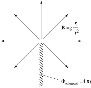
We will now recast Dirac’s argument into a modern form in terms of PIs. A monopole of charge g positioned at the origin has magnetic field
B =gˆer r2.
As is well known, this field cannot be described by a normal (smooth, single-valued) vector potential: writing B = ∇ × A implies that the magnetic flux emerging from any closed surface (and thus the magnetic charge contained in any such surface) must be zero. This fact makes life difficult for monopole physics, for several reasons. Although classically the Maxwell equations and the Lorentz force equation form a complete set of equations for particles (both electrically and magnetically charged, with the simple addition of magnetic source terms) and electromagnetic fields, their derivation from an action principle requires that the electromagnetic field be described in terms of the electromagnetic potential, Aµ. Quantum mechanically, things are even more severe: one cannot avoid Aµ, because the coupling of a particle to the electromagnetic field is written in terms ofAµ, not the electric and magnetic fields.
Dirac suggested that if a monopole exists, it could be described by an infinitely-thin and tightly-wound solenoid carrying a magnetic flux equal to that of the monopole. The solenoid is semi-infinite in length, running from the position of the monopole to infinity along an arbitrary path. The magnetic field produced by such a solenoid can be shown to be that of a monopole plus the usual field produced by a solenoid, in this case, an infinitely intense, infinitely narrow tube of flux running from the monopole to infinity along the position of the solenoid (Figure 10). Thus except inside the solenoid, the field produced is that of the monopole. The field inside the solenoid is known as the “Dirac string”. The flux brought
πg
solenoid=4 Φ
er r2 B =g
Figure 10: Monopole as represented by a semi-infinite, infinitely tightly-wound solenoid.