arXiv:1401.5107v1 [cs.LO] 20 Jan 2014
B¨ uchi Types for Infinite Traces and Liveness
Martin Hofmann1and Wei Chen2
1 LMU Munichmartin.hofmann@ifi.lmu.de
2 School of Informatics, University of Edinburgh
Abstract. We develop a new type and effect system based on B¨uchi automata to capture finite and infinite traces produced by programs in a small language which allows non-deterministic choices and infinite recursions. There are two key technical contributions: (a) an abstraction based on equivalence relations defined by the policy B¨uchi automata, the B¨uchi abstraction; (b) a novel type and effect system to correctly capture infinite traces. We show how the B¨uchi abstraction fits into the abstract interpretation framework and show soundness and completeness.
1 Introduction
A great range of techniques and tools have been developed and studied for the prediction of program behaviours without actually running the program [15,9,26,28,10,11]. One of them, originating from type inference in functional programming languages, is the type and effect discipline [25]. As a refinement of type systems in programming languages, types are annotated with information characterizing dynamic behaviours of programs—effects. As a result, a well- typed program satisfies some properties regarding its side-effects as well. This type-based technique has been used for all kinds of static analysis of programs, e.g. flow analysis [27], dependency analysis [1], resource allocation analysis [32], and amortised analysis [21,20], etc. In particular, a type and effect system was developed by Grabowski et al. [18] to verify that a particular programming guideline for secure web-programming has been adhered to. Generalizing from this, one could model a programming guideline as a property of traces that a program might have, where traces are sequences of events that are issued by a certain instrumentation of the program with special event-issuing operations.
This instrumentation would be part of the formalised guideline. A finite state machine would then be used to specify the set of acceptable traces. Most policies involve safety properties which can be assessed by examining finite portions of traces. In some cases, however, properties pertaining to liveness and fairness [4]
can become relevant. For instance, a guideline could be that calls to appropriate logging functions must be made again and again or that event (sic!) handlers should not become stuck, e.g. in the Java Swing framework.
This motivated us to investigate the possibility of using type systems in this situation as well. Our aim is not to offer new algorithms for deciding certain temporal properties or indeed to compete with the existing methods which are numerous [15,9,26,6], but to extend the reach of type systems. Our solution goes,
however, beyond a simple reformulation of an existing algorithm; the abstract domain based B¨uchi automata may well be useful in its on right and is an original contribution of this work.
For the sake of simplicity, we introduce and study a small language consisting of recursive first-order procedures and non-deterministic choices. The language explicitly allows infinite recursions. In this language, except for primitive pro- cedures which have events as arguments, other procedures have no inputs. We define trace semantics which formalize finite and infinite traces generated by programs in this language. We also remark that in essence our language is the same as the pushdown systems that have been studied in detail by a number of authors [34,6,30]. Similar trace semantics were also studied by the Cousots [12]
as a specific case of abstract interpretation.
Once a satisfactory type system for such a simple language has been found, it can be combined with known techniques [5,29] to scale to a type system for a large fragment of Java or similar languages. Alternatively, one can use our simple language as a target of a preliminary abstraction step.
Then, we develop the B¨uchi type and effect system to capture correctly finite and infinite traces. Since branching is non-deterministic in our language, we can even establish a completeness result. Completeness, of course, will be lost, once we re-introduce data-dependent branching.
As a demonstration, we extend the B¨uchi type and effect system for this small language to a B¨uchi type and effect system for Featherweight Java with field update [5].
The main technical contribution of this paper is the design of an abstract domain in the sense of abstract interpretation [10,11] based on B¨uchi automata or rather a mild extension of those allowing infinite as well as finite words. The proofs of soundness and completeness of the type system are based on clear-cut lattice-theoretic properties of this abstraction.
As in the finitary case, thisB¨uchi abstractionis based on equivalence relations on finite words generated by the policy B¨uchi automaton. Abstracted effects are no longer sets of such equivalence classes, but rather sets of pairs of the form (U, V) with U, V classes and representing the infinitary language U Vω. While such pairs appear in B¨uchi’s original complementation construction for B¨uchi automata [7] and have subsequently been used by a number of authors [31,14,19], they have never been used in the context of type systems and abstract interpretation.
1.1 Related work
As already mentioned, our language is equivalent to pushdown systems for which model-checking of temporal properties has been extensively studied [34,30,16,8].
Pushdown systems, on the other hand, are special cases of higher-order recursion systems introduced by Knapik et al. [23] and extensively studied by Ong and his collaborators, e.g. [3,24].
The latter work [24] also casts model checking into the form of a type system and is thus quite closely related to our result. More precisely, from an alternating parity automaton a type system for higher-order recursion schemes is derived
such that a scheme is typable iff its evaluation tree would be accepted by the automaton. In this way, in particular all mu-calculus definable properties of the evaluation tree become expressible. Regarding trace languages as opposed to tree properties alternating parity automata are equivalent to B¨uchi automata since both capture the (ω−)regular languages. Thus for the trace language of interest here the system from loc.cit. is equal in expressive power to our type system.
The difference is that Kobayashi and Ong’s system has a much more seman- tic flavour not unlike the intersection type systems used to characterise strong normalisation. More concretely, the well-formedness condition for recursions in that system requires the solution of a parity game whose size is proportional to the size of the program (number of function symbols to be precise) which is known to be equivalent to model checking trees against mu-calculus formulas.
Our type system, on the other hand, deviates from the standard type systems used in programming and program analysis only very slightly; instead of the usual recursion rule (which is clearly unsound in the context of liveness) we use a rule involving a type variable. No further semantic conditions need to be checked once of course the given B¨uchi automaton has been analysed and preprocessed.
We can also mention that our method and approach are rather different.
While loc.cit. uses games and automata we rely on the recently re-popularised [17,2] Ramseyian approach to the study ofω-regular language and automata.
Another recent work on the use of types for properties of infinite traces is [22] which embeds formulas of Linear Temporal Logic into types in the context of functional reactive programming. This work, however, relies on an encoding of linear temporal logic in first-order logic with integers, e.g., one models “the eventxoccurs infinitely often” as a formula like∀i∃j.xj wherexj refers to that the eventxissues at the timej. Dependent types are being used to turn this into a type system, but questions of inference and decidability are not considered.
The discussed works [24,22] are—to our knowledge—the only attempts at extending the range of typing beyond safety properties.
1.2 Outline
In the next section we define a simple first-order language with parameter- less recursive procedures and non-deterministic branching (meant, of course, to abstract ordinary conditionals). An alphabet of events Σ is assumed and for each event a ∈ Σ a primitive procedure o(a) is available that outputs a and has no effect on control flow or state. Programs are toplevel mutually recursive definitions of parameterless procedures comparable to the C-language. Given a program, any expression then admits a set of finite and infinite words overΣ—
the traces of terminating and nonterminating computations of the program. We distinguish finite traces stemming from terminating execution from finite traces stemming from nonterminating but “unproductive” executions. Thus, for every expressione(relative to a well-formed program) and tracew∈Σ≤ω=Σ∗∪Σω we define a judgemente⇓wmeaning thateadmits a terminating execution with tracew(necessarilyw∈Σ∗ then) and another judgemente⇑wmeaning that eadmits a nonterminating computation with tracew. In this case bothw∈Σ∗
andw∈Σωare possible. Formally, this is defined by introducingXevents that are repeatedly issued so that any nonterminating computation will have an in- finite trace with X events. The official trace semantics (e ↓ w and e ↑ w) is then defined by discarding theseXevents. We then discuss alternative ways for defining the trace semantics and emphasize that it is merely meant to formalize the intuitively clear notion of event trace occurring during a computation.
In Section 3 we then define a type-and-effect system whose effects are pairs (U, V) withU ⊆Σ∗ andV ⊆Σ≤ω. Semantically, an expression has effect (U, V) when e ↓ w implies w ∈ U and e ↑ w implies w ∈ V. The typing rules are given in Figure 2. We notice here that for theU-part (terminating computation) the typing rules are as usual; one “guesses” a type for a recursively defined procedure and justifies it for its body. The rule for the nonterminating “V-part”
is different. One assumes a type (and effect) variable for the recursive calls, typechecks the body and then takes the greatest fixpoint of the resulting type- and-effect equation.
With an ordinary recursive typing rule it would be possible to infer an ef- fect like (∅,(a∗b)ω) (“infinitely oftenb”) for the programm() =o(a);m() which is unsound. We then establish soundness (Theorem 1) and completeness (Theo- rem 2) for this type-and-effect system. In particular, this shows that the proposed handling of recursive definitions does indeed work.
The type system is at this level, however, of limited use since the effects are infinitary objects. Therefore, in Section 4 we introduce an abstraction of this type-and-effect system where effects are taken from a fixed finite set. This finite set is calculated from an a priori given B¨uchi automaton and effects still denote pairs of finite and possibly infinite languages, but no longer is any such pair denotable.
Our main result Theorem 5 then asserts that if the set of all traces of an expression is accepted by the given B¨uchi automaton then this is provable in the abstracted type-and-effect system. So, no precision is lost in this sense. Of course, we also have an accompanying soundness theorem (Theorem 4) for the abstract type-and-effect system.
These results can be modularly deduced from soundness and completeness for the infinitary type-and-effect system (Thms 1 and 2) with the help of lattice- theoretic properties of the abstraction that are established in Section 4.2. In particular, we have a Galois connection between the lattice of all languages and the lattice of language denotations in the abstract type system and all operations needed in the typing rules, in particular least and greatest fixpoints can be correctly rendered on the level of the abstractions.
The crucial building block is the ability to compute abstractions of greatest fixpoints needed for recursive definitions entirely on the level of the abstracted types. This requires the combination of a combinatorial lemma (Lemma 8) with known covering properties (Lemma 3) of the abstractions which follow from Ramsey’s theorem. Section 4.1 and Section 4.2 contain these lattice-theoretic results. We consider the discovery of this abstract lattice obtained from a B¨uchi automaton an important result of independent interest.
Section 4.2 then contains the actual definition of the abstracted type-and- effect system and its soundness and completeness theorems which, as already mentioned, then are direct consequences of earlier results. Section 4.3 discusses automatic type inference and its complexity.
An Appendix contains several worked out examples that did not fit into the main text and omitted proofs. We also sketch there, as a demonstration, a combination of an existing region-based type and effect system for Featherweight Java with field update [5] with B¨uchi types.
2 Trace Semantics
The syntax of expressions is given bye ::= o(a)|f |e1; e2|e1 ?e2 where o(a) is the only primitive procedure which generates an event a taken from a fixed alphabetΣof events andf ranges over procedures defined by expressions.
Parentheses are used to eliminate ambiguity. We assume that the operator ; is right-associative and has higher priority than the operator ?. As an example, we can define proceduresf andgas:f =o(b) ?o(a) ; gandg=f; g; (o(b) ?o(a)).
Formally, thus a program consists of a finite set of procedure identifiersF and for eachf ∈ Fan expressionef definingf where calls to procedures fromF are allowed and in particular,f may occur recursively inef.
From now on, we fix such a programP= (F,(ef)f∈F) and call an expression ewell-formed if it uses calls to procedures fromF only.
Since the operator ? is non-deterministic and non-primitive procedures have no arguments, stacks and heaps are not needed at this level of abstraction.
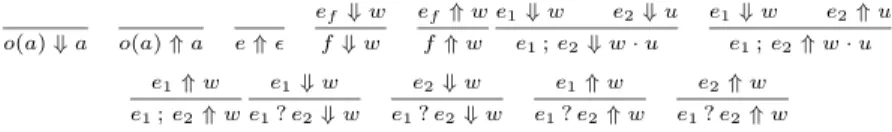
LetΣ≤ωbe the set of all finite and infinite sequences generated from the set Σof primitive events. We call an elementwinΣ≤ω atrace. Given traceswand u, we define the concatenationw·uas:wuifw∈Σ∗ and w ifw∈Σω where Σ∗ andΣω are respectively sets of all finite and infinite sequences over Σ. So, Σ≤ω =Σ∗∪Σω and Σ∗ = Σ+∪ {ǫ}. As usual, we may write wu instead of w·u. We are concerned with finite prefixes of the trace generated by a given expression. We call them observed traces. Notice that all observed traces are in Σ∗. Letef be the definition (a well-formed expression) off. The observed trace semantics is given in Figure 1. We write e ⇓ w to mean that the finite trace
o(a)⇓a o(a)⇑a e⇑ǫ
ef⇓w f⇓w
ef⇑w f⇑w
e1⇓w e2⇓u e1;e2⇓w·u
e1⇓w e2⇑u e1;e2⇑w·u e1⇑w
e1;e2⇑w e1⇓w e1?e2⇓w
e2⇓w e1?e2⇓w
e1⇑w e1?e2⇑w
e2⇑w e1?e2⇑w
Fig. 1.The Observed Trace Semantics
generated byeisw. In particular,eterminates. We writee⇑wto mean thatw is a finite prefix of the trace generated bye. Let the notationu4wdenote that uis a finite prefix ofw. We have: if e⇓wore⇑w, then for allu4w,e⇑u.
We now turn to define infinite traces of non-terminating programs. Unfor- tunately, the observed trace semantics does not contain enough information for this. Let us consider the following definitions:f =o(a), g = (o(a) ; h) ?o(a), and h= h. Notice that the observed traces of f and g are exactly the same.
However, the procedureg has a path leading to an unproductive infinite recur- sion h while f is non-recursive. In order to fix this problem, let us introduce the extended setΣ⊎ {X} of events and use (Σ⊎ {X})≤ω for the set of allex- tended traces. The observed extended trace semantics is same as the observed trace semantics except for the rule for function application in which a X-event is automatically generated. That is, f⇑efX⇑w·w. The specific symbolX is added to the beginning of trace w ofef. By doing this, unproductive infinite recursions can be distinguished from productive cases by observed extended tracesX∗.
For all observed extended tracesw, letθ(w) denote the trace obtained fromw by removing all Xs. Based on the observed extended trace semantics, we define trace semantics as follows.
Definition 1 (Trace Semantics).For all expressionseand extended tracesw in (Σ⊎ {X})≤ω,
e↓w ≡ ∃w′ ∈(Σ⊎ {X})∗. e⇓w′∧w=θ(w′);
e↑w ≡ ∃w′ ∈(Σ⊎ {X})ω.(∀u4w′. e⇑u) ∧ w=θ(w′).
We say wis a trace of eif e↓wore↑w.
Notice that ife↓w, thenwis inΣ∗ and all executions ofeterminate. Ife↑w, then wis inΣ≤ω and all executions ofedo not terminate. In our definition of trace semantics, the symbol X is introduced to distinguish finite traces gener- ated by terminating programs and non-terminating programs. When the trace semantics is well-defined, we remove allXs.
We remark that this way of defining the semantics is one of several possibil- ities; alternatives would consist of using a small step operational semantics or a coinductive definition. For instance, Cousot et al [12] define a generalization of structured operational semantics (G∞SOS), is used to describe the finite and infinite executions of programs. At the end of the day we need to define the two judgementse↓wmeaning thateterminates with tracewso, necessarilyw∈Σ∗ ande↑wmeaning thatedoes not terminate (runs forever) and its trace isw. In this case,wmay either be an infinite word (w∈Σω) or a finite word (w∈Σ∗) in which casee’s evaluation gets stuck in an infinite loop butedoes not output events during this loop.
An important fine point is that at our level of abstraction programs have a finite store which means that by K¨onig’s lemma “arbitrarily long” and “infinitely long” coincide. In a language allowing the nondeterministic selection of integers we could write a program that admits traces (outputtingas) of any finite length but not having an infinite trace. Then, our trace semantics would erroneously ascribe the trace aω to such a program. But, fortunately, in our situation this does not occur. As a result, for some language extensions, one may need to consider more complicated formal definitions of trace semantics. This would,
however, have no influence on the type system we define and only very little influence on correctness proofs.
3 Type and Effect System
In this section, we develop a type and effect system that captures the set of finite and infinite traces of a program. We also prove that this system is sound and complete. This system uses arbitrary languages for effect annotations and as such is not yet suitable for practical use let alone automatic inference. Later, in Section 4 we define a finitary abstraction of this system which still allows one to check soundly and completely whether the traces of a given program are accepted by a fixed B¨uchi automaton.
Definition 2 (Effect).Let U be a subset ofΣ∗ andV be a subset ofΣ≤ω. An effect of a given expression e is a pair(U, V)satisfying: (a) if e↓w, then wis in U; (b) if e ↑ w, then w is in V. We use the notation e & (U, V) to denote that (U, V)is an effect of e.
Let X be a set of variables. Let V(X) range over expressions of the form:
S
X∈X(AX ·X)∪B with AX ⊆ Σ∗ and B ⊆ Σ≤ω. We abbreviate X\ {X} by X−X and thus use the notation V(X−X) to denote expressions of the form: S
Y∈X−{X}(AY ·Y)∪B. We use the symbol X itself for the expression where B=∅,AX ={ǫ}, andAY =∅ for allY in X−X. We define the follow- ing operations on these expressions: A·V(X) = S
X∈X((A·AX)·X)∪(A·B) and V(X)∪V′(X) = S
X∈X((AX∪A′X)·X)∪(B∪B′) where A is a subset of Σ∗. Given an assignment function η : X → P(Σ≤ω) that assigns a set of traces to each variableX in X, we obtain for each expression V(X) a language V(η)⊆Σ≤ωby substitutingη(X) for each variableX.
We define Aω as the set of all words of the form w = w0w1w2· · ·wi· · · where wi ∈ A. Note that Aω ⊆ Σ≤ω. Let ∆ be an environment that is a set of expressions of the form: f & (U, X) withf a non-primitive procedure, U a subset ofΣ∗, andX a variable inXsuch that iff & (U, X) andg & (V, Y) both occur in ∆ then X 6= Y. With the above definitions, we define the type-and- effect systemin Figure 2. An environment∆is justified if for allf & (U, X) in
∆⊢o(a) & ({a},∅)
∆⊢e1& (U1, V1(X)) ∆⊢e2& (U2, V2(X))
∆⊢e1;e2& (U1·U2, V1(X)∪U1·V2(X))
∆⊢e1& (U1, V1(X)) ∆⊢e2& (U2, V2(X))
∆⊢e1?e2& (U1∪U2, V1(X)∪V2(X)) ∆, f & (U, X)⊢f& (U, X)
∆, f& (U, X)⊢ef & (U, A·X∪V(X−X))
∆⊢f& (U, A∗·V(X−X)∪Aω)
Fig. 2.The Type and Effect System
∆ one has∆⊢ef & (U, A·X∪V(X−X)) for someA, V(X−X). A justified environment can be extended as follows:
Lemma 1. Given a justified environment∆such that∆, f & (U, X)⊢ef& (U, A·
X∪V(X−X)), then the extended environment ∆, f & (U, X)is also justified An assignment function ηsatifies an environment∆if wheneverf & (U, X) in
∆ andf ↑wthenw∈η(X). Let us use the notationη|=∆to denote that the environment∆ is justified and that the assignment functionη satisfies∆.
Lemma 2. Given an environment ∆ and an assignment function η satisfying thatη|=∆, letη′ be an extensionη[X 7→V]ofη such thatf ↑wimpliesw∈V for all traces w. If we have the derivation: ∆, f & (U, X) ⊢ ef & (U, A·X ∪ V(X−X)), thenη′ |=∆, f & (U, X).
Theorem 1 (Soundness). Given an environment∆ and an assignment func- tion η satisfying that η |= ∆, for all derivations: ∆ ⊢ e & (U, V(X)) of an expressione, we have: e↓wimplies w∈U ande↑wimpliesw∈V(η).
Proof. The only interesting case is that for the last rule in Figure 2 which relies on Lemma 2. For more details, see Appendix B.
Corollary 1. For all derivations ⊢ e & (U, V) of an expression e, we have:
e↓wimpliesw∈U ande↑wimpliesw∈V.
Fix for each non-primitive proceduref ∈ F a unique variable Xf. If A = (Af)f is a family of languages with Af ⊆ Σ∗ define the corresponding en- vironment ∆(A) as to contain the bindings f & (Af, Xf). For each function bodyef we can now derive using the rules except the last one a unique typing
∆(A)⊢ ef & . . .. The passage fromA to C = (Cf)f defines a monotone op- erator Φ on the latticeP(Σ)F. IfB is the least fixpoint of this operator then
∆(B) is justified and we get the judgements ∆(B) ⊢ ef & (Bf, V(X)). Suc- cessive application of the last rule then gives judgements⊢f & (Uf, Vf) and a direct induction shows that in factUf ={w|f ↓w} andVf ={w|f ↑w}. We have thus shown:
Theorem 2 (Completeness). The judgements ⊢ f : ({w | f ↓ w},{w | f ↑ w})are derivable for each f.
We have kept the proof of this theorem in the running text since the monotone operatorΦis still needed later.
4 B¨ uchi Type and Effect System
Based on equivalence relations on finite words defined by the policy B¨uchi automata, we introduce an abstraction of languages of finite and infinite words:
the B¨uchi abstraction. We place this abstraction into the framework of abstract interpretation and show that crucial operations, namely concatenation, least fixpoint, and infinite iteration ((−)ω) can be computed on the level of the ab- straction. We also show that the abstraction does not lose any information as far as acceptance by the fixed policy automaton is concerned. This then allows us to replace the infinitary effects in the previous type system by their finite abstraction and thus to obtain a type-and-effect system which is decidable with
low complexity (in the program size) and yet complete. The soundness and com- pleteness of this system follow directly from lattice-theoretic properties of this B¨uchi abstraction (Lemma 3 and Theorem 3).
4.1 Extended B¨uchi Automata
Given an expressione, our goal is to verify that the set T(e) of all traces generated byesatisfies some property. We use a mild extension of the standard B¨uchi Automata which we callextended B¨uchi automata:
Definition 3. An extended B¨uchi Automaton is a quadrupleA= (Q, Σ, δ, q0, F) whereQis a finite set of states,Σis an alphabet; hereafter always required to be equal to the fixed alphabet of events;δ:Q×Σ→ P(Q)the transition function, the initial stateq0∈Q, and the setF ⊆Qof final states. The languageL(A)of A is defined as: the set of all finite words by which a final state can be reached from the initial state and all infinite words for which there is a path which starts from the initial state and goes through final states infinitely often. Thus,L(A)is the union ofA’s language when understood as a traditional NFA and its language when understood as a traditional B¨uchi automaton.
Following B¨uchi’s original works we use equivalence relations defined by ex- tended B¨uchi automata themselves to obtain finite representations ofU andV. We writeq w q′ to mean that the stateq′ is reachable from the stateqby using the finite wordw. Letq wF q′ denote that by using the finite wordw, the state q′ can be reached from the stateqin such a way that a final state is visited on the way. In particular,q w q′ with q∈F or q′ ∈F impliesq wF q′. Formally, we haveq wF q′ iff there existsq′′∈F andu, v such thatw=uvandq u q′′
andq′′ v q′.
For nonempty wordsw, u∈Σ+ we define
w∼u ≡ ∀p, q∈Q . p w q⇔p u q ∧ p wF q⇔p uF q .
We write [w] for the equivalence class ofw∈Σ+and additionally let [ǫ] stand for {ǫ}. We writeQ forΣ+/∼ ⊎ {[ǫ]}. ThusQ comprises the∼-equivalence classes and a special class for the empty word.
We notice that ifw∼uandw′∼u′ thenww′ ∼uu′. As a result concatena- tion is well-defined on equivalence classes, thusΣ+/∼becomes a semigroup and Qa monoid. The following Lemma is a straightforward consequence of standard results about B¨uchi automata [33].
Lemma 3. Fix an extended B¨uchi automaton A= (Q, Σ, δ, q0, F), (a) Qis finite and its elements are regular languages;
(b) for all classes C inQ,C∩L(A)6=∅ impliesC⊆L(A);
(c) for all classes C andD inQ,CDω∩L(A)6=∅implies CDω⊆L(A);
(d) for every wordw∈Σ≤ωthere exist classes C, D∈ Q so thatw∈CDω and CD=C andDD=D.
The sets CDω (with CD = C and DD =D) thus behave almost like classes themselves, but an important difference is that they may nontrivially overlap.
IfCDω∩U Vω6=∅ then in general one cannot concludeCDω=U Vω. We also remark that Ramsey’s theorem is used in the proof of (d).
4.2 B¨uchi Abstraction
Lemma 3 shows that given an extended B¨uchi automatonA, without affecting property checking, we can use sets of classes inQto represent languages overΣ∗ and sets of pairs of classes (C, D) such thatCD=CandDD=Dto represent languages overΣ≤ω. Let us writeC:={(C, D)|C, D∈ Q∧CD=C, DD=D}.
Let us define the pre-abstraction function f : P(Σ≤ω) → P(C) and the pre- concretization functiong:P(C)→ P(Σ≤ω) as:f(V) ={(C, D)∈ C |CDω∩V 6=
∅}andg(V) =S
(C,D)∈VCDωrespectively. A setV ⊆ Cisclosed, iff(g(V)) =V. Explicitly, V is closed if wheneverU Vω∩CDω 6= ∅ for some (C, D) ∈ V and (U, V)∈ C then already (U, V)∈ V.
Clearly, for every set V ⊆ C there is a least closed superset and it is given by applying the closurefunction: c:P(C)→ P(C) which is defined as: c(V) = S∞
n=1(f◦g)n(V). We writeM≤ω={c(f(V))|V ⊆Σ≤ω}for the set such closed subsets. The elements ofM≤ωwill serve as abstractions of languages overΣ≤ω. We also define explicitly M∗ = P(Q) to represent languages over Σ∗ but note that via the embedding C7→(C,{ǫ}) we could identifyM∗ with a subset ofM≤ω.
Lemma 4. BothM∗ andM≤ωare complete lattices with respect to inclusion.
From now on we call P(Σ∗) and P(Σ≤ω) theconcrete domains and M∗ and M≤ω the abstract domains. We introduce the following abstraction functions: α∗:P(Σ∗)→ M∗ andα≤ω:P(Σ≤ω)→ M≤ω, which are respectively defined as: α∗(U) ={C ∈ Q | C∩U 6=∅} and α≤ω(V) = c(f(V)). We also introduce the following concretization functions: γ∗ : M∗ → P(Σ∗) and γ≤ω : M≤ω → P(Σ≤ω), which are respectively defined as:γ∗(U) =S
C∈UCandγ≤ω(V) =g(V).
Lemma 5. The abstraction and concretization functions are monotone and form Galois connections, that is: α∗(U) ⊆ U iff U ⊆ γ∗(U), and α≤ω(V) ⊆ V iff V ⊆γ≤ω(V). Moreover, α∗(γ∗(U)) = U and α≤ω(γ≤ω(V)) = V so we have in fact a Galois injection. Furthermore, both abstraction and concretization func- tions preserve unions, least and greatest elements. The concretization functions also preserve intersections.
The next lemma shows that the abstraction is sufficiently fine for our purposes.
It is a direct consequence of the Galois connection and the fact thatL(A) itself is closed which in turn is direct from Lemma 3 (b) and (c).
Lemma 6. Let p∈ {∗,≤ω}. If L⊆Σp thenγp(αp(L))⊆L(A)iffL⊆L(A).
We now turn to define some new operators for the abstract domains. We have a concatenation operation onM∗ given pointwise, i.e. forU,U′ ∈ M∗, we define U ·U′={U U′|U ∈ U, U′∈ U′}. We also define a concatenation·:M∗×M≤ω→ M≤ωas follows:U ·V={(AC, D)|A∈ U ∧(C, D)∈ V}. Note thatACD=AC.
Lemma 7. If U ∈ M∗ andV ∈ M≤ω thenU · V ∈ M≤ω.
Theorem 3. The preservation properties listed in Table 1 are valid.
Most of these properties are direct and folklore or have been asserted earlier.
In the clause about least fixpoints denoted by lfp the operators Φ and F are supposed to be monotone operators onP(Σ∗)nandMn∗ for somen. The clause is then validated by straightforward application of lattice-theoretic principles.
Only preservation of (−)ω is a nontrivial and original result; it requires the following lemma.
α∗:P(Σ∗)→ M∗ α≤ω:P(Σ≤ω)→ M≤ω
α∗(⊤) =⊤ α≤ω(⊤) =⊤
α∗(⊥) =⊥ α≤ω(⊥) =⊥
α∗(U∪U′) =α∗(U)∪α∗(U′) α≤ω(V∪V′) =α≤ω(V)∪α≤ω(V′) α∗(U·U′) =α∗(U)·α∗(U′) α≤ω(U·V) =α∗(U)·α≤ω(V) α∗◦Φ=F◦α∗=⇒α∗(lfp(Φ)) =lfp(F) α≤ω(Uω) =α∗(U)ω
Table 1.Properties of the B¨uchi Abstraction
Lemma 8. Let (Li)i∈I be a family of classes (fromQ) and putP=Q
i∈ILi⊆ Σ≤ω, i.e., P comprises finite or infinite words of the form w1w2w3. . . where wi ∈Li for i ≥1. There exist classesU, V ∈ Q where U V =U, V V =V such that P ⊆U Vω.
Proof. Let w ∈ P and write w = w1w2w3· · ·wi· · · where wi ∈ Li. If w is a finite word then there exists n such that wi =ǫ (andLi = [ǫ]) for i ≥n and we can chooseU =L1. . . Ln−1 and V = [ǫ]. Otherwise, use Ramsey’s theorem as in the proof of Lemma 3 to obtain a sequence of indices i1 < i2 < i3 <
i4 < . . . and classes U, V where V 6= [ǫ] and V V = V, U V = U such that w1w2. . . wi1 ∈U, wi1+1. . . wi2 ∈V andwi2+1. . . wi3 ∈V and so on. It follows that U =L1L2. . . Li1 andV =Lik+1. . . Lik+1 for k≥1 and thusP ⊆U Vω as required.
Proof (of Theorem 3). It only remains to prove preservation of (−)ω. So, fix L ⊆ Σ∗. We want to show that α≤ω(Lω) = α∗(L)ω. Note that α∗(L)ω = α≤ω(γ∗(α∗(L))ω). The direction “⊆” is obvious from monotonicity; towards proving “⊇” assume (U, V) ∈ α≤ω(γ∗(α∗(L))ω). Since α≤ω(Lω) is closed, we may without loss of generality assume that U Vω∩γ∗(α∗(L))ω 6=∅. Pickw ∈ U Vω∩γ∗(α∗(L))ω and decomposew=w1w2. . . wherewi∈γ∗(α∗(L)). Define Li:= [wi] and apply Lemma 8 to obtainU′, V′ withQ
iLi⊆U′V′ω. Note that, sincew∈P, we haveU Vω∩U′V′ω6=∅.
Now, sincewi∈γ∗(α∗(L)), by the definition ofα∗, we must have thatLi∩L6=
∅. Choosew′i∈Li∩L. The wordw1′w′2. . . is then contained inLω∩U′V′ω, so (U′, V′)∈α≤ω(Lω) and, finally, (U, V)∈α≤ω(Lω) sinceα≤ω(Lω) is closed and U Vω∩U′V′ω6=∅.
Definition 4 (B¨uchi Effect).LetU be an element inM∗ andV be an element inM≤ω. The pair(U,V)is a B¨uchi effect of a given expression eif it satisfies:
(a) if e↓w, thenw∈γ∗(U); (b) if e↑w, thenw∈γ≤ω(V).
LetV(X) range over expressions of the form:S
X∈X(AX·X)∪ BwithAX ∈ M∗ and B ∈ M≤ω. We define the notation V(X−X) and operations on these expressions in the same way as we have done for expressions in the type and effect system in section 3. The definitions of justifiedness and satisfaction of environments and assignments are adapted to the B¨uchi type system mutatis mutandis. That is,∆is justified if for allf & (U, X) in∆one has∆⊢ef& (U,A·
X ∪ V(X−X)). It is satisfied by η if f & (U, X) in ∆ and f ↑ w implies w∈γ≤ω(η(X)).
With the above definitions, we introduce the B¨uchi type and effect system in Figure 3.
∆⊢Ao(a) & (α∗({a}),∅)
∆⊢Ae1& (U1,V1(X)) ∆⊢Ae2& (U2,V2(X))
∆⊢Ae1;e2& (U1· U2,V1(X)∪ U1· V2(X))
∆⊢Ae1& (U1,V1(X)) ∆⊢Ae2& (U2,V2(X))
∆⊢Ae1?e2& (U1∪ U2,V1(X)∪ V2(X)) ∆, f & (U, X)⊢Af& (U, X)
∆, f & (U, X)⊢Aef & (U,A ·X∪ V(X−X))
∆⊢Af& (U,A∗· V(X−X)∪ Aω)
Fig. 3.The B¨uchi Type and Effect System
By using properties of the B¨uchi abstraction in Table 1, from Theorems 1 and 2, we have that this system is sound and complete.
Theorem 4 (Soundness). Given an environment∆ and an assignment func- tion η satisfying thatη|=A∆, for all derivations: ∆⊢Ae& (U,V(X))of an ex- pressione, we have:e↓wimpliesw∈γ∗(U)ande↑wimpliesw∈γ≤ω(V(X)η).
Proof. It follows from the Galois connections in Lemma 5. In particular, U ⊆ γ∗(α∗(U)) andV ⊆γ≤ω(α≤ω(V)).
Theorem 5 (Completeness).Given a non-primitive proceduref, let T(f)be the set of all traces generated by f. There is a derivation ⊢Af & (Uf,Vf)such that T(f)⊆L(A)if and only ifγ∗(Uf)∪γ≤ω(Vf)⊆L(A).
Proof. Recall the monotone operator Φ from the proof of Theorem 2. Since Φ is built up from concatenation and union there is an abstract operatorF such that α∗ ◦ Φ=F ◦ α∗. Thusα∗(lfp(Φ)) =lfp(F) and therefore, the judgements
∆(α(B)) ⊢A ef & (α∗(Bf), α∗(V(X))) (again in keeping with the notation of that proof) are derivable in the B¨uchi type system. Using the preservation of (−)ω repeatedly, we then obtain the judgements ⊢A f & (α∗(Uf), α≤ω(Vf)) where Uf = {w | f ↓ w} and Vf = {w | f ↑ w}. Letting Uf = α∗(Uf) and Vf =α≤ω(Vf) the claim then follows using Lemma 6.
4.3 Type inference and complexity
Given that the abstract lattices and thus the set of types is finite, type inference is a standard application of well-known techniques. We therefore just sketch it here to give an idea of the complexity.
From a given program we can construct in linear time a skeleton typing derivation for the finitary effect annotations. The skeleton typing derivation contains variables in place of actual effect annotations; the number of these variables is linear in the program size. The side conditions of the typing rules then become constraints on these variables and any solution will yield a valid typing derivation. In quadratic time (assuming that M≤ω has constant size) we can then compute the least solution of these constraints using the usual iteration algorithms known from abstract interpretation. Once we have in this way obtained the finitary effect annotations we can then (in linear time) derive the infinitary ones using the (−)ω and infinitary concatenation operators on M≤ω.
Once the type of an expression has been found one can then check (in constant time) whether the language denoted by it is accepted by the policy automaton.
If we are interested in complexity as a function of the size of the policy automaton the situation is of course different. The important parameter here is the size of the abstract lattices since the number of iterations as well as the runtime of the algorithms for computing the abstractions of concatenation, union, infinite iteration are linear in this parameter. Ifnis the number of states of the policy automaton then the number of classes can be bounded by 22n2 since each class is characterised by two sets of pairs of states. The resulting exponential in n runtime of our algorithms is no surprise since the PSPACE- complete problem of universality of B¨uchi automata is easily reduced to type checking. We believe that by clever space management our algorithms can be implemented in polynomial space but we have not verified this.
On a positive note we remark that for a small policy automaton the set of classes is manageable as we see in the examples below. We also note that once the classes have been computed and the abstract functions tabulated one can then analyse many programs of arbitrary size.
5 Conclusions
We have developed a type-and-effect system for capturing possibly infinite traces of recursively defined first-order procedures. The type-and-effect system is sound and complete with respect to inclusion of traces in a given B¨uchi (“policy”) automaton. The effect annotations are from a finite set that can be effectively computed from the B¨uchi automaton. Type inference using constraint solving is thus possible. We emphasize that the resulting ability to decide satisfaction of temporal properties of traces is not claimed as a new result here; since it has long been known in the context of model checking. The novelty lies in the presentation as a type and effect system that follows the standard pattern of such systems. As we explain below, this opens the way for smooth integration with existing type-theoretic technology.
The proofs of soundness and completeness are organised in a modular fashion and decomposed into a type-theoretic part expressed in the form of an infinitary system (Section 3) and a lattice-theoretic part (Section 4.2). Concretely, this Section defines an abstract domain from any given B¨uchi automaton and derives crucial properties of this abstraction. We consider a contribution of independent interest. The finite part of this abstraction, i.e., M∗, is akin to the abstract domain proposed by Cousot et al [13] which also has finite abstraction values and its abstraction function preserves the least fixed point as well. The infinite part M≤ω is a new abstract domain with its abstraction function preserving not only least fixed points but also the new operator (−)ω. We remark here that the abstraction function does not preserve greatest fixed points so that the introduction of the (−)ω operator on the abstract domain is a necessary device. This extension makes the B¨uchi type and effect system powerful enough to capture and reason about infinitary properties like liveness and fairness.
We have sketched a combination of our simple type system with a generic type and effect system for class-based object-oriented languages. Other possible extensions are in the direction of effectful functional programming. The stan- dard notation for type-and-effect systems as described e.g. in Henglein and Niss’
survey [29] could be used for our effect system mutatis mutandis leading in par- ticular to function types like w →ǫ w′ where w, w′ are types and ǫ is a B¨uchi effect (element of our abstract lattice) describing the latent effect of a function.
Assuming that we only allow first-order recursive definitions the design of such a type system would be completely standard. For higher-order recursion some extra technical work would be needed to lift the last rule from Fig. 2 and its corresponding abstraction to this case.
It is this option of integration with expressive type systems that makes our abstraction so attractive and superior (in this context!) to classical methods based on model checking.
References
1. Mart´ın Abadi, Anindya Banerjee, Nevin Heintze, and Jon G. Riecke. A core cal- culus of dependency. POPL, pages 147–160. ACM, 1999.
2. Parosh Aziz Abdulla, et al. Advanced ramsey-based b¨uchi automata inclusion testing. CONCUR, LNCS 6901, pp 187–202. Springer, 2011.
3. Klaus Aehlig, Jolie G. de Miranda, and C.-H. Luke Ong. The monadic second order theory of trees given by arbitrary level-two recursion schemes is decidable.
TLCA, LNCS 3461 pp 39–54. Springer, 2005.
4. Bowen Alpen and Fred B. Schneider. Recognizing safety and liveness. Distributed Computing, 2(3):117–126, 1987.
5. Lennart Beringer, Robert Grabowski, and Martin Hofmann. Verifying pointer and string analyses with region type systems. COMLAN, 2013.
6. Ahmed Bouajjani, et al. Reachability analysis of pushdown automata: Application to model-checking. CONCUR, LNCS 1243, pp 135–150. Springer, 1997.
7. J. R. B¨uchi. On a decision method in restricted second order arithmetic. InLogic, Method, and Philosophy of Science, Stanford University Press, 1962.
8. Olaf Burkart and Bernhard Steffen. Model checking the full modal mu-calculus for infinite sequential processes. TCS, 221(1-2):251–270, 1999.
9. Edmund M. Clarke, et al. Counterexample-guided abstraction refinement. CAV, LNCS 1855, pages 154–169. Springer, 2000.
10. Patrick Cousot and Radhia Cousot. Abstract interpretation. POPL, pages 238–
252. ACM, 1977.
11. Patrick Cousot and Radhia Cousot. Abstract interpretation frameworks. J. Log.
Comput., 2(4):511–547, 1992.
12. Patrick Cousot and Radhia Cousot. Inductive definitions, semantics and abstract interpretation. In Ravi Sethi, editor,POPL, pages 83–94. ACM Press, 1992.
13. Patrick Cousot and Radhia Cousot. Formal language, grammar and set-constraint- based program analysis by abstract interpretation. InFPCA, pages 170–181, 1995.
14. Christian Dax, Martin Hofmann, and Martin Lange. A proof system for the linear timeµ-calculus. FSTTCS, LNCS 4337, pages 273–284. Springer, 2006.
15. E. Allen Emerson and Edmund M. Clarke. Characterizing correctness properties of parallel programs using fixpoints. ICALP, LNCS 85, pp 169–181. Springer, 1980.
16. Javier Esparza, et al Efficient algorithms for model checking pushdown systems.
CAV, LNCS 1855, pp 232–247. Springer, 2000.
17. Seth Fogarty and Moshe Y. Vardi. B¨uchi complementation and size-change termi- nation. Logical Methods in Computer Science, 8(1), 2012.
18. Robert Grabowski et al. Type-based enforcement of secure programming guidelines - code injection prevention at sap. FAST, LNCS 7140, pp 182–197. Springer, 2011.
19. M. Heizmann, N. Jones, and A. Podelski. Size-change termination and transition invariants. SAS, LNCS 6337, pp 22–50. Springer, 2010.
20. Martin Hofmann and Steffen Jost. Type-based amortised heap-space analysis.
ESOP, LNCS 3924, pp 22–37. Springer, 2006.
21. Martin Hofmann and Dulma Rodriguez. Automatic type inference for amortised heap-space analysis. ESOP, LNCS 7792, pp 593–613. Springer, 2013.
22. Alan Jeffrey. Ltl types frp: linear-time temporal logic propositions as types, proofs as functional reactive programs. PLPV, pages 49–60. ACM, 2012.
23. Teodor Knapik, Damian Niwinski, and Pawel Urzyczyn. Higher-order pushdown trees are easy. FoSSaCS, LNCS 2303 pp 205–222. Springer, 2002.
24. Naoki Kobayashi and C.-H. Luke Ong. A type system equivalent to the modal mu-calculus model checking of HORS. InLICS, pages 179–188. IEEE, 2009.
25. John M. Lucassen and David K. Gifford. Polymorphic effect systems. In Jeanne Ferrante and P. Mager, editors,POPL, pages 47–57. ACM Press, 1988.
26. Kenneth L. McMillan. Symbolic model checking. Kluwer, 1993.
27. Christian Mossin. Higher-order value flow graphs.PLILP, LNCS 1292, pp 159–173.
Springer, 1997.
28. Flemming Nielson, Hanne Riis Nielson, and Chris Hankin. Principles of program analysis (2. corr. print). Springer, 2005.
29. Benjamin C. Pierce. Advanced Topics in Types and Programming Languages. The MIT Press, 2004.
30. Stefan Schwoon. Model-Checking Pushdown Systems. PhD thesis, Technische Uni- versit¨at M¨unchen, 2002.
31. A. Prasad Sistla, et al. The complementation problem for b¨uchi automata with appplications to temporal logic. Theor. Comput. Sci., 49:217–237, 1987.
32. Peter Thiemann. Formalizing resource allocation in a compiler. Types in Compi- lation, LNCS 1473, pp. 178–193. Springer, 1998.
33. W. Thomas. Languages, automata and logic. In A. Salomaa and G. Rozenberg, editors,Handbook of Formal Languages, vol 3. Springer, 1997.
34. Igor Walukiewicz. Pushdown processes: Games and model checking. CAV, LNCS 1102, pp 62–74. Springer, 1996.
A Examples
Example 1. Consider the following definition:
f = o(b) ; o(a) ; f Suppose that we want to verify the property:
Every finite trace generated byf ends withb. Every infinite trace gener- ated byf contains infinite many bs.
We can use the following extended B¨uchi automatonAto formalize this property.
A: //?>=<89:;0
a
b **?>=<89:;/.-,()*+1
b
jj a
We have:
L(A) = (a∗b+)+∪(a∗b)ω.
By the definition of∼, we have thatQconsists of four equivalence classes: the set of empty word ([ǫ] ={ǫ}), the set of non-empty words consists ofa([a] =a+), the set of words ending withaand containing at least oneb([ba] = (a+b)∗a−a+= (a+b)∗b(a+b)∗a), the set of words ending withb([b] = (a+b)∗b). Further, the set C={(C, D)|C, D∈ Q ∧CD=C, DD=D}is as follows:
{([ǫ],[ǫ]),([a],[ǫ]),([a],[a]),([b],[ǫ]), ([b],[b]),([ba],[ǫ]),([ba],[a]),([ba],[ba])}
and abstractions ofL(A) are:
UL={[b]} ∈ M∗
VL={([b],[ǫ]),([b],[b]),([ba],[ba])} ∈ M≤ω .
By using the B¨uchi type and effect system defined in Figure 3, we have that (U,V) = (∅,({[ba]})ω) is a B¨uchi effect of f. Further,
V=α≤ω((γ∗({[ba]}))ω) ={([b],[b]),([ba],[ba])}.
So, T(ef) ⊆γ≤ω(V)⊆γ≤ω(VL). That is, all traces generated by f satisfy the target property. This coincides with our observation thatf does not generate any finite traces and the only infinite trace generated byf is (ba)ω which contains infinite manybs.
Example 2. Consider the following C-like program:
0 #define TIMEOUT 65536 1 while (true) {
2 i = 0;
3 while (i++ < TIMEOUT && s != 0) { 4 unsigned int s = auth(); /* o(a); */
5 } /* o(c); */
6 work(); /* o(b); */
7 }
We would like to verify that line 6 is executed infinitely often under the fairness assumption that the while loop 3 always terminates. To this end, we can annotate the above program by uncommenting the event-issuing commands and abstract the so annotated program as the definition:
f = g;o(b) ; f g = (o(a) ; g) ?o(c)
We are then interested in the property “infinitely manyb” assuming that “in- finitely oftenc” (fairness) or equivalently: “infinitely manybor finitely manyc.”
This property can be readily expressed as the following B¨uchi automaton
A: ?>=<89:;/.-,()*+2
a,b
?>=<89:;0a,b,coo
a,b,c
II
b **?>=<89:;/.-,()*+1
a,b,c
jj
By the definition of∼, we have that the setQconsists of the following equivalence classes:
[ǫ] ={ǫ} [a] ={a} [b] ={b} [c] ={c}
[aa] =a+a [ba] = (a+b)+a−[aa]
[ab] =a+b [bb] = (a+b)+b−[ab]
[cb] = (a+c)∗c(a+c)∗b
[bcb] = (a+b+c)∗c(a+b+c)∗b−[cb]
[cca] = (a+c)+c ∪ (a+c)∗c(a+c)∗a [bca] = (a+b+c)+c ∪
(a+b+c)∗c(a+b+c)∗a−[cca].
Further, the set Cconsists of the following pairs:
([ǫ],[ǫ]) ([a],[ǫ]) o ([b],[ǫ]) ([c],[ǫ]) ([aa],[ǫ]) ([ba],[ǫ]) ([ab],[ǫ]) ([bb],[ǫ]) ([cb],[ǫ]) ([bcb],[ǫ]) ([cca],[ǫ]) ([bca],[ǫ]) ([aa],[aa]) ([ba],[aa]) ([ba],[ba]) ([bb],[bb]) ([bcb],[bb]) ([bcb],[bcb]) ([cca],[aa]) ([cca],[cca]) ([bca],[aa]) ([bca],[ba]) ([bca],[cca]) ([bca],[bca]) Then, the abstractions ofL(A) are as follows:
UL=Q − {[ǫ]} ∈ M∗
VL=C − {([ǫ],[ǫ]),([cca],[cca]),([bca],[cca])} ∈ M≤ω .
By using the B¨uchi type and effect system, we get the effect ofg as the pair:
(Ug,Vg) = ({[c],[cca]},{([aa],[aa])}). Then, the effect of f is the pair (Uf,Vf) given as follows:
(∅,{([aa],[aa]),([bca],[aa]),([bcb],[bcb]),([bca],[bca])}).
SinceUf⊆ ULandVf ⊆ VL, we have that the program satisfies the property.
B Proofs
Proof. (of Theorem 1) We proceed by induction on the structure of the type and effect system. The only interesting case is that for the last rule in Figure 2. Let us show that if
f ↑w and ∆⊢f & (U, A∗·V(X−X)∪Aω), thenwis inA∗·V(η)∪Aω. We introduce the assignment functions:
ηn=
η[X 7→Σ≤ω] if n= 0 ;
η[X 7→A·Xηn−1∪ V(η)] if n≥1.
From Lemma 2, η0 |= ∆, f & (U, X). Assume that ηn |= ∆, f & (U, X). By inductive hypothesis, we have that for allef ↑w,wis in
A·Xηn ∪ V(X−X)ηn=A·Xηn ∪ V(X−X)η=Xηn+1 .
Further, by Lemma 2, ηn+1 |=∆, f & (U, X). By mathematical induction, we have thatηn |=∆, f & (U, X) for all natural numbersn. Defineηωas
η[X7→
∞
\
n=0
Xηn].
We getηω|=∆, f & (U, X). Notice thatηω(X) is equal toA∗·V(η) ∪ Aω. By the definition of|=,wis inA∗·V(η)∪Aω.
Proof. (of Lemma 3) a) and b) are obvious from the definition. Property c) coincides with b) when D={ǫ}. Otherwise, letw, w′ ∈CDω. Decompose w= w1w2w3. . . andw′ =w′1w2′w′3. . . so thatw1, w′1∈C andwi, w′i ∈D fori >1.
We have wi ∼w′i for alli so any accepting run for w yields an accepting run forw′ by the definition of∼. Property d) is again trivial whenw∈Σ∗ (choose C = [w] andD ={ǫ}) and otherwise appears already in B¨uchi’s work. For the record, write w=a1a2a3. . . withai ∈Σ and “colour” the set{i, j}withi < j with the∼-class ofaiai+1. . . aj−1. By Ramsey’s theorem there exists an infinite set of indices i1< i2< i3. . . and a class D so that [aik. . . aik+1−1] =D for all k >0. The claim follows with C:= [a1. . . ai2−1].
Proof. (Proof of Lemma 4) This is trivial forM∗which is a powerset lattice. As forM≤ω, one must show that unions and intersections of closed sets are again closed. So, let (Vi)i∈I be a family of closed sets. To argue that the union of this family is closed, suppose thatU Vω∩CDω6=∅for some (C, D) contained in that union. Then, (C, D)∈ Vi for somei, so (U, V)∈ Vi. SinceViis closed, (U, V) is contained in the union. As for the intersection, suppose thatU Vω∩CDω 6=∅ for some (C, D) contained in the intersection. Then, (C, D) ∈ Vi for all i, so (U, V)∈ Vifor alli. Since eachViis closed, (U, V) is contained in the intersection, too.
Proof. (Proof of Lemma 7) We need to show thatU · V is closed so suppose that U Vω∩ACDω 6=∅ whereA∈ U and (C, D)∈ V. We may assume that V 6= [ǫ]
for otherwise the claim is trivial. Decomposing the witnessing word, we get finite wordsx, ywherexy∈U andx∈A. Note thatU V =U. Thus,U =AY withY the class of y. As a result,Y Vω∩CDω6=∅, so (Y V, V)∈ V by closedness and finally, (U, V)∈ U · V sinceU =AY V.
C Region-Based B¨ uchi Type and Effect System
In order to make the B¨uchi type and effect system given in Section 4.2 more functional and effective in programming practices, by integrating with region types [25,29,5], we extend it to a region-based B¨uchi type and effect system for Featherweight Java with field update. Based on this, the future goal is to develop and implement a powerful type system for Java-like languages in which (ω)-regular properties of traces can be properly characterized for verification purposes.
C.1 Syntax
The syntax of an expression e in Featherweight Java with field update is given as follows:
x∈V ar f ∈F ld m∈M td C, D∈Cls
e::=o(a)|null|x| newC|x.f |x.f :=y |
x.m(y)|letx=e1in e2|if x=ythene1 elsee2
For the sake of simplicity, we omit primitive types and casting and assume that every expression is in let normal form. In the definition of the if-then- else expression, the expressionx = y denotes an unusual judgement between objects which is independent on booleans. The notationy denotes a sequence of variables.
Additionally, the expressiono is used to produce appealing events. It is a global primitive procedure which is not part of Featherweight Java with filed update. It is added as annotations to programs for the purposes of property characterization.
Let ∈ P(Cls×Cls) be the subclass relation between classes. Letf ields∈ Cls→ P(F ld) andmethods∈Cls→ P(M td) be mappings from a class to its fields and methods respectively. We use mtable ∈ Cls×M td ⇀ V ar×Expr to denote the method table which assigns to each method its definition, i.e., its formal parameters (a sequence of variables) and its body (an expression). With these definitions, a programP is given as follows:
P= (, f ields, methods, mtable)
Usual well-formedness conditions on methods are assumed to ensure the inheri- tance relation between same methods from different classes.
C.2 Operational Semantics
The operational semantics of an expressioneare given in form of:
(s, h)⊢e⇓v, h′ &w (s, h)⊢e⇑ &w
We usee⇓vto denote that the evaluation ofeterminates and the value isv. The notatione⇑ means that the evaluation ofedoesn’t terminate. A valuev∈V al of an expression is a locationl∈Locornull. A state (s, h) is consisted of a stack s ∈ V ar ⇀ V al which is a partial function assigning to each variable a value and a heap h∈Loc ⇀ Cls×(F ld ⇀ V al) which is a partial function assigning to each location a pair of a class and values assigned to fields of this class. In addition, as side effects, an infinite or a finite tracew which is generated from the set Σ of events by ordinary concatenations is attached to each evaluation.
The whole operational semantics is given as follows:
Prim-a
(s, h)⊢o(a)⇓null, h&a
Null (s, h)⊢null⇓null, h&ǫ Var(s, h)⊢x⇓s(x), h&ǫ
New l6∈dom(h) F = [f 7→null]f∈f ields(C)
(s, h)⊢newC⇓l, h[l7→(C, F)] &ǫ Get s(x) =l h(l) = (C, F)
(s, h)⊢x.f ⇓F(f), h &ǫ
Set
s(x) =l h(l) = (C, F) h′ =h[l7→(C, F[f 7→s(y)])]
(s, h)⊢x.f :=y⇓s(y), h′ &ǫ