First-order definable languages

Volker Diekert

Paul Gastin

1 Institut f¨ur Formale Methoden der Informatik Universit¨at Stuttgart

Universit¨atsstraße 38 70569 Stuttgart, Germany diekert@fmi.uni-stuttgart.de

2 Laboratoire Sp´ecification et V´erification Ecole Normale Sup´´ erieure de Cachan 61, avenue du Pr´esident Wilson 94235 Cachan Cedex, France Paul.Gastin@lsv.ens-cachan.fr

Abstract

We give an essentially self-contained presentation of some princi- pal results for first-order definable languages over finite and infinite words. We introduce the notion of a counter-free B¨uchi automaton;

and we relate counter-freeness to aperiodicity and to the notion of very weak alternation. We also show that aperiodicity of a regular

∞-language can be decided in polynomial space, if the language is specified by some B¨uchi automaton.

1 Introduction

The study of regular languages is one of the most important areas in formal language theory. It relates logic, combinatorics, and algebra to automata theory; and it is widely applied in all branches of computer sciences. More- over it is the core for generalizations, e.g., to tree automata [26] or to par- tially ordered structures such as Mazurkiewicz traces [6].

In the present contribution we treat first-order languages over finite and infinite words. First-order definability leads to a subclass of regular lan- guages and again: it relates logic, combinatorics, and algebra to automata theory; and it is also widely applied in all branches of computer sciences.

Let us mention that first-order definability for Mazurkiewicz traces leads essentially to the same picture as for words (see, e.g., [5]), but nice charac- tizations for first-order definable sets of trees are still missing.

The investigation on first-order languages has been of continuous interest over the past decades and many important results are related to the efforts

∗We would like to thank the anonymous referee for the detailed report.

J¨org Flum, Erich Gr¨adel, Thomas Wilke (eds.). Logic and Automata: History and Perspec- tives. Texts in Logic and Games 2, Amsterdam University Press 2007, pp. 261–306.

of Wolfgang Thomas [31, 32, 33, 34, 35]. We also refer to his influential contributions in the handbooks of Theoretical Computer Science [36] and of Formal Languages [37].

We do not compete with these surveys. Our plan is more modest. We try to give a self-contained presentation of some of the principal charac- terizations of first-order definable languages in a single paper. This covers description with star-free expressions, recognizability by aperiodic monoids and definability in linear temporal logic. We also introduce the notion of a counter-free B¨ uchi automaton which is somewhat missing in the literature so far. We relate counter-freeness to the aperiodicity of the transformation monoid. We also show that first-order definable languages can be charac- terized by very weak alternating automata using the concept of aperiodic automata. In some sense the main focus in our paper is the explanation of the following theorem.

Theorem 1.1. Let L be a language of finite or infinite words over a finite alphabet. Then the following assertions are equivalent:

1. L is first-order definable.

2. L is star-free.

3. L is aperiodic.

4. L is definable in the linear temporal logic LTL.

5. L is first-order definable with a sentence using at most 3 names for vari- ables.

6. L is accepted by some counter-free B¨ uchi automaton.

7. L is accepted by some aperiodic B¨ uchi automaton.

8. L is accepted by some very weak alternating automaton.

Besides, the paper covers related results. The translation from first- order to LTL leads in fact to the pure future fragment of LTL, i.e., the fragment without any past tense operators. This leads to the separation theorem for first-order formulae in one free variable as we shall demonstrate in Section 9. We also show that aperiodicity (i.e., first-order definability) of a regular ∞-language can be decided in polynomial space, if the language is specified by some B¨ uchi automaton.

Although the paper became much longer than expected, we know that

much more could be said. We apologize if the reader’s favorite theorem is

not covered in our survey. In particular, we do not speak about varieties,

and we gave up the project to cover principle results about the fragment

of first-order logic which corresponds to unary temporal logic. These dia- monds will continue to shine, but not here, and we refer to [30] for more background. As mentioned above, we use B¨ uchi automata, but we do not discuss deterministic models such as deterministic Muller automata.

The history of Theorem 1.1 is related to some of the most influential scientists in computer science. The general scheme is that the equivalences above have been proved first for finite words. After that, techniques were developed to generalize these results to infinite words. Each time, the gen- eralization to infinite words has been non-trivial and asked for new ideas.

Perhaps, the underlying reason for this additional difficulty is due to the fact that the subset construction fails for infinite words. Other people may say that the difficulty arises from the fact that regular ω-languages are not closed in the Cantor topology. The truth is that combinatorics on infinite objects is more complicated.

The equivalence of first-order definability and star-freeness for finite words is due to McNaughton and Papert [19]. The generalization to in- finite words is due to Ladner [15] and Thomas [31, 32]. These results have been refined, e.g. by Perrin and Pin in [24]. Based on the logical framework of Ehrenfeucht-Fra¨ıss´e-games, Thomas also related the quantifier depth to the so-called dot-depth hierarchy, [33, 35]. Taking not only the quantifier alternation into account, but also the length of quantifier blocks one gets even finer results as studied by Blanchet-Sadri in [2].

The equivalence of star-freeness and aperiodicity for finite words is due to Sch¨ utzenberger [28]. The generalization to infinite words is due to Perrin [23] using the syntactic congruence of Arnold [1]. These results are the basis allowing to decide whether a regular language is first-order definable.

Putting these results together one sees that statements 1, 2, and 3 in Theorem 1.1 are equivalent. From the definition of LTL it is clear that linear temporal logic describes a fragment of FO

, where the latter means the family of first-order definable languages where the defining sentence uses at most three names for variables. Thus, the implications from 4 to 5 and from 5 to 1 are trivial. The highly non-trivial step is to conclude from 1 (or 2 or 3) to 4. This is usually called Kamp’s Theorem and is due to Kamp [13] and Gabbay, Pnueli, Shelah, and Stavi [9].

In this survey we follow the algebraic proof of Wilke which is in his

habilitation thesis [38] and which is also published in [39]. Wilke gave the

proof for finite words, only. In order to generalize it to infinite words we

use the techniques from [5], which were developed to handle Mazurkiewicz

traces. Cutting down this proof to the special case of finite or infinite words

leads to the proof presented here. It is still the most complicated part in the

paper, but again some of the technical difficulties lie in the combinatorics of

infinite words which is subtle. Restricting the proof further to finite words,

the reader might hopefully find the simplest way to pass from aperiodic languages to LTL. But this is also a matter of taste, of course.

Every first-order formula sentence can be translated to a formula in FO

. This is sharp, because it is known that there are first-order properties which are not expressible in FO

, which characterizes unary temporal logic [7] over infinite words.

The equivalence between definability in monadic second order logic, reg- ular languages, and acceptance by B¨ uchi automata is due to B¨ uchi [3].

However, B¨ uchi automata are inherently non-deterministic. In order to have deterministic automata one has to move to other acceptance conditions such as Muller or Rabin-Streett conditions. This important result is due to McNaughton, see [18]. Based on this, Thomas [32] extended the notion of deterministic counter-free automaton to deterministic counter-free automa- ton with Rabin-Streett condition and obtained thereby another characteri- zation for first-order definable ω-languages. There is no canonical object for a minimal B¨ uchi automaton, which might explain why a notion of counter- free B¨ uchi automaton has not been introduced so far. On the other hand, there is a quite natural notion of counter-freeness as well as of aperiodicity for non-deterministic B¨ uchi automata. (Aperiodic non-deterministic finite automata are defined in [16], too.) For non-deterministic automata, aperi- odicity describes a larger class of automata, but both counter-freeness and aperiodicity can be used to characterize first-order definable ω-languages.

This is shown in Section 11 and seems to be an original part in the paper.

We have also added a section about very weak alternating automata.

The notion of weak alternating automaton is due to Muller, Saoudi, and Schupp [21]. A very weak alternating automaton is a special kind of weak alternating automaton and this notion has been introduced in the PhD thesis of Rhode [27] in a more general context of ordinals. (In the paper by L¨ oding and Thomas [17] these automata are called linear alternating.) Section 13 shows that very weak alternating automata characterize first- order definability as well. More precisely, we have a cycle from 3 to 6 to 7 and back to 3, and we establish a bridge from 4 to 8 and from 8 to 7.

It was shown by Stern [29] that deciding whether a deterministic finite automaton accepts an aperiodic language over finite words can be done in polynomial space, i.e., in PSPACE. Later Cho and Huynh showed in [4]

that this problem is actually PSPACE-complete. So, the PSPACE-hardness transfers to (non-deterministic) B¨ uchi automata. It might belong to folklore that the PSPACE-upper bound holds for B¨ uchi automata, too; but we did not find any reference. So we prove this result here, see Proposition 12.3.

As said above, our intention was to give simple proofs for existing re-

sults. But simplicity is not a simple notion. Therefore for some results,

we present two proofs. The proofs are either based on a congruence lemma

established for first-order logic in Section 10.1, or they are based on a split- ting lemma established for star-free languages in Section 3.1. Depending on his background, the reader may wish to skip one approach.

2 Words, first-order logic, and basic notations

By P we denote a unary predicate taken from some finite set of atomic propositions, and x, y, . . . denote variables which represent positions in finite or infinite words. The syntax of first-order logic uses the symbol ⊥ for false and has atomic formulae of type P(x) and x < y. We allow Boolean connectives and first-order quantification. Thus, if ϕ and ψ are first-order formulae, then ¬ϕ, ϕ ∨ ψ and ∃xϕ are first-order formulae, too. As usual we have derived formulae such as x ≤ y, x = y, ϕ ∧ ψ = ¬(¬ϕ ∨ ¬ψ),

∀xϕ = ¬∃x¬ϕ and so on.

We let Σ be a finite alphabet. The relation between Σ and the set of unary predicates is that for each letter a ∈ Σ and each predicate P the truth-value P(a) must be well-defined. So, we always assume this. Whenever convenient we include for each letter a a predicate P

such that P

(b) is true if and only if a = b. We could assume that all predicates are of the form P

, but we feel more flexible of not making this assumption. If x is a position in a word with label a ∈ Σ, then P (x) is defined by P (a).

By Σ

(resp. Σ

) we mean the set of finite (resp. infinite) words over Σ, and we let Σ

= Σ

∪ Σ

. The length of a word w is denoted by |w|, it is a natural number or ω. A language is a set of finite or infinite words.

Formulae without free variables are sentences. A first-order sentence defines a subset of Σ

in a natural way. Let us consider a few examples. We can specify that the first position is labeled by a letter a using ∃x∀y P

(x) ∧ x ≤ y. We can say that each occurrence of a is immediately followed by b with the sentence ∀x ¬P

(x) ∨ ∃y x < y ∧ P

(y) ∧ ∀z ¬(x < z ∧ z < y). We can also say that the direct successor of each b is the letter a. Hence the language (ab)

is first-order definable. We can also say that a last position in a word exists and this position is labeled b. For a 6= b this leads almost directly to a definition of (ab)

. But (aa)

cannot be defined with a first- order sentence. A formal proof for this statement is postponed, but at least it should be clear that we cannot define (aa)

the same way as we did for (ab)

, because we have no control that the length of a word in a

is even.

The set of positions pos(w) is defined by pos(w) = {i ∈ N | 0 ≤ i < |w|}.

We think of pos(w) as a linear order where each position i is labeled with λ(i) ∈ Σ, and w = λ(0)λ(1) · · · .

A k-structure means here a pair (w, p), where w ∈ Σ

is a finite or

infinite word and p = (p

, . . . , p

) is a k-tuple of positions in pos(w). The

set of all k-structures is denoted by Σ

, and the subset of finite structures

is denoted by Σ

. For simplicity we identify Σ

with Σ

.

Let x be a k-tuple (x

, . . . , x

) of variables and ϕ be a first-oder formula where all free variables are in the set {x

, . . . , x

}. The semantics of

(w, (p

, . . . , p

)) | = ϕ

is defined as usual: It is enough to give a semantics to atomic formulae, and (w, (p

, . . . , p

)) | = P(x

) means that the label of position p

satisfies P , and (w, (p

, . . . , p

)) | = x

< x

means that position p

is before position p

, i.e., p

< p

.

With every formula we can associate its language by L(ϕ) = n

(w, p) ∈ Σ

(w, p) | = ϕ o .

In order to be precise we should write L

(ϕ), but if the context is clear, we omit the subscript Σ, k.

Definition 2.1. By FO(Σ

) (resp. FO(Σ

)) we denote the set of first- order definable languages in Σ

(resp. Σ

), and by FO we denote the family of all first-order definable languages. Analogously, we define families FO

(Σ

), FO

(Σ

), and FO

by allowing only those formulae which use at most n different names for variables.

3 Star-free sets

For languages K, L ⊆ Σ

we define the concatenation by K · L = {uv | u ∈ K ∩ Σ

, v ∈ L} .

The n-th power of L is defined inductively by L

= {ε} and L

= L · L

. The Kleene-star of L is defined by L

= S

n≥0

L

. Finally, the ω-iteration of L is

L

= {u

u

u

· · · | u

∈ L ∩ Σ

for all i ≥ 0}.

We are interested here in families of regular languages, also called ratio- nal languages. In terms of expressions it is the smallest family of languages which contains all finite subsets, which is closed under finite union and concatenation, and which is closed under the Kleene-star (and ω-power).

The relation to finite automata (B¨ uchi automata resp.) is treated in Sec- tion 11. For the main results on first-order languages the notion of a B¨ uchi automaton is actually not needed.

The Kleene-star and the ω-power do not preserve first-order definability, hence we consider subclasses of regular languages. A language is called star-free, if we do not allow the Kleene-star, but we allow complementation.

Therefore we have all Boolean operations. In terms of expressions the class

of star-free languages is the smallest family of languages in Σ

(resp. Σ

)

which contains Σ

, all singletons {a} for a ∈ Σ, and which is closed under finite union, complementation and concatenation. It is well-known that regular languages are closed under complement

, hence star-free languages are regular.

As a first example we note that for every A ⊆ Σ the set A

(of finite words containing only letters from A) is also star-free. We have:

A

= Σ

\ (Σ

(Σ \ A)Σ

).

In particular, {ε} = ∅

is star-free. Some other expressions with star are also in fact star-free. For example, for a 6= b we obtain:

(ab)

= (aΣ

∩ Σ

b) \ Σ

(Σ

\ {ab, ba})Σ

.

The above equality does not hold, if a = b. Actually, (aa)

is not star-free.

The probably best way to see that (aa)

is not star-free, is to show (by structural induction) that for all star-free languages L there is a constant n ∈ N such that for all words x we have x

∈ L if and only if x

∈ L.

The property is essentially aperiodicity and we shall prove the equivalence between star-free sets and aperiodic languages later. Since (ab)

is star-free (for a 6= b), but (aa)

is not, we see that a projection of a star-free set is not star-free, in general.

Definition 3.1. By SF(Σ

) (resp. SF(Σ

)) we denote the set of star-free languages in Σ

(resp. Σ

), and by SF we denote the family of all star-free languages.

An easy exercise (left to the interested reader) shows that SF(Σ

) = {L ⊆ Σ

| L ∈ SF(Σ

)} = {L ∩ Σ

| L ∈ SF(Σ

)} . 3.1 The splitting lemma

A star-free set admits a canonical decomposition given a partition of the alphabet. This will be shown here and it is used to prove that first-order languages are star-free in Section 4 and for the separation theorem in Sec- tion 9. The alternative to this section is explained in Section 10, where the standard way of using the congruence lemma is explained, see Lemma 10.2.

Thus, there is an option to skip this section.

Lemma 3.2. Let A, B ⊆ Σ be disjoint subalphabets. If L ∈ SF(Σ

) then we can write

L ∩ B

AB

= [

1≤i≤n

K

a

L

where a

∈ A, K

∈ SF(B

) and L

∈ SF(B

) for all 1 ≤ i ≤ n.

1 We do not need this standard result here.

Proof. Since B

AB

= S

a∈A

B

aB

, it is enough to show the result when A = {a}. The proof is by induction on the star-free expression and also on the alphabet size. (Note that |B| < |Σ|.). The result holds for the basic star-free sets:

•

If L = {a} with a ∈ A then L ∩ B

AB

= {ε}a{ε}.

•

If L = {a} with a / ∈ A then L ∩ B

AB

= ∅ a ∅ (or we let n = 0).

•

If L = Σ

then L ∩ B

AB

= B

AB

.

The inductive step is clear for union. For concatenation, the result follows from

(L · L

) ∩ B

AB

= (L ∩ B

AB

) · (L

∩ B

) ∪ (L ∩ B

) · (L

∩ B

AB

).

It remains to deal with the complement Σ

\ L of a star-free set. By induction, we have L ∩ B

aB

= S

1≤i≤n

K

aL

. If some K

and K

are not disjoint (for i 6= j), then we can rewrite

K

aL

∪ K

aL

= (K

\ K

)aL

∪ (K

\ K

)aL

∪ (K

∩ K

)a(L

∪ L

).

We can also add (B

\ S

i

K

)a ∅ in case S

i

K

is strictly contained in B

. Therefore, we may assume that {K

| 1 ≤ i ≤ n} forms a partition of B

. This yields:

(Σ

\ L) ∩ B

aB

= [

1≤i≤n

K

a(B

\ L

).

q.e.d.

4 From first-order to star-free languages

This section shows that first-order definable languages are star-free lan- guages. The transformation is involved in the sense that the resulting ex- pressions are much larger than the size of the formula, in general. The proof presented here is based on the splitting lemma. The alternative is again in Section 10.

Remark 4.1. The converse that star-free languages are first-order definable can be proved directly. Although strictly speaking we do not use this fact, we give an indication how it works. It is enough to give a sentence for languages of type L = L(ϕ) · a · L(ψ). We may assume that the sentences ϕ and ψ use different variable names. Then we can describe L as a language L(ξ) where

ξ = ∃z P

(z) ∧ ϕ

∧ ψ

,

where ϕ

and ψ

relativize all variables with respect to the position of

z. We do not go into more details, because, as said above, we do not need

this fact.

We have to deal with formulae having free variables. We provide first another semantics of a formula with free variables in a set of words over an extended alphabet allowing to encode the assignment. This will also be useful to derive the separation theorem in Section 9.

Let V be a finite set of variables. We define Σ

= Σ × {0, 1}

. (Do not confuse Σ

with Σ

from above.) Let w ∈ Σ

be a word and σ be an assignment from the variables in V to the positions in w, thus 0 ≤ σ(x) < |w|

for all x ∈ V . The pair (w, σ) can be encoded as a word (w, σ) over Σ

. More precisely, if w = a

a

a

· · · then (w, σ) = (a

, τ

)(a

, τ

)(a

, τ

) · · · where for all 0 ≤ i < |w| we have τ

(x) = 1 if and only if σ(x) = i.

We let N

⊆ Σ

be the set of words (w, σ) such that w ∈ Σ

and σ is an assignment from V to the positions in w. We show that N

is star- free. For x ∈ V , let Σ

be the set of pairs (a, τ ) with τ (x) = 1 and let Σ

= Σ

\ Σ

be its complement. Then,

N

= \

x∈V

(Σ

)

Σ

(Σ

)

.

Given a first-order formula ϕ and a set V containing all free variables of ϕ, we define the semantics [[ϕ]]

⊆ N

inductively:

[[P

(x)]]

= {(w, σ) ∈ N

| w = b

b

b

· · · ∈ Σ

and b

= a}

[[x < y]]

= {(w, σ) ∈ N

| σ(x) < σ(y)}

[[∃x, ϕ]]

= {(w, σ) ∈ N

| ∃i, 0 ≤ i < |w| ∧ (w, σ[x → i]) ∈ [[ϕ]]

} [[ϕ ∨ ψ]]

= [[ϕ]]

∪ [[ψ]]

[[¬ϕ]]

= N

\ [[ϕ]]

.

Proposition 4.2. Let ϕ be a first-order formula and V be a set of variables containing the free variables of ϕ. Then, [[ϕ]]

∈ SF(Σ

).

Proof. The proof is by induction on the formula. We have [[P

(x)]]

= N

∩ (Σ

· {(a, τ) | τ(x) = 1} · Σ

) [[x < y]]

= N

∩ (Σ

· Σ

· Σ

· Σ

· Σ

).

The induction is trivial for disjunction and negation since the star-free sets form a Boolean algebra and N

is star-free. The interesting case is existen- tial quantification [[∃x, ϕ]]

.

We assume first that x / ∈ V and we let V

= V ∪ {x}. By induction, [[ϕ]]

is star-free and we can apply Lemma 3.2 with the sets A = Σ

and B = Σ

. Note that N

⊆ B

AB

. Hence, [[ϕ]]

= [[ϕ]]

∩ B

AB

and we obtain [[ϕ]]

= S

1≤i≤n

K

a

L

where a

∈ A, K

∈ SF(B

) and

L

∈ SF(B

) for all i. Let π : B

→ Σ

be the bijective renaming defined

by π(a, τ ) = (a, τ

). Star-free sets are not preserved by projections but indeed they are preserved by bijective renamings. Hence, K

= π(K

) ∈ SF(Σ

) and L

= π(L

) ∈ SF(Σ

). We also rename a

= (a, τ ) into a

= (a, τ

). We have [[∃x, ϕ]]

= S

1≤i≤n

K

a

L

and we deduce that [[∃x, ϕ]]

∈ SF(Σ

).

Finally, if x ∈ V then we choose a new variable y / ∈ V and we let U = (V \ {x}) ∪ {y}. From the previous case, we get [[∃x, ϕ]]

∈ SF (Σ

).

To conclude, it remains to rename y to x.

Corollary 4.3. We have:

FO(Σ

) ⊆ SF(Σ

) and FO(Σ

) ⊆ SF(Σ

).

5 Aperiodic languages

Recall that a monoid (M, ·) is a non-empty set M together with a binary operation · such that ((x · y) · z) = (x · (y · z)) and with a neutral element 1 ∈ M such that x · 1 = 1 · x = x for all x, y, z in M . Frequently we write xy instead of x · y.

A morphism (or homomorphism) between monoids M and M

is a map- ping h : M → M

such that h(1) = 1 and h(x · y) = h(x) · h(y).

We use the algebraic notion of recognizability and the notion of aperiodic languages. Recognizability is defined as follows. Let h : Σ

→ M be a morphism to a finite monoid M . Two words u, v ∈ Σ

are said to be h-similar, denoted by u ∼

v, if for some n ∈ N ∪ {ω} we can write u = Q

0≤i<n

u

and v = Q

0≤i<n

v

with u

, v

∈ Σ

and h(u

) = h(v

) for all 0 ≤ i < n. The notation u = Q

0≤i<n

u

refers to an ordered product, it means a factorization u = u

u

· · · . In other words, u ∼

v if either u = v = ε, or u, v ∈ Σ

and h(u) = h(v) or u, v ∈ Σ

and there are factorizations u = u

u

· · · , v = v

v

· · · with u

, v

∈ Σ

and h(u

) = h(v

) for all i ≥ 0.

The transitive closure of ∼

is denoted by ≈

; it is an equivalence rela- tion. For w ∈ Σ

, we denote by [w]

the equivalence class of w under ≈

. Thus,

[w]

= {u | u ≈

w} .

In case that there is no ambiguity, we simply write [w] instead of [w]

. Note that there are three cases [w] = {ε}, [w] ⊆ Σ

, and [w] ⊆ Σ

.

Definition 5.1. We say that a morphism h : Σ

→ M recognizes L, if w ∈ L implies [w]

⊆ L for all w ∈ Σ

.

Thus, a language L ⊆ Σ

is recognized by h if and only if L is saturated

by ≈

(or equivalently by ∼

). Note that we may assume that a recognizing

morphism h : Σ

→ M is surjective, whenever convenient.

Since M is finite, the equivalence relation ≈

is of finite index. More precisely, there are at most 1+|M |+|M |

classes. This fact can be derived by some standard Ramsey argument about infinite monochromatic subgraphs.

We repeat the argument below in order to keep the article self-contained, see also [3, 12, 25]. It shows the existence of a so-called Ramsey factorization.

Lemma 5.2. Let h : Σ

→ M be a morphism to a finite monoid M and w = u

u

u

· · · be an infinite word with u

∈ Σ

for i ≥ 0. Then there exist s, e ∈ M , and an increasing sequence 0 < p

< p

< · · · such that the following two properties hold:

1. se = s and e

= e.

2. h(u

· · · u

) = s and h(u

· · · u

) = e for all 0 < i < j.

Proof. Let E =

(i, j) ∈ N

i < j . We consider the mapping c : E → M defined by c(i, j) = h(u

· · · u

). We may think that the pairs (i, j) are (edges of an infinite complete graph and) colored by c(i, j). Next we wish to color an infinite set of positions.

We define inductively a sequence of infinite sets N = N

⊃ N

⊃ N

· · · and a sequence of natural numbers n

< n

< n

< · · · as follows. Assume that N

is already defined and infinite. (This is true for p = 0.) Choose any n

∈ N

, e.g., n

= min N

. Since M is finite and N

is infinite, there exists c

∈ M and an infinite subset N

⊂ N

such that c(n

, m) = c

for all m ∈ N

. Thus, for all p ∈ N infinite sets N

are defined and for every position n

we may choose the color c

. Again, because M is finite, one color must appear infinitely often. This color is called e and it is just the (idempotent) element of M we are looking for. Therefore we find a strictly increasing sequence p

< p

< p

< · · · such that c

= e and hence e = h(u

· · · u

) for all 0 ≤ i < j. Note that e = c(n

, n

) = c(n

, n

)c(n

, n

) = e

. Moreover, if we set s = h(u

· · · u

), we obtain

s = c(0, n

) = c(0, n

)c(n

, n

) = c(0, n

)c(n

, n

)c(n

, n

) = se.

This is all we need.

The lemma implies that for each (infinite) word w we may choose some (s, e) ∈ M × M with s = se and e = e

such that w ∈ h

(s) (h

(e))

. This establishes that ≈

has at most |M |

classes [w] where w is infinite;

and this in turn implies the given bound 1 + |M | + |M |

.

Pairs (s, e) ∈ M × M with s = se and e = e

are also called linked pair.

Remark 5.3. The existence of a Ramsey factorization implies that a lan-

guage L ⊆ Σ

recognized by a morphism h from Σ

to some finite monoid M

can be written as a finite union of languages of type U V

, where U, V ⊆ Σ

are recognized by h and where moreover U = h

(s) and V = h

(e) for some s, e ∈ M with se = s and e

= e. In particular, we have U V ⊆ U and V V ⊆ V . Since {ε}

= {ε}, the statement holds for L ⊆ Σ

and L ⊆ Σ

as well.

A (finite) monoid M is called aperiodic, if for all x ∈ M there is some n ∈ N such that x

= x

.

Definition 5.4. A language L ⊆ Σ

is called aperiodic, if it is recognized by some morphism to a finite and aperiodic monoid. By AP(Σ

) (resp.

AP(Σ

)) we denote the set of aperiodic languages in Σ

(resp. Σ

), and by AP we denote the family of aperiodic languages.

6 From star-freeness to aperiodicity

Corollary 4.3 (as well as Proposition 10.3) tells us that all first-order defin- able languages are star-free. We want to show that all star-free languages are recognized by aperiodic monoids. Note that the trivial monoid recog- nizes the language Σ

, actually it recognizes all eight Boolean combinations of {ε} and Σ

.

Consider next a letter a. The smallest recognizing monoid of the single- ton {a} is aperiodic, it has just three elements 1, a, 0 with a · a = 0 and 0 is a zero, this means x · y = 0 as soon as 0 ∈ {x, y}.

Another very simple observation is that if L

is recognized by a morphism h

: Σ

→ M

to some finite (aperiodic) monoid M

, i = 1, 2, then (the direct product M

× M

is aperiodic and) the morphism

h : Σ

→ M

× M

, w 7→ (h

(w), h

(w)) recognizes all Boolean combinations of L

and L

.

The proof of the next lemma is rather technical. Its main part shows that the family of recognizable languages is closed under concatenation.

Aperiodicity comes into the picture only at the very end in a few lines.

There is alternative way to prove the following lemma. In Section 11 we introduce non-deterministic counter-free B¨ uchi automata which can be used to show the closure under concatenation as well, see Lemma 11.3.

Lemma 6.1. Let L ⊆ Σ

and K ⊆ Σ

be aperiodic languages. Then L · K is aperiodic.

Proof. As said above, we may choose a single morphism h : Σ

→ M to some finite aperiodic monoid M , which recognizes both L and K.

The set of pairs (h(u), h(v)) with u, v ∈ Σ

is finite (bounded by |M |

)

and so its power set S is finite, too. We shall see that there is a monoid

structure on some subset of S such that this monoid recognizes L · K.

To begin with, let us associate with w ∈ Σ

the following set of pairs:

g(w) = {(h(u), h(v)) | w = uv} .

The finite set g(Σ

) ⊆ S is in our focus. We define a multiplication by:

g(w) · g(w

) = g(ww

)

= {(h(wu

), h(v

)) | w

= u

v

} ∪ {(h(u), h(vw

)) | w = uv} . The product is well-defined. To see this, observe first that (h(u), h(v)) ∈ g(w) implies h(w) = h(u)h(v) since h is a morphism. Thus, the set g(w) knows the element h(w). Second, h(wu

) = h(w)h(u

) since h is a morphism.

Hence, we can compute {(h(wu

), h(v

)) | w

= u

v

} from g(w) and g(w

).

The argument for the other component is symmetric.

By the very definition of g, we obtain a morphism g : Σ

→ g(Σ

).

In order to see that g recognizes L · K consider u ∈ L · K and v such that we can write u = Q

0≤i<n

u

and v = Q

0≤i<n

v

with u

, v

∈ Σ

and g(u

) = g(v

) for all 0 ≤ i < n. We have to show v ∈ L · K. We have u ∈ L · K = (L ∩ Σ

) · K. Hence, for some index j we can write u

= u

u

with Y

0≤i<j

u

!

u

∈ L and u

Y

j<i<n

u

!

∈ K.

Now, g(u

) = g(v

) implies h(u

) = h(v

). Moreover, u

= u

u

implies (h(u

), h(u

)) ∈ g(u

) = g(v

). Hence we can write v

= v

v

with h(u

) = h(v

) and h(u

) = h(v

). Therefore

Y

0≤i<j

v

!

v

∈ L and v

Y

j<i<n

v

!

∈ K

and v ∈ L · K, too.

It remains to show that the resulting monoid is indeed aperiodic. To see this choose some n > 0 such that x

= x

for all x ∈ M . Consider any element g(w) ∈ g(Σ

). We show that g(w)

= g(w)

. This is straightforward:

g(w)

= g(w

) =

(h(w

u), h(vw

)) w = uv, k + m = 2n − 1 .

If k + m = 2n − 1 then either k ≥ n or m ≥ n. Hence, for each pair, we have

either (h(w

u), h(vw

)) = (h(w

u), h(vw

)) or (h(w

u), h(vw

)) =

(h(w

u), h(vw

)). The result follows.

Proposition 6.2. We have SF ⊆ AP or more explicitly:

SF(Σ

) ⊆ AP(Σ

) and SF(Σ

) ⊆ AP(Σ

).

Proof. Aperiodic languages form a Boolean algebra. We have seen above that AP contains Σ

and all singletons {a}, where a is a letter. Thus, star-free languages are aperiodic by Lemma 6.1.

7 From LTL to FO

The syntax of LTL

[ XU , YS ] is given by

ϕ ::= ⊥ | a | ¬ϕ | ϕ ∨ ϕ | ϕ XU ϕ | ϕ YS ϕ,

where a ranges over Σ. When there is no ambiguity, we simply write LTL for LTL

[ XU , YS ]. We also write LTL

[ XU ] for the pure future fragment where only the next-until modality XU is allowed.

In order to give a semantics to an LTL formula we identify each ϕ ∈ LTL with some first-order formula ϕ(x) in at most one free variable. The identification is done by structural induction. ⊤ and ⊥ still denote the truth value true and false, the formula a becomes a(x) = P

(x). The formulae neXt-Until and Yesterday-Since are defined by:

(ϕ XU ψ)(x) = ∃z : x < z ∧ ψ(z) ∧ ∀y : x < y < z → ϕ(y).

(ϕ YS ψ)(x) = ∃z : x > z ∧ ψ(z) ∧ ∀y : x > y > z → ϕ(y).

It is clear that each LTL formula becomes under this identification a first-order formula which needs at most three different names for variables.

For simplicity let us denote this fragment by FO

, too. Thus, we can write LTL ⊆ FO

.

As usual, we may use derived formulas such as X ϕ = ⊥ XU ϕ (read neXt ϕ), ϕ U ψ = ψ ∨ (ϕ ∧ (ϕ XU ψ)) (read ϕ Until ψ), F ϕ = ⊤ U ϕ (read Future ϕ), etc.

Since LTL ⊆ FO

a model of an LTL

formula ϕ is a word v = a

a

a

· · · ∈ A

\ {ε} together with a position 0 ≤ i < |v| (the alphabet A might be different from Σ).

For a formula ϕ ∈ LTL

and an alphabet A, we let L

(ϕ) = {v ∈ A

\ {ε} | v, 0 | = ϕ}.

We say that a language L ⊆ A

is definable in LTL

if L \ {ε} = L

(ϕ) for some ϕ ∈ LTL

. Note that the empty word ε cannot be a model of a formula. To include the empty word, it will be convenient to consider for any letter c (not necessarily in A), the language

L

(ϕ) = {v ∈ A

| cv, 0 | = ϕ}.

Remark 7.1. When we restrict to the pure future fragment LTL

[ XU ] the two approaches define almost the same class of languages. Indeed, for each formula ϕ ∈ LTL

[ XU ], we have L

(ϕ) = L

( X ϕ) \ {ε}. Conversely, for each formula ϕ there is a formula ϕ such that L

(ϕ) = L

(ϕ) \ {ε}. The translation is simply ϕ XU ψ = ϕ U ψ, c = ⊤ and a = ⊥ if a 6= c, and as usual ¬ϕ = ¬ϕ and ϕ ∨ ψ = ϕ ∨ ψ.

8 From AP to LTL

8.1 A construction on monoids

The passage from AP to LTL is perhaps the most difficult step in completing the picture of first-order definable languages. We shall use an induction on the size of the monoid M , for this we recall first a construction due to [5].

For a moment let M be any monoid and m ∈ M an element. Then mM ∩ M m is obviously a subsemigroup, but it may not have a neutral element. Hence it is not a monoid, in general. Note that, if m 6= 1

and M is aperiodic, then 1

6∈ mM ∩ M m. Indeed, assume that 1

∈ mM and write 1

= mx with x ∈ M . Hence 1

= m

x

for all n, and for some n ≥ 0 we have m

= m

. Taking this n we see:

1

= m

x

= m

x

= m(m

x

) = m1

= m.

Therefore |mM ∩ M m| < |M |, if M is aperiodic and if m 6= 1

.

It is possible to define a new product ◦ such that mM ∩ M m becomes a monoid where m is a neutral element: We let

xm ◦ my = xmy

for xm, my ∈ mM ∩ M m. This is well-defined since xm = x

m and my = my

imply xmy = x

my

. The operation is associative and m◦ z = z ◦m = z.

Hence (mM ∩ M m, ◦, m) is indeed a monoid. Actually it is a divisor of M . To see this consider the submonoid N = {x ∈ M | xm ∈ mM }. (Note that N is indeed a submonoid of M .) Clearly, the mapping x 7→ xm yields a surjective morphism from (N, ·, 1

) onto (mM ∩ M m, ◦, m), which is therefore a homomorphic image of the submonoid N of M . In particular, if M is aperiodic, then (mM ∩ M m, ◦, m) is aperiodic, too. The construction is very similar to a construction of what is known as local algebra, see [8, 20].

Therefore we call (mM ∩ M m, ◦, m) the local divisor of M at the element m.

8.2 Closing the cycle

Proposition 8.1. We have AP ⊆ LTL. More precisely, let L ⊆ Σ

be a language recognized by an aperiodic monoid M .

(1) We can construct a formula ϕ ∈ LTL

[ XU ] such that L \ {ε} = L

(ϕ).

(2) For any letter c (not necessarily in Σ), we can construct a formula ϕ ∈ LTL

[ XU ] such that L = L

(ϕ).

Proof. Note first that (1) follows from (2) by Remark 7.1. The proof of (2) is by induction on (|M |, |Σ|) (with lexicographic ordering). Let h : Σ

→ M be a morphism to the aperiodic monoid M . The assertion of Proposition 8.1 is almost trivial if h(c) = 1

for all c ∈ Σ. Indeed, in this case, the set L is a Boolean combination of the sets {ε}, Σ

and Σ

which are easily definable in LTL

[ XU ]: we have {ε} = L

(¬ X ⊤), Σ

= L

( X F ¬ X ⊤) and Σ

= L

(¬ F ¬ X ⊤). Note that when |M | = 1 or |Σ| = 0 then we have h(c) = 1

for all c ∈ Σ and this special case ensures the base of the induction.

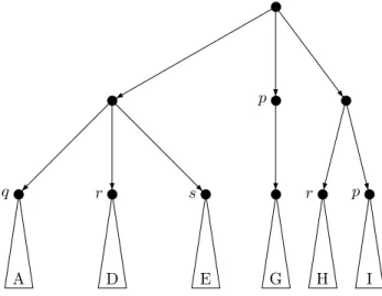
In the following, we fix a letter c ∈ Σ such that h(c) 6= 1

and we let A = Σ \ {c}. We define the c-factorization of a word v ∈ Σ

. If v ∈ (A

c)

then its c-factorization is v = v

cv

cv

c · · · with v

∈ A

for all i ≥ 0. If v ∈ (A

c)

A

then its c-factorization is v = v

cv

c · · · v

cv

where k ≥ 0 and v

∈ A

for 0 ≤ i < k and v

∈ A

.

Consider two new disjoint alphabets T

= {h(u) | u ∈ A

} and T

= {[u]

| u ∈ A

}. Let T = T

⊎ T

and define the mapping σ : Σ

→ T

by σ(v) = h(v

)h(v

)h(v

) · · · ∈ T

if v ∈ (A

c)

and its c-factorization is v = v

cv

cv

c · · · , and σ(v) = h(v

)h(v

) · · · h(v

)[v

]

∈ T

T

if v ∈ (A

c)

A

and its c-factorization is v = v

cv

c · · · v

cv

.

Lemma 8.2. Let L ⊆ Σ

be a language recognized by h. There exists a language K ⊆ T

which is definable in LTL

[ XU ] and such that L = σ

(K).

Proof. We have seen that the local divisor M

= h(c)M ∩ M h(c) is an aperiodic monoid with composition ◦ and neutral element h(c). Moreover,

|M

| < |M | since h(c) 6= 1

. Let us define a morphism g : T

→ M

as follows. For m = h(u) ∈ T

we define g(m) = h(c)mh(c) = h(cuc). For m ∈ T

we let g(m) = h(c), which is the neutral element in M

.

Let K

= {[u]

| u ∈ L ∩ A

} ⊆ T

. We claim that L ∩ A

= σ

(K

).

One inclusion is clear. Conversely, let v ∈ σ

(K

). There exists u ∈ L∩A

such that σ(v) = [u]

∈ T

. By definition of σ, this implies v ∈ A

and v ≈

u. Since u ∈ L and L is recognized by h, we get v ∈ L as desired.

For n ∈ T

and m ∈ T

, let K

= nT

m ∩ n[n

σ(L) ∩ T

m]

and let K

= S

n∈T1,m∈T2

K

. We claim that L ∩ (A

c)

A

= σ

(K

).

Let first v ∈ L ∩ (A

c)

A

and write v = v

cv

· · · cv

its c-factorization.

With n = h(v

) and m = [v

]

we get σ(v) ∈ K

. Conversely, let

v ∈ σ

(K

) with n ∈ T

and m ∈ T

. We have v ∈ (A

c)

A

and

its c-factorization is v = v

cv

· · · cv

with k > 0, h(v

) = n and [v

]

=

m. Moreover, x = h(v

) · · · h(v

)[v

]

∈ [n

σ(L) ∩ T

m]

hence we

find y ∈ T

m with g(x) = g(y) and ny ∈ σ(L). Let u ∈ L be such

that σ(u) = ny ∈ nT

m. Then u ∈ (A

c)

A

and its c-factorization is u = u

cu

· · · cu

with ℓ > 0, h(u

) = n and [u

]

= m. By definition of g, we get h(cv

c · · · cv

c) = g(x) = g(y) = h(cu

c · · · cu

c). Using h(v

) = n = h(u

) and [v

]

= m = [u

]

, we deduce that v ≈

u. Since u ∈ L and L is recognized by h, we get v ∈ L as desired.

For n ∈ T

, let K

= nT

∩n[n

σ(L)∩T

]

and let K

= S

n∈T1

K

. As above, we shall show that L ∩ (A

c)

= σ

(K

). So let v ∈ L ∩ (A

c)

and consider its c-factorization v = v

cv

cv

· · · . With n = h(v

), we get σ(v) ∈ K

. To prove the converse inclusion we need some auxiliary results.

First, if x ∼

y ∼

z with x ∈ T

and |y|

< ω then x ∼

z. Indeed, in this case, we find factorizations x = x

x

x

· · · and y = y

y

y

· · · with x

∈ T

, y

∈ T

and y

∈ T

for i > 0 such that g(x

) = g(y

) for all i ≥ 0. Similarly, we find factorizations z = z

z

z

· · · and y = y

y

y

· · · with z

∈ T

, y

∈ T

and y

∈ T

for i > 0 such that g(z

) = g(y

) for all i ≥ 0. Then, we have g(x

) = g(y

) = h(c) = g(y

) = g(z

) for all i > 0 and g(x

) = g(y

) = g(y

) = g(z

) since y

and y

contain all letters of y from T

and g maps all letters from T

to the neutral element of M

.

Second, if x ∼

y ∼

z with |y|

= ω then x ∼

y

∼

z for some y

∈ T

. Indeed, in this case, we find factorizations x = x

x

x

· · · and y = y

y

y

· · · with x

∈ T

, and y

∈ T

T

T

such that g(x

) = g(y

) for all i ≥ 0. Let y

be the projection of y

to the subalphabet T

and let y

= y

y

y

· · · ∈ T

. We have g(y

) = g(y

), hence x ∼

y

. Similarly, we get y

∼

z.

Third, if σ(u) ∼

σ(v) with u, v ∈ (A

c)

then cu ≈

cv. Indeed, since u, v ∈ (A

c)

, the c-factorizations of u and v are of the form u

cu

c · · · and v

cv

c · · · with u

, v

∈ A

. Using σ(u) ∼

σ(v), we find new factorizations u = u

cu

c · · · and v = v

cv

c · · · with u

, v

∈ (A

c)

A

and h(cu

c) = h(cv

c) for all i > 0. We deduce

cu = (cu

c)u

(cu

c)u

· · · ∼

(cv

c)u

(cv

c)u

· · · = cv

(cu

c)v

(cu

c) · · ·

∼

cv

(cv

c)v

(cv

c) · · · = cv.

We come back to the proof of σ

(K

) ⊆ L ∩ (A

c)

. So let u ∈ σ

(K

). We have u ∈ (A

c)

and σ(u) = nx ∈ nT

with x ∈ [n

σ(L)∩

T

]

. Let y ∈ T

be such that x ≈

y and ny ∈ σ(L). Let v ∈ L with σ(v) = ny. We may write u = u

cu

and v = v

cv

with u

, v

∈ A

, h(u

) = n = h(v

), u

, v

∈ (A

c)

, x = σ(u

) and y = σ(v

). Since x ≈

y, using the first two auxiliary results above and the fact that the mapping σ : (A

c)

→ T

is surjective, we get σ(u

) ∼

σ(w

) ∼

· · · ∼

σ(w

) ∼

σ(v

) for some w

, . . . , w

∈ (A

c)

. From the third auxiliary result, we get cu

≈

cv

. Hence, using h(u

) = h(v

), we obtain u = u

cu

≈

v

cv

= v.

Since v ∈ L and L is recognized by h, we get u ∈ L as desired.

Finally, let K = K

∪ K

∪ K

. We have already seen that L = σ

(K).

It remains to show that K is definable in LTL

[ XU ]. Let N ⊆ T

, then, by definition, the language [N ]

is recognized by g which is a mor- phism to the aperiodic monoid M

with |M

| < |M |. By induction on the size of the monoid, we deduce that for all n ∈ T

and N ⊆ T

there exists ϕ ∈ LTL

[ XU ] such that [N]

= L

(ϕ). We easily check that nL

(ϕ) = L

(n ∧ ϕ). Therefore, the language n[N]

is definable in LTL

[ XU ]. Moreover, K

, nT

m and nT

are obviously definable in LTL

[ XU ]. Therefore, K is definable in LTL

[ XU ].

Let b ∈ Σ be a letter. For a nonempty word v = a

a

a

· · · ∈ Σ

\ {ε}

and a position 0 ≤ i < |v|, we denote by µ

(v, i) the largest factor of v starting at position i and not containing the letter b except maybe a

. Formally, µ

(v, i) = a

a

· · · a

where ℓ = max{k | i ≤ k < |v| and a

6=

b for all i < j ≤ k}.

Lemma 8.3 (Lifting) . For each formula ϕ ∈ LTL

[ XU ], there exists a formula ϕ

∈ LTL

[ XU ] such that for each v ∈ Σ

\{ε} and each 0 ≤ i < |v|, we have v, i | = ϕ

if and only if µ

(v, i), 0 | = ϕ.

Proof. The construction is by structural induction on ϕ. We let a

= a.

Then, we have ¬ϕ

= ¬ϕ

and ϕ ∨ ψ

= ϕ

∨ ψ

as usual. For next-until, we define ϕ XU ψ

= (¬b ∧ ϕ

) XU (¬b ∧ ψ

).

Assume that v, i | = ϕ XU ψ

. We find i < k < |v| such that v, k | = ¬b∧ψ

and v, j | = ¬b ∧ ϕ

for all i < j < k. We deduce that µ

(v, i) = a

a

· · · a

with ℓ > k and that µ

(v, i), k − i | = ψ and µ

(v, i), j − i | = ϕ for all i < j < k. Therefore, µ

(v, i), 0 | = ϕ XU ψ as desired. The converse can be

shown similarly.

Lemma 8.4. For all ξ ∈ LTL

[ XU ], there exists a formula ξ e ∈ LTL

[ XU ] such that for all v ∈ Σ

we have cv, 0 | = ξ e if and only if σ(v), 0 | = ξ.

Proof. The proof is by structural induction on ξ. The difficult cases are for the constants m ∈ T

or m ∈ T

.

Assume first that ξ = m ∈ T

. We have σ(v), 0 | = m if and only if v = ucv

with u ∈ A

∩ h

(m). The language A

∩ h

(m) is recognized by the restriction h

: A

→ M . By induction on the size of the alphabet, we find a formula ϕ

∈ LTL

[ XU ] such that L

(ϕ

) = A

∩ h

(m). We let

e

m = ϕ

∧ XF c. By Lemma 8.3, we have cv, 0 | = m e if and only if v = ucv

with u ∈ A

and µ

(cv, 0), 0 | = ϕ

. Since µ

(cv, 0) = cu, we deduce that cv, 0 | = m e if and only if v = ucv

with u ∈ L

(ϕ

) = A

∩ h

(m).

Next, assume that ξ = m ∈ T

. We have σ(v) | = m if and only if

v ∈ A

∩ m (note that letters from T

can also be seen as equivalence

classes which are subsets of Σ

). The language A

∩ m is recognized by

the restriction h

. By induction on the size of the alphabet, we find a formula ψ

∈ LTL

[ XU ] such that L

(ψ

) = A

∩ m. Then, we let

e m = ψ

c

∧ ¬ XF c and we conclude as above.

Finally, we let ¬ξ f = ¬ ξ, e ξ ^

∨ ξ

= ξ e

∨ ξ e

and for the modality next-until we define ξ

^ XU ξ

= (¬c ∨ ξ e

) U (c ∧ ξ e

).

Assume that σ(v), 0 | = ξ

XU ξ

and let 0 < k < |σ(v)| be such that σ(v), k | = ξ

and σ(v), j | = ξ

for all 0 < j < k. Let v

cv

cv

c · · · be the c-factorization of v. Since the logics LTL

[ XU ] and LTL

[ XU ] are pure future, we have σ(v), k | = ξ

if and only if σ(v

cv

· · · ), 0 | = ξ

if and only if (by induction) cv

cv

· · · , 0 | = ξ e

if and only if cv, |cv

· · · cv

| | = ξ e

. Similarly, σ(v), j | = ξ

if and only if cv, |cv

· · · cv

| | = ξ e

. Therefore, cv, 0 | = ξ

^ XU ξ

. The converse can be shown similarly.

We conclude now the proof of Proposition 8.1. We start with a language L ⊆ Σ

recognized by h. By Lemma 8.2, we find a formula ξ ∈ LTL

[ XU ] such that L = σ

(L

(ξ)). Let ξ e be the formula given by Lemma 8.4.

We claim that L = L

( ξ). Indeed, for e v ∈ Σ

, we have v ∈ L

( ξ) if e and only if cv, 0 | = ξ e if and only if (Lemma 8.4) σ(v), 0 | = ξ if and only if σ(v) ∈ L

(ξ) if and only if v ∈ σ

(L

(ξ)) = L.

9 The separation theorem

As seen in Section 7, an LTL

[ YS , XU ] formula ϕ can be viewed as a first- order formula with one free variable. The converse, in a stronger form, is established in this section.

Proposition 9.1. For all first-order formulae ξ in one free variable we find a finite list (K

, a

, L

)

where each K

∈ SF(Σ

) and each L

∈ SF(Σ

) and a

is a letter such that for all u ∈ Σ

, a ∈ Σ and v ∈ Σ

we have

(uav, |u|) | = ξ if and only if u ∈ K

, a = a

and v ∈ L

for some 1 ≤ i ≤ n.

Proof. By Proposition 4.2, with V = {x} we have [[ξ]]

∈ SF(Σ

). Hence, we can use Lemma 3.2 with A = Σ

and B = Σ

. Note that N

= B

AB

. Hence, we obtain

[[ξ]]

= [

i=1,...,n

K

· a

· L

with a

∈ A, K

∈ SF (B

) and L

∈ SF (B

) for all i. Let π : B

→ Σ

be

the bijective renaming defined by π(a, τ) = a. Star-free sets are preserved

by injective renamings. Hence, we can choose K

= π(K

) ∈ SF(Σ

) and

L

= π(L

) ∈ SF(Σ

). Note also that a

= (a

, 1) for some a

∈ Σ.

Theorem 9.2 (Separation). Let ξ(x) ∈ FO

(<) be a first-order formula with one free variable x. Then, ξ(x) = ζ(x) for some LTL formula ζ ∈ LTL

[ YS , XU ]. Moreover, we can choose for ζ a disjunction of conjunctions of pure past and pure future formulae:

ζ = _

1≤i≤n

ψ

∧ a

∧ ϕ

where ψ

∈ LTL

[ YS ], a

∈ Σ and ϕ

∈ LTL

[ XU ]. In particular, every first-order formula with one free variable is equivalent to some formula in FO

.

Note that we have already established a weaker version which applies to first-order sentences. Indeed, if ξ is a first-order sentence, then L(ϕ) is star-free by Proposition 10.3, hence aperiodic by Proposition 6.2, and finally definable in LTL by Proposition 8.1. The extension to first-order formulae with one free variable will also use the previous results.

Proof. By Proposition 9.1 we find for each ξ a finite list (K

, a

, L

)

where each K

∈ SF(Σ

) and each L

∈ SF(Σ

) and a

is a letter such that for all u ∈ Σ

, a ∈ Σ and v ∈ Σ

we have

(uav, |u|) | = ξ if and only if u ∈ K

, a = a

and v ∈ L

for some 1 ≤ i ≤ n.

For a finite word b

· · · b

where b

are letters we let ←−−−−−

b

· · · b

= b

· · · b

. This means we read words from right to left. For a language K ⊆ Σ

we let ← −

K = {← w − | w ∈ K}. Clearly, each ← −

K

is star-free. Therefore, using Propositions 6.2 and 8.1, for each 1 ≤ i ≤ n we find ψ b

and ϕ

∈ LTL

[ XU ] such that L

( ψ b

) = ← −

K

and L

(ϕ

) = L

. Replacing all operators XU by YS we can transform ψ b

∈ LTL

[ XU ] into a formula ψ

∈ LTL

[ YS ] such that (a ← w , − 0) | = ψ b

if and only if (wa, |w|) | = ψ

for all wa ∈ Σ

. In particular, K

= {w ∈ Σ

| wa

, |w| | = ψ

}.

It remains to show that ξ(x) = ζ(x) where ζ = W

1≤i≤n

ψ

∧ a

∧ ϕ

. Let w ∈ Σ

\ {ε} and p be a position in w.

Assume first that (w, p) | = ξ(x) and write w = uav with |u| = p. We have u ∈ K

, a = a

and v ∈ L

for some 1 ≤ i ≤ n. We deduce that ua

, |u| | = ψ

and a

v, 0 | = ϕ

. Since ψ

is pure past and ϕ

is pure future, we deduce that ua

v, |u| | = ψ

∧ a

∧ ϕ

. Hence we get w, p | = ζ.

Conversely, assume that w, p | = ψ

∧ a

∧ ϕ

for some i. As above, we write w = ua

v with |u| = p. Since ψ

is pure past and ϕ

is pure future, we deduce that ua

, |u| | = ψ

and a

v, 0 | = ϕ

. Therefore, u ∈ K

and v ∈ L

.

We deduce that (w, p) | = ξ(x).

10 Variations

This section provides an alternative way to establish the bridge from first- order to star freeness and an alternative proof for Theorem 9.2.

There is a powerful tool to reason about first-oder definable languages which we did not discuss: Ehrenfeucht-Fra¨ıss´e-games. These games lead to an immediate proof of a congruence lemma, which is given in Lemma 10.2 below. On the other hand, in our context, it would be the only place where we could use the power of Ehrenfeucht-Fra¨ıss´e-games, therefore we skip this notion and we use Lemma 10.1 instead.

Before we continue we introduce a few more notations. The quantifier depth qd(ϕ) of a formula ϕ is defined inductively. For the atomic formulae

⊥, P , and x < y it is zero, the use of the logical connectives does not increase it, it is the maximum over the operands, but adding a quantifier in front increases the quantifier depth by one. For example, the following formula in one free variable y has quantifier depth two:

∀x (∃y P (x) ∧ ¬P (y)) ∨ (∃z P (z) ∧ (x < z ) ∨ (z < y))

By FO

we mean the set of all formulae of quantifier depth at most m and where the free variables are in the set {x

, . . . , x

}, and FO

is a short-hand of FO

; it is the set of sentences of quantifier-depth at most m.

We say that formulae ϕ, ψ ∈ FO

are equivalent if L(ϕ) = L(ψ) (for all Σ). Since the set of unary predicates is finite, there are, up to equivalence, only finitely many formulae in FO

as soon as k and m are fixed. This is true for m = 0, because over any finite set of formulae there are, up to equivalence, only finitely many Boolean combinations. For m > 0 we have, by induction, only finitely many formulae of type ∃x

ϕ where ϕ ranges over FO

. A formula in FO

is a Boolean combination over such formulae, as argued for m = 0 there are only finitely many choices.

10.1 The congruence lemma

Recall that Σ

means the set of pairs (w, p), where w ∈ Σ

is a finite or infinite word and p = (p

, . . . , p

) is a k-tuple of positions in pos(w). If we have (u, p) ∈ Σ

and (v, q) ∈ Σ

, then we can define the concatenation in the natural way by shifting q:

(u, p) · (v, q) = (uv, p

, . . . , p

, |u| + q

, . . . , |u| + q

) ∈ Σ

. For each k and m and (w, p) ∈ Σ

we define classes as follows:

[(w, p)]

= \

ϕ∈FOm,k|(w,p)|=ϕ

L(ϕ).