Riemann Solver
Problem sheet 7/8 16/06/2009, 23/06/2009
We have seen that the exact Riemann solver is an expensive method and in more general case, such as MHD equations, Riemann invariants are actually very dicult to acquire.
Problem sheet 7/8 is a series of problems that help to develop a 1D HLL-type Riemann solver that is practically useful and can be easily extended to solve multi-dimensional equations. Here is the plan:
1. We rst solve the jump condition and Riemann invariants for isothermal equation.
2. We derive and develop Riemann solver based on HLL.
3. We solve a Riemann problem numerically and compare the results with the exactly solution from 1. Here, we are not trying to really overlap the exact solution on the numerical results. But we do know the values and speeds of the breaking points which divide the wave structures into dierent regions.
4. Implement the higher order scheme based on MUSCL-Hancock method.
1 Riemann problem (analytic part)
We are going to solve the following hydrodynamic equation ρ
ρu
t
+
ρu ρu2+c2sρ
x
= 0. (1)
Assuming the state vector,q, and ux vector,f,
qt+∂f
∂qqx= 0, (2)
with ∂∂qf being the Jacobian matrix as a function of state vector.
1. Find the two eigenvaluesλ1< λ2 and the corresponding eigenvectorse1, e2.
2. Apply the Rankine-Hugoniot jump condition to the two characteristic fam- ilies. Derive the following relations:
ul=ur±cs( rρl
ρr − rρr
ρl), (3)
with '+' corresponds to the 1-shock and '−' the 2-shock. Jump condition tells us how the state vector changes in the shock discontinuity.
3. Since the solution is self-similar, with the auxiliary variableξ =x/t, eq.
(2) reads
∂f
∂qq0(ξ)=ξq0(ξ). (4) It shows thatq0(ξ)∝e1,2 andξrepresents the corresponding eigenvalues.
Eq. (4) tells us how the state vector changes in the smooth region(if it is a simple wave). Solve the following dierential equation and obtain the Riemann invariants for the two characteristic famalies.
q0(ξ)=e1,2. It should look like
(ul+cslnρl=ur+cslnρr 1-rarefaction
ul−cslnρl=ur−cslnρr 2-rarefaction (5)
t
qL qR x
L
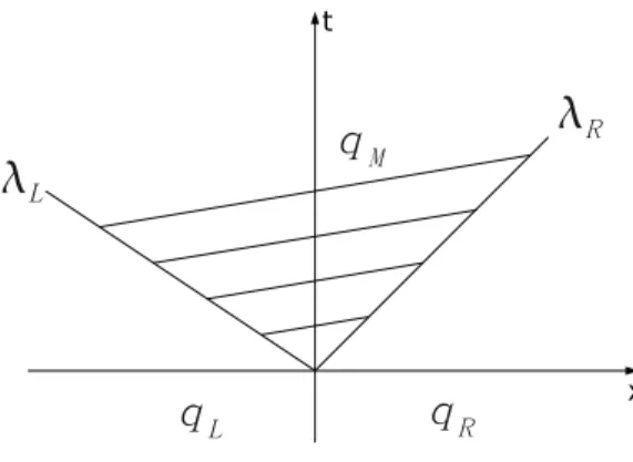
R qM
Figure 1: 2-wave HLL solver
2 HLL Solver
H(arten)-L(ax)-van L(eer) Riemann solver is a 2-wave solver and can be applied either to hydrodynamic or MHD equations. One retains only the 2 'fastest' waves (e.g. in general, the 2 fast magneto-acoustic waves) and then assume that between the 2 waves there is a uniform stateqMas shown in Fig. 1.
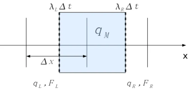
To obtain the middle stateqM, let us consider a volume of controlV, i.e. an area of surfaceS in yzand delimited by−∆xand∆xinxas shown in Fig. 2.
1. att= 0, calculate averaged value ofq(0)withinV.
2. at t = ∆t, the left and the right waves have reached: x = λL∆t and x=λR∆t. Calculateq(∆t).
3. We also have the relation
x qL,FL qR,FR
Lt
qM
Rt
x
Figure 2: Waves in volume of control.
4. Assuming thatλL<0 andλR>0(as in Fig. 2), let us consider the vol- ume of control delimited byx=−∆xand x= 0. Based on conservation law in the volume of control, prove that
FM =FL+λL(qM−qL) =λRFL−λLFR+λLλR(qR−qL)
λR−λL .
Note that this expression is symmetrical inR↔Lshowing that we will get the same result if we consider the volume of control delimited byx= ∆x andx= 0.
5. Now the ux,FHLL, at the interface can be evaluated by
FHLL=
FL λL>0, λR>0 FM λL<0, λR>0 FR λL<0, λR<0
6. The nal thing we need to decide is the value ofλLandλR. Let us follow the estimate proposed by Davis(1988):
λL= min[λ1(qL), λ1(qR)]
λR= max[λ2(qL), λ2(qR)].
7. Implement a 1D hydrodynamic code based on HLL.
3 Riemann problem (numerical part)
Consider a Riemann problem bounded by x = [0,1] with outow boundary condition:
q=
((1,0) x≤0.5 (0.125,0) x >0.5.
1. Use the code just developed to evolve this Riemann problem, run till t= 0.15.
2. Compare the numerical qM with the analytic solution. Hint: The wave structure is 1-rarefaction and 2-shock. Combine Eq.(3) and Eq.(5) to evaluate the analyticqM.
3. Are the wave speeds correct in the numerical result?
4 Higher Order scheme MUSCL-Hancock
Apply MUSCL-Hancock method to the new code with whatever slope limiter you like. Solve the Riemann problem again and compare the result with the rst order scheme.