Abstract Interpretation from B ¨uchi Automata

(1)

Abstract Interpretation from B ¨uchi Automata

Martin Hofmann

LMU Munich, Germany

martin.hofmann@ifi.lmu.de

Wei Chen

University of Edinburgh, UK

wchen2@inf.ed.ac.uk

Abstract

We describe the construction of an abstract lattice from a given Buchi automata. The abstract lattice is finite and has the following key properties. (i) There is a Galois connection between it and the (infinite) lattice of languages of finite and infinite words over a given alphabet. (ii) The abstraction is faithful with respect to acceptance by the automaton. (iii) Least fixpoints and ω-iterations (but not in general greatest fixpoints) can be computed on the level of the abstract lattice.

This allows one to develop an abstract interpretation capable of checking whether finite and infinite traces of a (recursive) program are accepted by a policy automaton. It is also possible to cast this analysis in form of a type and effect system with the effects being elements of the abstract lattice.

While the resulting decidability and complexity results are known (regular model checking for pushdown systems) the abstract lattice provides a new point of view and enables smooth integration with data types, objects, higher-order functions which are best handled with abstract interpretation or type systems.

We demonstrate this by generalising our type-and-effect systems to object-oriented programs and higher-order functions.

Categories and Subject Descriptors

Theory of computation [Se- mantics and reasoning]: Program reasoning

Keywords

Type Systems, Type-and-Effect Systems, Temporal Properties, Liveness

1. Introduction

A great range of techniques and tools have been developed and studied for the prediction of program behaviours without actually running the program [8, 10, 11, 13, 25, 27]. One of them, originat- ing from type inference in functional programming languages, is the type and effect discipline [24]. As a refinement of type systems in programming languages, types are annotated with information characterizing dynamic behaviours of programs—effects. As a result, a well-typed program satisfies some properties regarding its side-effects as well. This type-based technique has been used for all kinds of static analysis of programs, e.g. flow analysis [26], de- pendency analysis [1], resource allocation analysis [33], and amor- tised analysis [19, 20], etc. In particular, a type and effect system

Permission to make digital or hard copies of all or part of this work for personal or classroom use is granted without fee provided that copies are not made or distributed for profit or commercial advantage and that copies bear this notice and the full citation on the first page. Copyrights for components of this work owned by others than ACM must be honored. Abstracting with credit is permitted. To copy otherwise, or republish, to post on servers or to redistribute to lists, requires prior specific permission and/or a fee. Request permissions from permissions@acm.org.

CSL-LICS 2014, July 14–18, 2014, Vienna, Austria.

Copyright c2014 ACM 978-1-4503-2886-9. . . $15.00.

http://dx.doi.org/10.1145/2603088.2603127

was developed by Grabowski et al. [16] to verify that a particular programming guideline for secure web-programming has been adhered to. Generalizing from this, one could model a programming guideline as a property of traces that a program might have, where traces are sequences of events that are issued by a certain instrumentation of the program with special event-issuing operations.

This instrumentation would be part of the formalised guideline. A finite state machine would then be used to specify the set of accept- able traces. Most policies involve safety properties which can be assessed by examining finite portions of traces. In some cases, however, properties pertaining to liveness and fairness [3] can become relevant. For instance, a guideline could be that calls to appropriate logging functions must be made again and again or that event han- dlers should not become stuck, e.g. in the Java Swing framework.

This motivated us to investigate the possibility of using type systems in this situation as well. Our aim is not to offer new algorithms for deciding certain temporal properties or indeed to compete with the existing methods which are numerous [5, 8, 13, 25], but to extend the reach of type systems. Our solution goes, however, beyond a simple reformulation of an existing algorithm;

the abstract domain based B¨uchi automata may well be useful in its on right and is an original contribution of this work.

For the sake of simplicity, we introduce and study a small language consisting of recursive first-order procedures and nondeterministic choices. The language explicitly allows infinite recursions. In this language, except for primitive procedures which have events as arguments, other procedures have no inputs.

We remark that in essence our language is the same as the pushdown systems that have been studied in detail by a number of authors [5, 29, 35].

Once a satisfactory type system for such a simple language has been found, it can be combined with known techniques [4, 28]

to scale to a type system for a large fragment of Java or similar languages. Alternatively, one can use our simple language as a target of a preliminary abstraction step.

Then, we develop the B¨uchi type and effect system to capture correctly finite and infinite traces. Since branching is nondeterministic in our language, we can even establish a completeness result. Completeness, of course, will be lost, once we re-introduce data-dependent branching.

As a demonstration, we extend the B¨uchi type and effect system for this small language to a B¨uchi type and effect system for Featherweight Java with field update [4].

The main technical contribution of this paper is the design of an abstract domain in the sense of abstract interpretation [10, 11] based on B¨uchi automata or rather a mild extension of those allowing infinite as well as finite words. The proofs of soundness and completeness of the type system are based on clear-cut lattice- theoretic properties of this abstraction.

As in the finitary case, this B¨uchi abstraction is based on equiv-

alence relations on finite words generated by the policy B¨uchi au-

tomaton. Abstracted effects are no longer sets of such equivalence

(2)

classes, but rather sets of pairs of the form (U, V ) with U , V classes and representing the infinitary language U V

^ω

. While such pairs appear in B¨uchi’s original complementation construction for B¨uchi automata [6] and have subsequently been used by a number of authors [12, 17, 30], they have never been used in the context of type systems and abstract interpretation.

1.1 Related work

As already mentioned, our language of parameterless procedures is equivalent to pushdown systems for which model-checking of temporal properties has been extensively studied [7, 15, 29, 35]. Push- down systems, on the other hand, are special cases of higher-order recursion systems introduced by Knapik et al. [22] and extensively studied by Ong and his collaborators, e.g. [2, 23].

The latter work [23] also casts model checking into the form of a type system. More precisely, from an alternating parity automaton a type system for higher-order recursion schemes is derived such that a scheme is typable iff its evaluation tree would be accepted by the automaton. In this way, in particular all mu-calculus definable properties of the evaluation tree become expressible. Regarding trace languages as opposed to tree properties alternating parity automata are equivalent to B¨uchi automata since both capture the (ω−)regular languages. Thus for the trace language of interest here the system from loc.cit. is equal in expressive power to our type system. Moreover, B¨uchi automata are a well-established means for formulating specifications.

The difference is that Kobayashi and Ong’s system has a much more semantic flavour not unlike the intersection type systems used to characterise strong normalisation. More concretely, the well- formedness condition for recursions in that system requires the solution of a parity game whose size is proportional to the size of the program (number of function symbols to be precise) which is known to be equivalent to model checking trees against mu- calculus formulas.

Our type system, on the other hand, deviates from the standard type systems used in programming and program analysis only very slightly; instead of the usual recursion rule (which is clearly unsound in the context of liveness) we use a rule involving a type variable. No further semantic conditions need to be checked once of course the given B¨uchi automaton has been analysed and preprocessed. Even though the types of [23] are also based on possible transitions of a word through the automaton there are important differences, most notably the closure operation we use and the precise analysis of ω-iteration using the Ramsey theorem.

These two together allow us to precompute a finite abstract lattice that faithfully represents the concrete lattice of ≤ ω-languages. The analysis of recursive functions, whether mutual or not, thus reduces to a standard fixpoint iteration in an abstract lattice known from abstract interpretation.

Another recent work on the use of types for properties of infinite traces is [21] which embeds formulas of Linear Temporal Logic into types in the context of functional reactive programming. This work, however, relies on an encoding of linear temporal logic in first-order logic with integers, e.g., one models “the event x occurs infinitely often” as a formula like ∀i∃j.x

j

where x

j

refers to that the event x issues at the time j. Dependent types are being used to turn this into a type system, but questions of inference and decidability are not considered.

Finally, we mention the work by Skalka and his coauthors which furnish type-based translations of higher-order [31] and object- oriented [32] to pushdown systems. The so obtained pushdown systems can then be fed into off-the-shelf model-checking algorithms.

The difference to our approach is that types do not contain the full information about the possible traces but only a finite abstraction which is just fine enough to decide compliance with a

given policy. In this way, one may expect more succinct types, more efficient inference, and better interaction with the user. Another difference is that our approach is entirely based on type systems and abstract interpretation and as such does not rely on external model-checking software. This might make it easier to integrate our approach with certification. One can also argue that our approach is more in line with classical type and effect systems where types do not contain programs either but rather succinct abstractions akin to our effects.

2. Preliminaries

Let Σ be a finite alphabet. We write Σ

^∗

for the set of finite words over Σ, we write Σ

^≤ω

for the set of finite and infinite words, and Σ

^ω

for the set of infinite words. Finite words can be concatenated with finite or infinite words as usual and this extends to languages.

We assume that programs are instrumented with special commands issuing events from Σ. In this way, we can associate with each execution of a(n) (instrumented) program P a trace which is a word from Σ

^≤ω

. Terminating executions have finite traces (in Σ

^∗

) whereas nonterminating executions may have finite or infinite traces.

We also assume a language L

0

⊆ Σ

^≤ω

of finite and infinite traces modelling the allowed traces. This language L

0

will be represented by a finite state automaton

A—the policy automa-

ton. Writing L(P ) for the language of possible (finite and infinite) traces and L

0

= L(A) for the policy language we thus are interested in determining whether or not L(P ) ⊆ L(A). While of course such questions are in general undecidable it becomes tractable if branches in the control flow of P are overapproximated by non-determinism or at least only depend on an appropriate finite abstraction of the data relevant in the branching conditions.

We remark that the expressive power of B¨uchi automata strictly subsumes the linear time mu-calculus and equals that of monadic second-order logic.

We now define a finite lattice

M

and functions γ :

M

→ P (Σ

^≤ω

) α : P(Σ

^≤ω

) →

M

forming a Galois connection (Theorem 2(2)).

The abstraction is faithful with respect to containment in the language of the policy automaton in the sense that γ(α(L(A))) = L(A) and hence L ⊆ L(A) iff α(L) ⊆ α(L(A)) (Theorem 2(5)).

On the other hand, various language-theoretic operations can be represented faithfully on the level of the abstraction, in particular, union, concatenation, least fixpoints and ω-iteration. These will allow us to design a type system that computes the abstraction α(L(P)) of a program’s behaviour.

For the most part, existence of these abstract operations follows from the Galois connection; in particular, if α ◦ F = F

α

◦ α then α(lfp(F )) = lfp(F

α

), where lfp denotes the least fixpoint, F

α

is the corresponding abstraction function of F and ◦ denotes functional composition. A nontrivial property of our particular abstraction that does not follow from general lattice-theoretic considera- tions is the fact that ω-iteration can be faithfully represented on the level of the abstractions: There is an operation (−)

^(ω)

:

M∗

→

M

(with

M∗

denoting the sublattice containing abstractions of languages of finite words) satisfying α(L

^ω

) = α(L)

^(ω)

(Theorem 4).

This then allows us to represent all the language-theoretic op-

erations arising in the construction of L(P ) on the level of the

abstraction. Therefore, we can describe the behaviour of program

parts directly with the abstractions of their behaviours—the ab-

stractions become effects in a type-and-effect system or can be used

for abstract interpretation directly.

(3)

3. Extended B ¨uchi automata

We define a mild generalization of B¨uchi automata which is capable of describing languages of both finite and infinite words.

Definition 1.

An extended B¨uchi Automaton is a quintuple

A

= (Q, Σ, δ, q

0

, F ) where Q is a finite set of states, Σ is an alphabet;

hereafter always required to be equal to the fixed alphabet of events; δ : Q × Σ → P (Q) the transition function, the initial state q

0

∈ Q, and the set F ⊆ Q of final states. The language L(A) of

A

is defined as: the set of all finite words by which a final state can be reached from the initial state and all infinite words admitting an infinite run (in the usual sense) which starts from the initial state and goes through final states infinitely often. Thus, L(A) is the union of

A’s language when understood as a traditional NFA and

its language when understood as a traditional B¨uchi automaton.

Note that if an extended B¨uchi automaton accepts an infinite word then it will also accept infinitely many prefixes of that word.

This means that these automata cannot accept all unions of regular and ω-regular languages.

Our philosophy is that an actually terminating trace could, if so desired, marked by issuing a special end event, say $. The finite traces not ending in $ and thus stemming from an idling computation should be understood as infinite traces which from some point on consist exclusively of invisible stuttering events, say

X

. Assuming further that each state has an implicit self-loop labelled

X

our acceptance condition for those words is subsumed by the usual B¨uchi condition. The following theorem summarises this.

Theorem 1.

Let L

1

⊆ Σ

^∗

be a regular language over Σ and L

2

⊆ (Σ ∪ {X})

^ω

be an ω-regular language. Suppose furthermore that whenever w ∈ L

1

and w

⁰

arises from w by inserting

X

symbols in arbitrary positions, then w

⁰

∈ L

2

(Of course, L

2

may contain words other than those enforced by this clause). There is an extended B¨uchi automaton that accepts the language L

1

$ ∪ L

^X2

where L

^X₂

⊆ Σ

^≤ω

comprises all finite and infinite words that can be obtained from words in L

2

by deleting all

X

-symbols.

Proof. Start with a B¨uchi automaton for L

2

and replace all

X

- edges with -edges. This automaton viewed as an extended B¨uchi automaton then accepts L

^X2

. Form a disjoint union with an NFA for L

1

$ which has the additional property that no final state has an outgoing edge so that no spurious infininite words get accepted accidentally.

3.1 Equivalence classes

Following B¨uchi’s original work we consider equivalence relations on finite words induced by an extended B¨uchi automaton.

We write q

^w

q

⁰

to mean that the state q

⁰

is reachable from state q by using the finite word w. Furthermore, q

^wF

q

⁰

denotes that by using the finite word w, the state q

⁰

can be reached from the state q in such a way that a final state is visited on the way. In particular, q

^w

q

⁰

with q ∈ F or q

⁰

∈ F implies q

^wF

q

⁰

. Formally, we have q

^wF

q

⁰

iff there exists q

⁰⁰

∈ F and u, v such that w = uv and q

^u

q

⁰⁰

and q

⁰⁰ ^v

q

⁰

.

For nonempty words w, u ∈ Σ

⁺

we define w ∼ u as:

∀p, q ∈ Q . p

^w

q ⇔ p

^u

q ∧ p

^wF

q ⇔ p

^uF

q . We then extend ∼ to an equivalence relation on Σ

^∗

by adding ∼ . No nonempty word is equivalent to . We write [w] for the equivalence class of w ∈ Σ

^∗

. Note that the quotient set Σ

^∗

/∼

contains the ∼-equivalence classes consisting of nonempty words and the special class [] = {}.

We can effectively represent a class [w] by the two relations on states it induces, i.e., by {(q, q

⁰

) | q

^w

q

⁰

} and {(q, q

⁰

) | q

^wF

q

⁰

}. Note that these relations are independent of the choice of the representative w. This also implies an upper bound on the number of classes and a fortiori that there are finitely many.

Lemma 1.

If n is the number of states of the policy automaton inducing ∼, then Σ

^∗

/∼ has at most 2

²ⁿ²

+ 1 elements.

We notice that if w ∼ u and w

⁰

∼ u

⁰

then ww

⁰

∼ uu

⁰

. As a result, concatenation is well-defined on equivalence classes. Thus, Σ

⁺

/ ∼ becomes a semigroup and Σ

^∗

/ ∼ a monoid.

Notice, however, that monoid multiplication is not in general the same as concatenation of languages. We have [u][v] = [uv]

by definition and if x ∈ [u], y ∈ [v] then xy ∈ [uv], but if xy ∈ [uv] it need not be the case that x ∈ [u] and y ∈ [v]. On the other hand, the language-theoretic concatenation of [u] and [v]

is contained in a (unique) class and this class is [u][v]. The operator- less juxtaposition for monoid multiplication is therefore to be used with some care, but on the other hand is vindicated by general mathematical practice.

The following Lemma is a straightforward consequence of standard results about B¨uchi automata [34].

Lemma 2.

Fix an extended B¨uchi automaton

A.

(a) The elements of Σ

^∗

/∼ are regular languages;

(b) for all C in Σ

^∗

/∼, C ∩ L(A) 6= ∅ implies C ⊆ L(A);

(c) for all C and D in Σ

^∗

/∼, CD

^ω

∩ L(A) 6= ∅ implies CD

^ω

⊆ L(A);

(d) for all w ∈ Σ

^≤ω

there exist classes C, D ∈ Σ

^∗

/∼ so that w ∈ CD

^ω

and CD = C and DD = D.

The sets CD

^ω

(with CD = C and DD = D) thus behave almost like classes themselves, but an important difference is that they may nontrivially overlap. If CD

^ω

∩ U V

^ω

6= ∅ then in general one cannot conclude CD

^ω

= U V

^ω

. We also remark that Ramsey’s theorem is used in the proof of (d). It is actually a special case of Lemma 5 below so that we do not need to recall the proof here.

Example 1.

For a concrete example, consider the following automaton:

A

: //?>=< 89:; ₀

b

^a

)) ?>=< 89:; /.-, ()*+ ₁

b

ii

a

There are four equivalence classes: [] and [a] = (a + b)

^∗

a and [b] = b

⁺

and [ab] = (a + b)

^∗

b − [b]. We have [a][a] = [b][a] = [ab][a] = [a] and [b][b] = [b] and [a][b] = [a][ab] = [b][ab] = [ab][b] = [ab][ab] = [ab]. Now (ab)

^ω

∈ [ab][ab]

^ω

∩ [a][a]

^ω

, but [ab][ab]

^ω

6= [a][a]

^ω

because a

^ω

∈ [a][a]

^ω

\ [ab][ab]

^ω

.

4. B ¨uchi Abstraction

Lemma 2 shows that given an extended B¨uchi automaton

A, with-

out affecting property checking, we can use sets of classes in Σ

^∗

/∼

to represent languages over Σ

^∗

and sets of pairs of classes (C, D) such that CD = C and DD = D to represent languages over Σ

^≤ω

.

However, it is necessary to close such sets up under overlapping

“patches”

Definition 2.

A pair (C, D) such that CD = C and DD = D is called a patch. One defines the extent of a patch (C, D) as γ(C, D) = CD

^ω

, the set of all finite and infinite words that admit a decomposition w = w

0

w

1

w

2

. . . such that w

0

∈ C and w

i

∈ D for i > 0. The extent of a set of patches V is defined by γ(V) =

S

(C,D)∈V

γ(C, D). Two patches (U, V ) and (C, D)

meet if γ(U, V ) ∩ γ(C, D) 6= ∅. A set of patches V is closed if

γ(C, D) ∩ γ(V) 6= ∅ implies (C, D) ∈ V. We define the closure V

(4)

of V as the least closed superset of V. For typographical reasons, we also write V for the closure.

Notice that since there are only finitely many patches we can effectively compute the closure by successively adding patches.

We call a patch (U, V ) finitary if V = [] thus γ(U, V ) ⊆ Σ

^∗

.

Lemma 3.

The extent of a patch contains a finite word iff it is finitary. Finitary patches only contain finite words and they do not meet unless they are equal. Sets of finitary patches are always closed.

Proof. No class other than [] contains the empty word, thus a patch (U, V ) with V 6= [] contains infinite words only. The rest is obvious.

4.1 The abstract lattice

Our abstract lattice now consists of the closed sets of patches ordered by inclusion. We thus define

M

= {V | V closed}

We also denote

M∗

the sublattice consisting of sets of finitary patches.

We define the abstraction function α : P(Σ

^≤ω

) →

M

by α(L) = {(U, V ) | γ(U, V ) ∩ L 6= ∅}

In other words, to form the abstraction α(L) of a language L we take the smallest closed set of patches whose extents cover L.

Theorem 2.

1. The set

M

ordered by inclusion is a complete lattice; the sublattice

M∗

is isomorphic to the powerset lattice P(Σ

^∗

/∼).

2. The abstraction function together with the concretisation function γ form a Galois connection between

M

and P(Σ

^≤ω

):

L ⊆ γ(V) ⇐⇒ α(L) ⊆ V

3. α(γ(V)) = V holds for all V so we have in fact a Galois insertion

4. The abstraction function preserves unions, least and greatest elements, but not in general intersections.

5. If

A

is the underlying policy automaton then L(A) = γ(α(L(A))), hence

L ⊆ L(A) ⇐⇒ α(L) ⊆ α(L(A))

Proof. Closed sets are closed under union and intersection. So the lattice-theoretic operations are inherited from the powerset lattice.

The second part is direct from Lemma 3.

For the Galois connection assume L ⊆ γ(V). To show α(L) ⊆ V it is enough to show (U, V ) ∈ V whenever (U, V ) meets L since V is closed. So suppose w ∈ γ(U, V ) and w ∈ L for some word w. By assumption, w ∈ γ(V), so w is contained in some patch (C, D) ∈ V. Thus, since V is closed, it must contain (U, V ) as well. The converse follows directly from the obvious fact L ⊆ γ(α(L)).

The fact that we have a Galois insertion, as well as preservation of least elements and unions is obvious from the definitions.

Preservation of the greatest element follows from Lemma 2(d).

The last part follows from Lemma 2(c).

Furthermore, the abstraction function preserves unions, least and greatest elements.

For a monotone operator F on a complete lattice L we denote lfp its least fixpoint. As is well-known this fixpoint is given by the formula lfp(F ) =

T

{X | F (X ) ⊆ X } where

T

and ⊆ refer to the lattice-theoretic operations.

The following is folklore and is an easy exercise in general lattice-theoretic reasoning.

Lemma 4.

Let L, M be complete lattices, α : L → M and γ : M → L form a Galois insertion, i.e., both α, γ are monotone and α(L) ⊆ M ⇐⇒ L ⊆ γ(M) and α(γ(M )) = M , then α preserves least fixpoints in the sense that if F : L → L and F

a

: M → M are monotone and such that α ◦ F = F

a

◦ α then α(lfp(F )) = lfp(F

a

).

4.2 Concatenation and iteration

We will now define some operators on the abstract domain that track language-theoretic operations on P(Σ

^≤ω

).

Definition 3.

For U ∈

M∗

and V ∈

M

we define their abstract concatenation by

U · V = ({(AC, D) | (A, []) ∈ U ∧ (C, D) ∈ V}})

Theorem 3.

1. If U ∈

M∗

and V ∈

M

then U · V ∈

M.

2. α(L

1

L

2

) = α(L

1

) · α(L

2

).

3. If both U and V are finitary so is U · V. The abstract concatenation operation is monotone.

Proof. If (AC, D)) ∈ U · V and (C, D) ∈ V then ACD = AC since CD = C.

For the second part it is easy to see from the definition and using the Galois connection that α(L

1

L

2

) ⊆ α(L

1

) · α(L

2

).

For the converse, since α(L

1

L

2

) is closed, it suffices to prove {(AC, D) | (A, []) ∈ U ∧ (C, D) ∈ V} ⊆ α(L

1

L

2

) So, assume (AC, D) ∈ α(L

1

) · α(L

2

) where (A, []) ∈ α(L

1

) and (C, D) ∈ α(L

2

). It follows that A ∩ L

1

6= ∅. If (C, D) meets L

2

then (AC, D) meets L

1

L

2

and we are done. Otherwise, we can inductively assume that (C, D) meets (C

⁰

, D

⁰

) ∈ α(L

2

) and (AC

⁰

, D

⁰

) ∈ α(L

1

L

2

) has already been shown. It then follows that (AC, D) ∈ α(L

1

L

2

) since (AC, D) meets (AC

⁰

, D

⁰

).

The third part of the lemma is direct.

We remark that since finite iteration can be defined as a least fixpoint of operations that can be tracked on the level of the abstraction it is easy to define an operator (−)

^(∗)

on

M∗

so that α(L

^∗

) = α(L)

^(∗)

holds for L ⊆ Σ

^∗

. Namely, we simply take U

^(∗)

= lfp(λX .α({}) ∪ U · X ).

The situation is different with the infinite iteration L

^ω

of a language L ⊆ Σ

^∗

. It can be expressed as a greatest fixpoint of an operator that is representable on the level of the abstraction. To wit, L

^ω

equals the greatest fixpoint of λX.(L− {}) ·X ∪ G where G = L

^∗

if ∈ L and G = ∅, otherwise.

However, the abstraction does not in general preserve greatest fixpoints. For a concrete counterexample, consider the automaton from Example 1 and let L = {a}, we have α(L) = {([a], [])} and

α(L)

^ω

= {([a], [a]), ([ab], [ab])}

Yet, the greatest fixpoint of (λX .α(L) ·X ) also contains ([ab], [b]).

Fortunately, it is possible to track infinite iteration on the level of the abstraction but this is a nontrivial result that again requires the use of the Ramsey theorem.

Definition 4.

For U ∈

M∗

we define the abstract ω-iteration by U

^(ω)

= α(γ(U)

^ω

)

It is clear that if it is at all possible to track ω-iteration then this definition works but whether it is is not yet clear. We also remark that despite its seemingly nonconstructive definition U

^(ω)

can easily be computed using, e.g. B¨uchi nonemptiness by noticing that CD

^ω

∩ U

^(ω)

is ω regular.

The required use of Ramsey’s theorem is encapsulated in the

following combinatorial lemma.

(5)

Lemma 5.

Let (L

i

)

i∈I

be a family of classes (from Σ

^∗

/∼) and put P =

Q

i∈I

L

i

⊆ Σ

^≤ω

, i.e., P comprises finite or infinite words of the form w

1

w

2

w

3

. . . where w

i

∈ L

i

for i ≥ 1. There exist classes U, V ∈ Q where U V = U, V V = V such that P ⊆ U V

^ω

. Proof. Let w ∈ P and write w = w

1

w

2

w

3

· · · w

i

· · · where w

i

∈ L

i

. If w is a finite word then there exists n such that w

i

= (and L

i

= []) for i ≥ n and we can choose U = L

1

. . . L

n−1

and V = []. Otherwise, use Ramsey’s theorem as in the proof of Lemma 2 to obtain a sequence of indices i

1

< i

2

< i

3

<

i

4

< . . . and classes U, V where V 6= [] and V V = V , U V = U such that w

1

w

2

. . . w

i₁

∈ U , w

i₁+1

. . . w

i₂

∈ V and w

i₂+1

. . . w

i₃

∈ V and so on. It follows that U = L

1

L

2

. . . L

i₁

and V = L

i_k+1

. . . L

i_k+1

for k ≥ 1 and thus P ⊆ U V

^ω

as required.

We are now in a position to assert the desired correctness of abstract ω-iteration which constitutes our main technical result.

Theorem 4.

For any L ⊆ Σ

^∗

one has α(L

^ω

) = α(L)

^(ω)

The operator (−)

^(ω)

is monotone.

Proof. The direction ⊆ is direct from the definition; for the converse assume (U, V ) ∈ α(L)

^(ω)

= α(γ(α(L))

^ω

). Since α(L

^ω

) is closed, we may without loss of generality assume that U V

^ω

∩ γ(α(L))

^ω

6= ∅. Pick w ∈ U V

^ω

∩ γ(α(L))

^ω

and decompose w = w

1

w

2

. . . where w

i

∈ γ(α(L)). Define L

i

:= [w

i

] and apply Lemma 5 to obtain U

⁰

, V

⁰

with

Q

i

L

i

⊆ U

⁰

V

^0ω

. Note that, since w ∈ P , we have U V

^ω

∩ U

⁰

V

^0ω

6= ∅.

Now, since w

i

∈ γ(α(L)), by the definition of α, we must have that L

i

∩ L 6= ∅. Choose w

⁰i

∈ L

i

∩ L. The word w

⁰1

w

⁰2

. . . is then contained in L

^ω

∩ U

⁰

V

^0ω

, so (U

⁰

, V

⁰

) ∈ α(L

^ω

) and, finally, (U, V ) ∈ α(L

^ω

) since α(L

^ω

) is closed and U V

^ω

∩ U

⁰

V

^0ω

6=

∅.

5. Applications

We begin by the definition of a type system for a simple language with recursive procedures and nondeterministic branching. It would be possible to include state and data-dependent branching, but since the type system we design is oblivious to those we refrain from doing so.

5.1 Recursive procedures

The syntax of expressions is: e ::= o(a) | f | e

1

; e

2

| e

1

? e

2

where o(a) is the only primitive procedure which generates an event a taken from a fixed alphabet Σ of events and f ranges over procedures defined by expressions. Parentheses are used to elimi- nate ambiguity. We assume that the operator ; is right-associative and has higher priority than the operator ?. As an example, we can define procedures f and g as: f = o(b) ? o(a) ; g and g = f ; g ; (o(b) ? o(a)). Formally, thus a program consists of a finite set of procedure identifiers F and for each f ∈ F an expression e

f

defining f where calls to procedures from F are allowed and in particular, f may occur recursively in e

f

.

From now on, we fix such a program P = (F , (e

f

)

f∈F

) and call an expression e well-formed if it uses calls to procedures from F only.

Since the operator ? is non-deterministic and non-primitive procedures have no arguments, stacks and heaps are not needed at this level of abstraction.

A formal semantics is given in Appendix A. Here, we merely assume that two judgments e ↓ w for w ∈ Σ

^∗

and e ↑ w for w ∈ Σ

^≤ω

have been defined with the following intended meaning. If e ↓

w holds then there exists a terminating execution of e producing the finite trace w. If e ↑ w then there exists a non-terminating execution of e producing the finite or infinite trace w. All possible executions of e are captured by these two judgments. The judgements can be defined in a variety of ways, e.g. using inductive/coinductive definitions, by translation to pushdown systems [29], or using finite approximations. For a detailed elaboration of the third option we refer to our report [18].

5.2 B ¨uchi types

A pair (U, V) where U ∈

M∗

and V ∈

M

is called a B¨uchi effect. A B¨uchi effect approximates the traces of an expression e if whenever e ↓ w then w ∈ γ(U) and if e ↑ w then w ∈ γ(V).

Intuitively, our typing judgement will derive judgements of the form ` e&(U, V) with the idea that if such judgement is derivable then (U, V) approximates e. Given this intuition, typing rules like P

RIM

, I

F

are self-explanatory if we ignore for now the (X) deco- rations. Rule S

EQ

takes the fact into account that in a sequential composition e

1

; e

2

even a finite trace of e

1

dominates if e

1

does not terminate.

In order to overcome the obstacle with recursive procedures discussed in the introduction we need to parameterise B¨uchi effects with abstractions of traces (finite or infinite) of non-terminating procedures. To this end, we introduce formal expressions of the form

[

X∈X

(A

X

· X ) ∪ B

where

X

is a finite set of variables. We use notation like V(X) for such expressions.

If η maps variables from

X

to elements from

M

and V(X) is an expression over

X

then V(η) ∈

M

denotes the value obtained by replacing a variable X with η(X ) and evaluating.

We extend concatenation and union to these formal expressions in the obvious way so that in particular (U · V)(η) = U · (V(η)) and (V

1

∪ V

2

)(η) = V

1

(η) ∪ V

2

(η). By extension, we also call a pair (U, V(X)) with U ∈

M∗

a B¨uchi effect.

An environment ∆ binds procedures f to pairs (U, X) with U ∈

M∗

and X a variable. A typing judgement takes the form

∆ ` e & (U, V(X))

where ∆ is an environment, e is an expression whose (non- primitive) procedures are all bound in ∆ and (U, V(X)) is a B¨uchi effect and the variables

X

are also bound in ∆.

PRIM

∆ ` o(a) & (α({a}), ∅)

SEQ

∆ ` e

1

& (U

1

, V

1

(X)) ∆ ` e

2

& (U

2

, V

2

(X))

∆ ` e

1

; e

2

& (U

1

· U

2

, V

1

(X) ∪ U

1

· V

2

(X))

IF

∆ ` e

1

& (U

1

, V

1

(X)) ∆ ` e

2

& (U

2

, V

2

(X))

∆ ` e

1

? e

2

& (U

1

∪ U

2

, V

1

(X) ∪ V

2

(X))

CALL-A

∆, f & (U, X) ` f & (U, X)

CALL-B

∆, f & (U, X) ` e

f

& (U, A · X ∪ V(X − X ))

∆ ` f & (U, A

^(∗)

· V (X − X ) ∪ A

^(ω)

)

Figure 1.

The B¨uchi Type and Effect System

To illustrate the remaining rules dealing with procedure, let us consider the example m = o(b) ? o(a); m. We derive the judgement

m&(α(a

^∗

b), X) ` o(b)?o(a); m&(α(b)∪α(a)·α(a

^∗

b), α(a)·X )

(6)

where, of course, a

^∗

b was “cleverly chosen” and will in practice be found by automatic inference. Using the fact that α(b) ∪ α(a) · (α(a

^∗

b)) = α(a

^∗

b) and rule C

ALL

-

B

we can now conclude the expected judgement

` m() & (α(a

^∗

b), α(a)

^(ω)

)

where we may note that α(a)

^(ω)

= α(a

^ω

) by Theorems 2, 3, 4, and the remark about finite iteration after the proof of Theorem 3.

In general, we can offer the following intuition for rule C

ALL

- B. The premise says that an infinite trace of e

f

will either be captured by V(X− X) or else begin with a finite prefix A followed by a call to f. Thus, an infinite trace of f will either go through the A loop a finite number of times (possible not at all) and then evolve according to V(X − X) or keep doing A forever.

Next, we formulate the soundness property of our type system.

Definition 5.

An environment ∆ is justified if for all f & (U, X) in ∆ one has ∆ ` e

f

& (U, A · X ∪ V(X−X )) for some A ∈

M∗

, and expression V(X − X). An assignment function η satisfies an environment ∆ if whenever f & (U, X) in ∆ and f ↑ w then w ∈ η(X). We write η | = ∆ to mean that the environment ∆ is justified and that the assignment function η satisfies ∆.

We can now state our soundness theorem as follows.

Theorem 5

(Soundness). Given an environment ∆ and an assignment function η such that η | = ∆ then whenever ∆ ` e & (U, V (X)) for an expression e, then we have: e ↓ w implies w ∈ U and e ↑ w implies w ∈ V (η).

The proof is by induction on derivations; since we have not formally defined traces there is no point giving detail here; instead we refer to [18].

There is a corresponding completeness result. Fix for each non-primitive procedure f ∈ F a unique variable X

f

. If A ~ = (A

f

)

f∈F

is a family of finitary abstractions, i.e., A

f

∈

M∗

, define the corresponding environment ∆( A) ~ as to contain the bindings f & (A

f

, X

f

). For each function body e

f

we can now derive using the rules except the last one a unique typing

∆( A) ~ ` e

f

& . . . . The passage from A ~ to C ~ = (C

f

)

f∈F

defines a monotone operator Φ on the lattice

M^F∗

. If B ~ is the least fixpoint of this operator then ∆( B) ~ is justified and we get the judgements

∆( B) ~ ` e

f

& (B

f

, V(X)). Successive application of the last rule then gives judgements ` f & (U

f

, V

f

) and a direct induction shows that in fact U

f

= {w | f ↓ w} and V

f

= {w | f ↑ w}. We have thus shown:

Theorem 6

(Completeness). The judgements ` f : (α({w | f ↓ w}), α({w | f ↑ w})) are derivable for each f.

Now, in order to certify that all traces of a given program with main entry point f are accepted by the policy automaton it suffices to derive ` f &(U, V) and to check that U ∪ V ⊆ α(L(A)).

5.3 Type inference and complexity

Given that the abstract lattices and thus the set of types is finite, type inference is a standard application of well-known techniques.

We therefore just sketch it here to give an idea of the complexity.

From a given program we can construct in linear time a skeleton typing derivation for the finitary effect annotations. The skeleton typing derivation contains variables in place of actual effect annotations; the number of these variables is linear in the program size.

The side conditions of the typing rules then become constraints on these variables and any solution will yield a valid typing derivation.

In quadratic time (assuming that

M

has constant size) we can then compute the least solution of these constraints using the usual iteration algorithms known from abstract interpretation. Once we have

in this way obtained the finitary effect annotations we can then (in linear time) derive the infinitary ones using the (−)

^ω

and infinitary concatenation operators on

M.

Once the type of an expression has been found one can then check (in constant time) whether the language denoted by it is accepted by the policy automaton.

If we are interested in complexity as a function of the size of the policy automaton the situation is of course different. The important parameter here is the size of the abstract lattices since the number of iterations as well as the runtime of the algorithms for computing the abstractions of concatenation, union, infinite iteration are linear in this parameter. Lemma 1 gives a single exponential bound on the number of classes. The resulting (single-)exponential in n runtime of our algorithms is no surprise since the PSPACE-complete problem of universality of B¨uchi automata is easily reduced to type checking. We believe that by clever space management our algorithms can be implemented in polynomial space but we have not verified this.

On a positive note we remark that for a small policy automaton the set of classes is manageable as we see in the examples below.

We also note that once the classes have been computed and the abstract functions tabulated one can then analyse many programs of arbitrary size.

5.4 Extended Example

Consider the following C-like program:

0 #define TIMEOUT 65536 1 while (true) { 2 int i,s; i = s = 0;

3 while (i++ < TIMEOUT && s == 0) { 4 s = auth(); /* o(a) */

5 } /* o(c) */

6 work(); /* o(b) */

7 }

We would like to verify that line 6 is executed infinitely often under the fairness assumption that the while loop 3 always terminates. To this end, we can annotate the above program by uncommenting the event-issuing commands and abstract the so annotated program as the definition:

f = g ; o(b) ; f g = (o(a) ; g) ? o(c) We are then interested in the property “infinitely many b” assuming that “infinitely often c” (fairness) or equivalently: “infinitely many b or finitely many c.” This property can be readily expressed as the following B¨uchi automaton:

A

: ?>=< 89:; /.-, ()*+ ₂

a,b

?>=< 89:; ₀

^a,b,c

oo

a,b,c

HH

b

)) ?>=< 89:; /.-, ()*+ ₁

a,b,c

ii

By the definition of ∼, we have that the set Q consists of the following equivalence classes:

[] = {} [a] = {a} [b] = {b} [c] = {c}

[aa] = a

⁺

a [ba] = (a + b)

⁺

a − [aa]

[ab] = a

⁺

b [bb] = (a + b)

⁺

b − [ab]

[cb] = (a + c)

^∗

c(a + c)

^∗

b

[bcb] = (a + b + c)

^∗

c(a + b + c)

^∗

b − [cb]

[cca] = (a + c)

⁺

c ∪ (a + c)

^∗

c(a + c)

^∗

a

(7)

[bca] = (a + b + c)

⁺

c ∪

(a + b + c)

^∗

c(a + b + c)

^∗

a − [cca] . Further, we have the following patches:

([], []) ([a], []) ([b], []) ([c], []) ([aa], []) ([ba], []) ([ab], []) ([bb], []) ([cb], []) ([bcb], []) ([cca], []) ([bca], []) ([aa], [aa]) ([ba], [aa]) ([ba], [ba]) ([bb], [bb]) ([bcb], [bb]) ([bcb], [bcb]) ([cca], [aa]) ([cca], [cca]) ([bca], [aa]) ([bca], [ba]) ([bca], [cca]) ([bca], [bca]) Then, the abstraction α(L(A)) comprises all patches except

{([], []), ([cca], [cca]), ([bca], [cca])}

By using the B¨uchi type and effect system, we get the effect of g as the pair:

(U

g

, V

g

) = ({[c], [cca]}, {([aa], [aa])}) . The effect of f is the pair (U

f

, V

f

) given as follows:

(∅, {([aa], [aa]), ([bca], [aa]), ([bcb], [bcb]), ([bca], [bca])}) . Since U

f

∪ V

f

⊆ α(A) the program satisfies the desired fairness property as expected.

The following two subsections provide directions for future work; the results announced there have not been completely elab- orated yet. We include them to demonstrate the potential of our method for possible extensions.

5.5 Region-Based B ¨uchi Type and Effect System

We sketch an integration of the B¨uchi type and effect system with the region type system for Java given by Beringer et al [4]. Let us first explain why this integration is interesting and useful by an example. Considering the following fragment of Java-like code:

class C {

void f (String arg);

}

It could be refined using two different regions

r

and

r’

with B¨uchi effects

(U,V)

and

(U’,V’)

respectively as follows:

class C@r {

void f (String@X arg) & (U,V);

}

class C@r’ {

void f (String@X’ arg) & (U’,V’);

}

Then, an object

o

typed

C@r

expects a

String@X

as argument to

f

and

o.f()

will exhibit a

(U,V)

effect. An object

o1

typed

C@r’

expects a

String@X’

as argument to

f

and

o1.f()

will exhibit a

(U’,V’)

effect. In this particular case, regions denote locations at which effects are produced.

Generally, a region r ∈ Reg is a static abstraction of concrete locations which can be considered as a set of concrete locations. A class type C can then be equipped with a set R of regions, yielding a refined type C

R

that places the constraint that its members belong to one of the regions in R. We summarize these definitions and introduce new varaiabls as follows:

R, S ∈ P(Reg) C

R

, τ, σ ∈ (Cls × P(Reg)) ] {unit} = T yp Here, the unit type is introduced for typing the expression

o(a). It

is easy to define the subtype relation between region-based types:

C

R

<: C

_R⁰0

if and only if C C

⁰

∧ R ⊆ R

⁰

. and to extend this definition to sequences of types as follows:

σ <: σ

⁰

⇔ |σ| = |σ

⁰

| ∧ ∀i ∈ |σ| . σ

i

<: σ

⁰i

With respect to the subtype relation, the following field typings:

A

^set

, A

^get

∈ Cls × Reg × F ld → T yp

assign to each field in each region-annotated class respectively a set-type which is a contravariant type for data written to the field and a get-type which is a covariant type for data read from the field.

The following well-formedness conditions on A

^set

and A

^get

are imposed:

A

^set

(C, r, f) <: A

^get

(C, r, f) and if D C, then

A

^set

(C, r, f) <: A

^set

(D, r, f) ∧ A

^get

(D, r, f) <: A

^get

(C, r, f ) Given a B¨uchi automaton

A, let

M

∗

and M

≤ω

be the B¨uchi abstractions for Σ

^∗

and Σ

^≤ω

respectively, as defined in Section 4.

We define effects as: Eff = M

∗

× M

≤ω

. Then, the following typing rule:

M ∈ Cls × Reg × F ld → T yp × T yp × Eff assigns to each method in each region-annotated class a functional type with an effect. The subtype relation

σ

^(U,V)

−→ τ <: σ

⁰^(U

0,V⁰)

−→ τ

⁰

between effect annotated functional types is defined as:

σ

⁰

<: σ ∧ τ <: τ

⁰

∧ U ⊆ U

⁰

∧ V ⊆ V

⁰

That is, the input type is contravariant and the output type is covariant. The well-formedness condition on M is:

D C ⇒ M(D, r, m) <: M(C, r, m) for all classes, regions, and methods.

With the above definitions, combinined with the type and effect system given in Section 4, we arrive at the region-based B¨uchi type and effect system as follows:

T-SUB

Γ `

A

e : τ & (U, V(X))

τ <: τ

⁰

U ⊆ U

⁰

V(X) v V

⁰

(X) Γ `

A

e : τ

⁰

& (U

⁰

, V

⁰

(X))

T-PRIM

Γ `

Ao(a) :

unit & (α

∗

({a}), ∅)

T-NULL

Γ `

A

null : C

∅

& (α

∗

({}), ∅)

T-VAR

Γ, x : τ `

A

x : τ & (α

∗

({}), ∅)

T-NEW

Γ `

Anew

C : C

{r}

& (α

∗

({}), ∅)

T-GET

∀r ∈ R . A

^get

(C, r, f) <: τ Γ, x : C

R

`

A

x.f : τ & (α

∗

({}), ∅)

T-SET

∀r ∈ R . τ <: A

^set

(C, r, f)

Γ, x : C

R

, y : τ `

A

x.f := y : τ & (α

∗

({}), ∅)

T-CALL

σ

r (U_r,V_r)

−→ τ

r

= M (C, r, m)

∀r ∈ R . σ

r (U_r,V_r)

−→ τ

r

<: σ

^(U,V)

−→ τ Γ, x : C

R

, y : σ `

A

x.m(y) : τ & (U, ∪

r∈R

{X

r

})

T-LET

Γ `

A

e

1

: τ

1

& (U

1

, V

1

(X)) Γ, x : τ

1

`

A

e

2

: τ

2

& (U

2

, V

2

(X))

Γ `

Alet

x = e

1in

e

2

: τ

2

& (U

1

· U

2

, V

1

(X) ∪ U

1

· V

2

(X))

T-IF

Γ, x : C

R∩S

, y : D

R∩S

`

A

e

1

: τ & (U

1

, V

1

(X)) Γ, x : C

R

, y : D

S

`

A

e

2

: τ & (U

2

, V

2

(X))

Γ, x : C

R

, y : D

S

`

A

if

x = y

then

e

1else

e

2

: τ & (U

1

∪ U

2

, V

1

(X) ∪ V

2

(X))

The typing judgement for expressions e is

(8)

Γ `

A

e : τ & (U, V(X))

with Γ the type environment,

A

the policy B¨uchi automaton, τ the type of e, U the set of finite traces, and V(X) the expression for infinite traces. Definition

V(X) v V

⁰

(X) ⇔ ∀η ∈

X

→ M

≤ω

. V(η) ⊆ V

⁰

(η) is used in the rule T-S

UB

. Notice that in Section 4, there are two typing rules for function calls. That is, one rule is used to directly get the effect if the effect has been assumed in the environment and another rule is used to derive the effect with an effect assumption added into the environment. However, in order to integrate with region-based type systems, in our region-based B¨uchi type and effect system, we only use the rule T-C

ALL

. That is, the set U of finite traces is taken from the declarations of finite traces in M . As for the set of infinite traces, we only put a set of placeholders X

r

. Notice that for different methods in different classes these placeholders range over

X

and are indexed by their regions.

Further, a program P is well-typed if and only if for all classes C, regions r, and methods m such that

mtable(C, r, m) = (x, e) ∧ M (C, r, m) = σ

r (U_r,V_r)

−→ τ

r

the following typing:

this : C

{r}

, x : σ ` e : τ & (U, A

r

· X

r

∪ V(X − {X

r

})) is derivable and there is an assignment η :

X

→ M

≤ω

satisfying:

η(X

r

) = A

^∗r

· V(η) ∪ A

^ωr

∧ V

r

⊇ η(X

r

)

That is, a program is well-typed if and only if the constraints produced by the region-based B¨uchi type and effect system are satisfiable with respect to region-based type and effect declarations for all classes, all regions and all methods defined in this program.

5.6 Higher-order functions

We extend our language with parameters and higher-order functions so that terms are now given by the grammar:

e ::= x | x ? y | o(a) | x ; y | let x = e

1

in e

2

| rec f x.e where x ranges over variables. We still do not model basic types and thus use nondeterministic choice in place of variables. The primitive event-issuing commands are as before. As in the previous section, we assume let-normal-form.

The construct rec f x.e stands for a recursive function with argument x, body e, and recursive call f. For example, rec f x.o(a) ? x ; f denotes a function which runs its argument x an undetermined number of times followed by an a event or else runs x ad infinitum.

Of course, as before, we understand the non-determinism as arising from the abstraction of concrete data.

We now use a type-and-effect system with types given by the following grammar:

τ ::= unit |

^

i∈I

τ

1 _i

→ τ

2

where I is a finite index set and the

i

are B¨uchi effects (with variables as before). A typing context Γ binds variables to types;

the typing judgement takes the form Γ ` e : τ &

and expresses that given the bindings in Γ the evaluation of expression has effect and—if it terminates—produces a result of type τ . The typing rules are standard except for the following recursion rule where the premise is supposed to hold for each i ∈ I and the

variable X should not appear in any of Γ and the τ

i

, τ

i⁰

.

T-REC

Γ, x:τ

i

, f:

^

i∈I

τ

i

(U_i,A_i·X ∪B_i)

−→ τ

i⁰

` e : τ

i⁰

& (U

i

, A

i

· X ∪ B

i

)

Γ ` rec x f.e :

^

i∈I

τ

i

(U_i,A^(∗)_i B_i∪A^(ω)_i )

−→ τ

i⁰

& ([], [])

We will give details including a formal statement and proof of type soundness and applications in a future paper.

6. Conclusions

We have shown how to obtain a finite abstraction of the lattice of languages of finite and infinite words over a fixed alphabet. The abstraction is parametrized by a fixed B¨uchi automaton formalis- ing a desired policy. We have shown that the abstraction is fine enough to retain all relevant information for deciding whether or not the traces of a given program would be accepted by the policy automaton. We have also shown how the language-theoretic operations of union, concatenation, least-fixed point, Kleene star, and, finally ω-iteration can be adequately represented on the level of the abstraction.

As an application of these results, We have developed a type- and-effect system for capturing possibly infinite traces of recursively defined first-order procedures. The type-and-effect system is sound and complete with respect to inclusion of traces in a given B¨uchi (“policy”) automaton. The effect annotations are from a finite set that can be effectively computed from the B¨uchi automaton.

Type inference using constraint solving is thus possible. We em- phasize that the resulting ability to decide satisfaction of temporal properties of traces is not claimed as a new result here; since it has long been known in the context of model checking. The novelty lies in the presentation as a type and effect system that follows the standard pattern of such systems. As we explain below, this opens the way for smooth integration with existing type-theoretic technology.

We have shown how the type system allows to express nontrivial fairness properties arising from the abstraction of loops that are known to terminate. We have sketched extensions of our simple type system to class-based object-oriented languages and also, albeit more briefly, with higher-order functions.

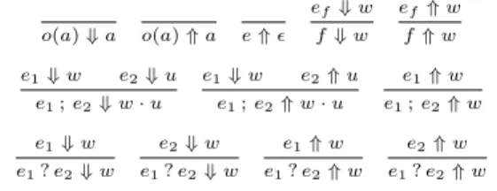
A. Trace Semantics

Let Σ

^≤ω

be the set of all finite and infinite sequences generated from the set Σ of primitive events. We call an element w in Σ

^≤ω

a trace. Given traces w and u, we define the concatenation w · u as:

wu if w ∈ Σ

^∗

and w if w ∈ Σ

^ω

where Σ

^∗

and Σ

^ω

are respectively sets of all finite and infinite sequences over Σ. So, Σ

^≤ω

= Σ

^∗

∪Σ

^ω

and Σ

^∗

= Σ

⁺

∪{}. As usual, we may write wu instead of w·u. We are concerned with finite prefixes of the trace generated by a given expression. We call them observed traces. Notice that all observed traces are in Σ

^∗

. Let e

f

be the definition (a well-formed expression) of f . The observed trace semantics is given in Figure 2. We write

o(a)⇓a o(a)⇑a e⇑ ef⇓w

f⇓w

ef ⇑w f⇑w e₁⇓w e₂⇓u

e1;e2⇓w·u

e₁⇓w e₂⇑u e1;e2⇑w·u

e₁⇑w e1;e2⇑w e₁⇓w

e₁?e₂⇓w

e₂⇓w e₁?e₂⇓w

e₁⇑w e₁?e₂⇑w

e₂⇑w e₁?e₂⇑w

Figure 2.

The Observed Trace Semantics

e ⇓ w to mean that the finite trace generated by e is w. In particular,