Journal of Climate
EARLY ONLINE RELEASE
This is a preliminary PDF of the author-produced manuscript that has been peer-reviewed and accepted for publication. Since it is being posted so soon after acceptance, it has not yet been copyedited, formatted, or processed by AMS Publications. This preliminary version of the
manuscript may be downloaded, distributed, and cited, but please be aware that there will be visual differences and possibly some content differences between this version and the final published version.
The DOI for this manuscript is doi: 10.1175/JCLI-D-16-0200.1
The final published version of this manuscript will replace the preliminary version at the above DOI once it is available.
If you would like to cite this EOR in a separate work, please use the following full citation:
Ummenhofer, C., A. Biastoch, and C. Boening, 2016: Multi-decadal Indian Ocean variability linked to the Pacific and implications for pre-conditioning Indian Ocean Dipole events. J. Climate. doi:10.1175/JCLI-D-16-0200.1, in press.
© 2016 American Meteorological Society
AMERICAN
METEOROLOGICAL
SOCIETY
Multi-decadal Indian Ocean variability linked
1
to the Pacific and implications for
2
pre-conditioning Indian Ocean Dipole events
3
Caroline C. Ummenhofer
∗Department of Physical Oceanography, Woods Hole Oceanographic Institution, Woods Hole, MA, USA
4
Arne Biastoch, Claus W. B¨ oning
GEOMAR Helmholtz Centre for Ocean Research Kiel, Germany
5
∗Corresponding author address: Caroline C. Ummenhofer, Department of Physical Oceanography, Woods Hole Oceanographic Institution, Woods Hole, MA, USA; cummenhofer@whoi.edu
source file Click here to download LaTeX File (.tex, .sty, .cls, .bst, .bib)
Ummenhofer.etal_2016_rev2.tex
ABSTRACT
6
The Indian Ocean has sustained robust surface warming in recent decades, but
7
the role of multi-decadal variability remains unclear. Using ocean model hind-
8
casts, characteristics of low-frequency Indian Ocean temperature variations are
9
explored. Simulated upper-ocean temperature changes across the Indian Ocean
10
in the hindcast are consistent with those recorded in observational products and
11
ocean reanalyses. Indian Ocean temperatures exhibit strong warming trends
12
since the 1950s limited to the surface and south of 30◦S, while extensive subsur-
13
face cooling occurs over much of the tropical Indian Ocean. Previous work fo-
14
cused on diagnosing causes of these long-term trends in the Indian Ocean over the
15
second half of the 20th Century. Instead, the temporal evolution of Indian Ocean
16
subsurface heat content is shown here to reveal distinct multi-decadal variations
17
associated with the Pacific Decadal Oscillation and the long-term trends are thus
18
interpreted to result from aliasing of the low-frequency variability. Transmission
19
of the multi-decadal signal occurs via an oceanic pathway through the Indone-
20
sian Throughflow and is manifest across the Indian Ocean centered along 12◦S
21
as westward propagating Rossby waves modulating thermocline and subsurface
22
heat content variations. Resulting low-frequency changes in the eastern Indian
23
Ocean thermocline depth are associated with decadal variations in the frequency
24
of Indian Ocean Dipole (IOD) events, with positive IOD events unusually com-
25
mon in the 1960s and 1990s with a relatively shallow thermocline. In contrast,
26
the deeper thermocline depth in the 1970s and 1980s is associated with frequent
27
negative IOD and rare positive IOD events. Changes in Pacific wind forcing in
28
recent decades and associated rapid increases in Indian Ocean subsurface heat
29
content can thus affect the basin’s leading mode of variability, with implications
30
for regional climate and vulnerable societies in surrounding countries.
31
1. Introduction
32
Changes over the past two decades in upper-ocean temperatures in the Indian Ocean
33
have recently received increasing attention (e.g., Vialard 2015). The Indian Ocean 100–
34
300m depth layer has warmed significantly since 2003 (Nieves et al. 2015). Rapid increases
35
are also seen in the top 700m Indian Ocean heat content since the early 2000s (Lee et al.
36
2015), concurrent with an increased heat transport from the Pacific to the Indian Ocean
37
through the Indonesian Throughflow (ITF), following enhanced Pacific Ocean heat uptake.
38
The latter had been implicated in recent slower global surface temperature increases during
39
a sustained cooling period in the equatorial Pacific associated with a negative phase of the
40
Interdecadal Pacific Oscillation (IPO; e.g., Kosaka and Xie 2013; England et al. 2014). Lee
41
et al. (2015) proposed that the rapid increase in Indian Ocean heat content accounted for
42
more than 70% of the global upper 700m heat content gain during the past decade. Given
43
these rapid changes underway in the Indian Ocean and their implications for global climate, it
44
is of interest to better understand low-frequency behavior in upper-ocean thermal properties
45
in the Indian Ocean over past decades. Here, we assess multi-decadal variations in the Indo-
46
Pacific using high-resolution ocean general circulation model (OGCM) hindcasts to provide
47
a longer context for the recent upper-ocean thermal changes in the Indian Ocean. This is
48
important for understanding whether recent Indian Ocean temperature changes reflect long-
49
term trends (e.g., Alory et al. 2007; Cai et al. 2008) or whether they are a manifestation of
50
(multi-)decadal variability. We also evaluate whether Indo-Pacific background changes on
51
such timescales have implications for interannual Indian Ocean variability.
52
Tropical Indian Ocean sea surface temperature (SST) generally warmed faster during
53
the period 1950–2010 than the tropical Atlantic or Pacific (Han et al. 2014a). In particular
54
western Indian Ocean SST have warmed by 1.2◦C over the period 1901–2012, making the
55
western Indian Ocean the largest contributor to the overall global SST trend (Roxy et al.
56
2014). Schott et al. (2009) considered the Indian Ocean SST warming trend to exhibit
57
“puzzling subbasin-scale features which are difficult to explain with surface heating alone.”
58
Considerable uncertainty exists about the sign of the net heat flux into or out of the Indian
59
Ocean in some parts (Yu et al. 2007): best estimates do not indicate an increase in heat flux
60
into the Indian Ocean, but a likely negative heat flux trend unable to explain surface warming
61
(Schott et al. 2009). In contrast, Alory and Meyers (2009) attributed the surface warming
62
to a decrease in upwelling-related ocean cooling over the thermocline dome region, arising
63
from reduced wind-driven Ekman pumping; a negative heat flux results, driven by a negative
64
feedback through evaporation, compounded by strengthening trade winds due to equatorial
65
warming. As summarized by Han et al. (2014a), near-surface Indian Ocean warming has
66
been associated with anthropogenic greenhouse gases (e.g., Gregory et al. 2009; Gleckler
67
et al. 2012, and references therein) through changes in downward longwave radiation and
68
weakened winds suppressing turbulent heat loss from the ocean (Du and Xie 2008). However,
69
the weakened winds and changes in heat loss are inconsistent with observed wind and heat
70
flux trends (Yu and Weller 2007). The heat flux dilemma led Schott et al. (2009) to conclude
71
that ocean dynamics must be playing a role in determining upper-ocean temperature trends
72
in the Indian Ocean.
73
It was also noted that top 700m Indian Ocean heat content did not increase during the
74
second half of the 20th Century (Schott et al. 2009), a signal distinct from other (tropical)
75
ocean basins (e.g., Balmaseda et al. 2013). Investigating temperature trends above 1000m in
76
the Indian Ocean Thermal Archive and climate models for the period 1960–1999, Alory et al.
77
(2007) found pronounced warming in the subtropical Indian Ocean 40◦–50◦S extending down
78
to 800m and attributed this to a southward shift in the subtropical gyre due to strengthening
79
westerlies. A concurrent Indian Ocean subsurface cooling in the tropics was associated with
80
more frequent negative Indian Ocean Dipole (IOD) events and a strengthened subtropical
81
cell (Trenary and Han 2008), and a shoaling thermocline (Han et al. 2006; Cai et al. 2008)
82
in response to changing Pacific wind forcing (Alory et al. 2007; Schwarzkopf and B¨oning
83
2011). The leading mode of upper-ocean Indo-Pacific temperatures in the Simple Ocean
84
Data Assimilation product was also found to exhibit a long-term trend of surface warming
85
and subsurface cooling at thermocline depth, which Vargas-Hernandez et al. (2014, 2015)
86
linked to Pacific modes of climate variability, such as the IPO, North Pacific gyre, and
87
El Ni˜no Modoki. Using sensitivity experiments with an OGCM, Schwarzkopf and B¨oning
88
(2011) found the Indian Ocean subsurface cooling trend to be reproduced in simulations
89
with observed wind forcing in the Pacific only, while wind stress outside the Pacific was
90
kept at climatology. This highlights the role of remote Pacific wind forcing for upper-ocean
91
temperature changes in the Indian Ocean.
92
It is well known that signals from remote Pacific wind forcing can be transmitted through
93
the ITF region and result in thermocline depth and sea level variations along Western Aus-
94
tralia, linked through coastal wave dynamics (Clarke and Liu 1994; Meyers 1996; Wijffels and
95
Meyers 2004; Ummenhofer et al. 2013; Sprintall et al. 2014). On interannual timescales, the
96
El Ni˜no-Southern Oscillation (ENSO) is the dominant driver, with the remote signal initi-
97
ated by zonal wind anomalies in the central Pacific and transmitted by westward-propagating
98
Rossby waves in the Pacific, becoming coastally trapped waves at the intersection of the equa-
99
tor and New Guinea (Wijffels and Meyers 2004). Along the Australian coastline, they travel
100
poleward and radiate Rossby waves into the southern Indian Ocean (e.g., Cai et al. 2005).
101
Shi et al. (2007) found the energy transmission from the Pacific to the Indian Ocean during
102
ENSO events to be stronger after 1980 than before. Trenary and Han (2013) used OGCM
103
experiments to assess the relative role of local Indian Ocean versus remote Pacific forcing on
104
subsurface south Indian Ocean decadal variability. Focusing on decadal thermocline varia-
105
tions in the 5◦–17◦S latitude range, they found these to be dominated by Ekman pumping
106
through windstress curl variations over the southern Indian Ocean. However from the 1990s
107
onwards, these thermocline variations were primarily driven by changes in the Pacific trade
108
winds (Trenary and Han 2013).
109
Equatorial zonal easterlies in the Pacific have been strengthening since the late 1990s
110
associated with a negative IPO phase (England et al. 2014). Trends in Pacific equatorial
111
wind stress can directly impact Indian Ocean upper-ocean thermal properties, transmit-
112
ted through the ITF. The ITF transport has been strengthening at 1 Sv/decade during
113
1984–2013 according to a 30-yr expendable bathythermograph record between Fremantle in
114
Western Australia and Sunda Strait (Indonesia; Liu et al. 2015). Using an 18-year ITF
115
proxy transport time-series, developed from in situ measurements and altimetry, Sprintall
116
and Revelard (2014) found significant increases in volume transport in the upper layer of
117
Lombok Strait and over the full depth in Timor Passage since the early 1990s. This was also
118
reflected in OGCM hindcast simulations in higher transport of the ITF and Leeuwin Current
119
along the west coast of Australia post-1993 (Feng et al. 2011). More frequent Ningaloo Ni˜no
120
events (Feng et al. 2013), characterized by anomalously warm ocean conditions off Western
121
Australia, were seen since the 1990s when positive heat content anomalies and cyclonic wind
122
anomalies off Western Australia favored increased southward heat transport by the Leeuwin
123
Current, and were often pre-conditioned by SST in the far western Pacific (Marshall et al.
124
2015). In addition to the well-known equatorial pathway transmitted through coastal wave
125
dynamics through the ITF region, a pathway from the subtropical North Pacific was also
126
proposed (Cai et al. 2005). However, it is unknown how the strength of this Pacific-Indian
127
Ocean transmission varies on longer multi-decadal timescales (Shi et al. 2007).
128
Changes in the eastern Indian Ocean background state on decadal timescales in turn have
129
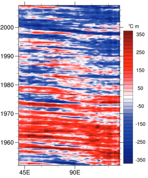
the potential to impact the leading mode of interannual variability in the Indian Ocean, the
130
IOD (Saji et al. 1999; Webster et al. 1999). Annamalai et al. (2005) proposed that an altered
131
background state of the eastern Indian Ocean thermocline on decadal timescales could pre-
132
condition decades for strong positive IOD events. Investigating the rare occurrence of three
133
consecutive positive IOD events observed in 2006–2008 (Cai et al. 2009c), Cai et al. (2009d)
134
proposed an anthropogenic contribution, as positive IOD events became more frequent over
135
the period 1950–1999 in climate models. This was considered consistent with a weaker Walker
136
circulation over the Pacific and changing land-sea temperature gradients over the Indian
137
Ocean. However, subsurface ocean conditions were found to be key for the development
138
(and prediction) of the rare IOD events in 2006–2008, with the triggering mechanism for
139
such an event lying in the ocean (Cai et al. 2009c). It remains unclear, though, what role
140
multi-decadal variability plays in low-frequency changes in the occurrence of both positive
141
and negative IOD events. On interannual timescales, Indian Ocean SST linked to the IOD
142
have been found to impact regional climate in Indian Ocean rim countries (e.g., Webster
143
et al. 1999; Abram et al. 2003; Ashok et al. 2003, 2004; Cai et al. 2009a,b; Ummenhofer
144
et al. 2009b,c, 2011; D’Arrigo et al. 2011; Garcia-Garcia et al. 2011). Given the IOD’s
145
importance for regional climate in vulnerable societies in Indian Ocean rim countries, it
146
is important to better understand how slowly evolving upper-ocean thermal properties on
147
multi-decadal timescales could pre-condition IOD events.
148
Here, we use hindcasts with a high-resolution OGCM to characterize multi-decadal vari-
149
ations in the upper-ocean thermal structure of the Indian Ocean. Focus is on two specific
150
objectives: (1) to examine the nature and origin of the low-frequency evolution of subsurface
151
temperatures in the Indian Ocean; (2) to investigate the implications of these low-frequency
152
thermal variations in the Indian Ocean for the IOD.
153
2. Data and Methods
154
a. Data sets
155
A series of monthly global gridded observational and reanalysis products were used to
156
assess decadal variability in thermal properties across the Indian and Pacific Oceans. At 1◦
157
horizontal resolution this includes EN4.0.2. by the UK Met Office (1900–present; Good et al.
158
2013), which uses quality controlled subsurface ocean temperature and salinity profiles and
159
objective analyses to also provide uncertainty estimates. The Ocean Reanalysis System 4
160
(ORAS4; 1958–present; Balmaseda et al. 2013) by the European Centre for Medium Range
161
Weather Forecasting (ECMWF) uses a sophisticated data assimilation methodology that
162
includes a model bias correction to estimate the state of the global ocean via the operational
163
system Ocean-S4. The ocean model is forced by atmospheric daily surface fluxes, relaxed
164
to SST and bias corrected (CDG 2014). The Pacific Decadal Oscillation (PDO) time-series
165
used consists of standardized values derived as the leading principal component of monthly
166
SST anomalies in the North Pacific north of 20◦N following Mantua et al. (1997).
167
b. Ocean model simulations
168
A series of global OGCM simulations was analyzed, building on an ocean/sea ice model.
169
ORCA025 is an established eddy-active configuration at 0.25◦ nominal resolution (Barnier
170
et al. 2006) based on the Nucleus for European Modelling of the Ocean (NEMO version
171
3.1.1; Madec 2008). The effective resolution in the Indian Ocean varies between 21 and
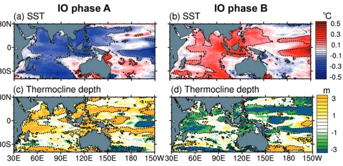
172
28 km in the Indian Ocean, resolving the mesoscale equatorwards of ∼30◦N/S (Hallberg
173
2013). In the vertical, the model is discretized with 46 z-levels, starting with 10 levels in
174
the upper 100m and increasing to a thickness of 250m at depth. The bottom grid cells
175
are allowed to be partially filled, which in combination with an advanced advection scheme
176
results in an improved global circulation (Barnier et al. 2006). Mixed layer dynamics and the
177
vertical mixing are parameterized according to a turbulent kinetic energy scheme (Blanke
178
and Delecluse 1993), lateral mixing is rotated and performed on isopycnals.
179
The model starts from rest, with temperatures and salinities being initialized from a
180
compilation of different observational data sets, in the Indian Ocean taken from the Levi-
181
tus et al. (1998) climatology. For atmospheric forcing conditions of wind and thermohaline
182
fluxes, we used the Large and Yeager (2009) data set, which is originally based on the
183
National Centers for Environmental Prediction (NCEP)/National Center for Atmospheric
184
Research (NCAR) reanalysis products and corrected and globally balanced using various
185
observational data sets. The forcing fields are provided at 6-hourly (wind, air temperature
186
and humidity), daily (short- and longwave radiation) and monthly (precipitation, runoff)
187
resolution and applied through bulk formulae according to the Coordinated Ocean-ice Ref-
188
erence Experiment, CORE-II protocol (Griffies et al. 2009). The ocean model is spun up
189
over the period 1978–2007; based on this, the hindcast integration was performed over the
190
full period 1948–2007.
191
The simulations used very weak sea surface salinity restoring at a 1-yr timescale (Behrens
192
et al. 2013). This aspect is of particular importance in the context of this study for an almost
193
free evolution of surface quantities. To identify and correct for spurious model drift, the sim-
194
ulation was repeated with global climatological (the “normal year” CORE product) forcing.
195
The linear trends for the period 1952-2007 in the climatological simulation were subtracted
196
from all interannually forced simulations. The trends in the climatological simulation are
197
typically almost an order of magnitude smaller than the long-term trends in the simulations
198
using interannual forcing.
199
3. Temperature trends in ocean reanalysis and hindcast
200
To assess the representation of Indian Ocean subsurface thermal properties in the ocean
201
model, the linear trend in our hindcast is compared with the ORAS4 product for 1960–
202
1999, an analysis period used in previous studies (e.g., Alory et al. 2007; Alory and Meyers
203
2009; Schwarzkopf and B¨oning 2011). The linear trend of the Indian Ocean zonal mean
204
temperature for the top 700m reveals surface warming on the order of 0.02◦C/yr in the top
205
50m across the Indian Ocean, extending deeper to 100–200m south of 20◦S in both ORAS4
206
and the ORCA hindcast (Fig. 1a,b). Also apparent is a strong subsurface cooling signal
207
at 60–400m depth for 8◦–15◦S; this subsurface cooling is stronger in the ORCA hindcast
208
(0.03–0.06◦C/yr) than in ORAS4 (Fig. 1a,b). This prominent tropical subsurface cooling
209
was found in previous observational and model-based studies (e.g., Han et al. 2006; Alory
210
et al. 2007; Cai et al. 2008; Trenary and Han 2008; Schwarzkopf and B¨oning 2011) and
211
proposed to be partially linked to changing (Pacific) wind forcing.
212
As can be seen here exemplarily for the 190m depth level for both ORAS4 and ORCA
213
(Fig. 1c,d), the subsurface cooling trend centers at 12◦S and extends across the entire tropical
214
Indian Ocean. The spatial pattern of the tropical subsurface cooling trend compares well
215
between ORAS4 and ORCA, both across the Indian Ocean and for the extensive cooling
216
seen in the Pacific 20◦N–10◦S. Also apparent is the warming in the southern Indian Ocean,
217
centered at 30◦S (Fig. 1c,d) that has previously been associated with a southward shift of
218
the subtropical gyre (Alory et al. 2007).
219
Zonal cross-sections of the temperature trend centered along the equator and along 10◦S
220
further highlight the associated depth-structure (Fig. 1e–h): strong warming in excess of
221
0.025◦C/yr is restricted to a thin surface layer extending to 100m (less than 50m) depth
222
along the equator (at 10◦S); the surface warming trend in the eastern equatorial Indian
223
Ocean is stronger in ORAS4 than in our ORCA hindcast (Fig. 1e,f). The strong subsurface
224
cooling in excess of 0.1◦C/yr is especially prominent in the 10◦S cross-section, extending
225
over the 60–400m depth-range and across the entire width of the Indian Ocean (Fig. 1g,h).
226
For the equatorial cross-section, the subsurface cooling in the ORCA hindcast is limited to
227
the 100–320m depth range in the western Indian Ocean and somewhat narrower in the East,
228
while it extends below 400m in the West (300m in the East) in ORAS4 (Fig. 1e,f).
229
Overall, the spatial patterns of multi-decadal Indian Ocean (subsurface) temperature
230
trends in our ORCA simulations compare well with the trends in the ORAS4 product. Cau-
231
tion needs to be used when analyzing trends in the observational-based EN4 product in
232
data-sparse regions, as the objectively analyzed EN4 gridded temperature in the absence
233
of any observations is relaxed to the 1971–2000 climatology (Good et al. 2013). With this
234
caveat in mind and especially relevant in the data-sparse Indian Ocean, subsurface temper-
235
ature trends in the ORCA simulations across the Indian Ocean are also in broad agreement
236
with the subsurface temperature trends, albeit weak and patchy, in the observational-based
237
EN4 product (figure not shown). This gives us confidence that the OGCM hindcast ex-
238
hibits sufficient skill in representing low-frequency upper-ocean thermal variations across
239
the Indo-Pacific for the present work. Previous studies have also used ORCA simulations
240
for understanding links between Pacific forcing and Indian Ocean variability on interannual
241
(Ummenhofer et al. 2013) and decadal (Schwarzkopf and B¨oning 2011) timescales; they
242
provide further details on the model’s representation of Indo-Pacific upper-ocean variability.
243
In light of these striking upper-ocean temperature trends in the Indian Ocean, it is of
244
interest to explore the temporal evolution of subsurface heat content in the Indo-Pacific.
245
In particular, we are interested in better understanding how these well-described long-term
246
trends relate to the evolution of the upper-ocean thermal structure of the Indian Ocean
247
on multi-decadal timescales. Ocean model hindcasts represent a tool well-suited to this
248
endeavor due to the fact that they are based on a dynamically consistent framework, allow
249
for an almost free evolution of ocean surface quantities, and do not employ infilling of missing
250
data based on climatology for a subset of decades. The latter makes observational or ocean
251
reanalysis products that relax to climatology in the absence of observations (Good et al.
252
2013) or use data assimilation (Stammer et al. 2016) problematic for trend analysis on
253
multi-decadal timescales and beyond. However, comparing Indian Ocean mean temperature
254
trends in the 1990s and 2000s based on various observational-based products and ocean
255
reanalyses, Nieves et al. (2015) found ORAS4 temperature trends in the top 400m to be
256
consistent with those obtained from the World Ocean Atlas (WOA; Levitus et al. 2012) and
257
the Ishii et al. (2005) dataset, while several other reanalysis products exhibited diverging
258
trends. Agreement between ORAS4 and the WOA and Ishii dataset below 500m was reduced
259
(Nieves et al. 2015). Consequently, and due to the apparent disagreement in the temperature
260
trend below 400m in parts of the Indian Ocean between ORAS4 and the ORCA simulations
261
(cf. Fig. 1e,f), we focus our following analyses on the 100–320m depth range.
262
4. Temporal evolution of Indian Ocean heat content
263
and links to the Pacific
264
Subsurface heat content anomalies for 8-yr intervals were calculated as the integrated
265
temperature for the depth-range 100–320m relative to the analysis period 1952–2007 (Fig. 2).
266
The period 1952–1959 was characterized by warm heat content anomalies in the western and
267
central Pacific (15◦S–30◦N; Fig. 2a). The Indonesian-Australian basin extending towards the
268
central Indian Ocean exhibited warm heat content anomalies in the 1950s, but over the 1960s
269
warm heat content anomalies extended westward across much of the Indian Ocean 0–20◦S
270
(Fig. 2a,b). Over the period 1968–1975, warm anomalies weakened in the western Pacific
271
and across the Indian Ocean (Fig. 2c). From 1976 onwards, cool heat content anomalies
272
appeared in the western Pacific, intensifying over the 1980s (Fig. 2d,e). By the early 1990s,
273
cool heat content anomalies expanded northwestward from the eastern Indian Ocean (10◦–
274
30◦S, 80◦–120◦E), reaching the western Indian Ocean in the 2000s (Fig. 2e–g).
275
The westward expansion of anomalous high subsurface heat content in the 1960s and
276
1970s across the Indian Ocean is also apparent in a longitude-time Hovm¨oller plot (Fig. 3).
277
After the 1990s, cooler anomalies in heat content similarly expanded westward across the
278
Indian Ocean (Fig. 3). The spatial pattern of the westward expansion/spreading of the heat
279
content anomaly in the Indian Ocean is reminiscent to the one described by Ummenhofer
280
et al. (2013) on interannual timescales. This was associated with Rossby waves radiating
281
into the southern Indian Ocean, transmitting the ENSO signal to the Indian Ocean, as
282
detected in variations in the depth of the 20◦C-isotherm for example (Cai et al. 2005).
283
On interannual timescales, Xie et al. (2002) found southwest Indian Ocean thermocline
284
variance to be highly correlated with eastern Pacific SST conditions at a lag of 3 months,
285
transmitted through downwelling Rossby waves propagating westward at a phase speed of
286
35◦/yr in the 8◦–12◦S latitude range in the Indian Ocean. Westward propagating baroclinic
287
Rossby waves play an important role in the southern Indian Ocean circulation in the 8◦–15◦S
288
latitude range (e.g., Masumoto and Meyers 1998; Jury and Huang 2004; Baquero-Banal and
289
Latif 2005; Chowdary et al. 2009; Schott et al. 2009). Furthermore, the Indian Ocean’s
290
South Equatorial Current distributes ITF waters across the Indian Ocean, with the bulk
291
of the transport occurring within the thermocline layer (Gordon et al. 1997, and references
292
therein). Observed ITF transport based on expendable bathythermograph (XBT) lines, in
293
situ measurements, and altimetry has increased since the 1980s (Liu et al. 2015) and early
294
1990s (Sprintall and Revelard 2014). While enhanced ITF transport is consistent with recent
295
subsurface warming trends in the Indian Ocean since the late 1990s (Lee et al. 2015; Nieves
296
et al. 2015), these ITF trends cannot account for the long-term subsurface cooling trend
297
centered near 10◦S seen for the 1960s to late 1990s. This is despite the fact that ORCA
298
hindcast simulations also detected higher transport of the ITF and Leeuwin Current along
299
Western Australia post-1993 (Feng et al. 2011).
300
Instead, the response of subsurface heat content anomalies in the Indian Ocean to remote
301
Pacific variations on the (multi-)decadal timescales shown here (Fig. 2) is reminiscent of a
302
thermocline response to Rossby wave propagation, as seen on interannual timescales (Um-
303
menhofer et al. 2013). As such, the Indian Ocean subsurface heat content change appears
304
to be a low-frequency adjustment of the thermocline in response to Pacific forcing. It is
305
reminiscent of the well-known adjustment of the western Pacific thermocline depth (Collins
306
et al. 2010; Williams and Grottoli 2010) to equatorial wind stress forcing in the Pacific on
307
decadal timescales (Schwarzkopf and B¨oning 2011). In a similar vein, using an OGCM hind-
308
cast and multi-century climate model simulations, Shi et al. (2007) proposed a multi-decadal
309
variation in the strength of the transmission of the ENSO-associated Rossby wave signal to
310
the Indian Ocean, but found it hard to detect the transmission signal during weak-ENSO
311
periods.
312
To better evaluate the low-frequency evolution of these Indian Ocean subsurface tem-
313
perature variations, Fig. 4a shows the time-series of zonal mean Indian Ocean subsurface
314
(100–320m) temperature for the 5◦–15◦S latitude band. The time-series is characterized by
315
a warm phase extending from the mid-1950s to the mid-1970s (’IO phase A’), followed by
316
a transition period in the late 1970s, and a cool phase from the 1980s onwards (’IO phase
317
B’). The change in the Indian Ocean zonal mean subsurface temperature is on the order of
318
+0.6–+0.8◦ in the high phase to -0.6◦C in the cool phase (Fig. 4a), a considerable temper-
319
ature change in light of the areal extent. This is also reflected in a substantial change in
320
Indian Ocean heat content: during IO phase A, high heat content anomalies dominated for
321
much of the tropical Indian Ocean north of 15◦S, coincident with extensive high anomalies
322
across the Pacific (15◦S–20◦N; Fig. 4c). In contrast, IO phase B exhibited cool heat content
323
anomalies in a latitudinal band extending from the eastern Indian Ocean along 5◦–15◦S to
324
the west and across the tropical/subtropical Pacific (Fig. 4e).
325
Given the extensive Pacific Ocean heat content signals seen in the analyses so far (Figs. 2
326
and 4c,e), it is of interest to relate Indian Ocean heat content to low-frequency Pacific vari-
327
ability, namely the PDO. The PDO time-series indicates its prominent cool and warm phases
328
in the 1960s/1970s and the 1980s/1990s, respectively (Fig. 4b). Indo-Pacific heat content
329
anomalies during PDO phase A were very similar to those during IO phase A (Fig. 4c,d),
330
consistent with the large overlap in the periods. In contrast, PDO phase B (1979–1998)
331
exhibited extensive cool heat content anomalies across the Pacific, but only in a small area
332
in the eastern Indian Ocean off the northwest shelf of Australia (Fig. 4f). Spreading of cool
333
heat content anomalies across the Indian Ocean, as seen during IO phase B (1982–2004), was
334
only starting in PDO phase B (Fig. 4e,f). Over the full analysis period 1952–2007, the Indian
335
Ocean subsurface temperature is significantly correlated at a 5–6 yr lag with the PDO index
336
(Pearson correlation coefficient of 0.45; P>0.001) and Western Pacific subsurface tempera-
337
ture for the depth range 100–320m in the 0–12◦N, 135–150◦E region (correlation coefficient
338
of 0.59; P>0.001).
339
As summarized in a review by Newman et al. (2016), North Pacific variability associated
340
with the PDO impacts tropical Pacific variability through variations in the subtropical winds.
341
These in turn modulate the strength of the overturning circulation in the subtropical cells
342
(STCs) in the Pacific, affecting the southward advection of relatively cold extratropical
343
waters, which – through equatorial upwelling – drive air-see feedbacks and thus decadal
344
variability in the tropics. Using observations of the 25.0 kg m−3 potential density surface as
345
a measure of the upper pycnocline, McPhaden and Zhang (2002) showed a slowdown in the
346
STC between the early 1970s and late 1990s, with a transit time of 5–10 years to transmit
347
a signal from the North Pacific to the equator. Depth differences of 25–30m in the western
348
equatorial Pacific upper pycnocline between these two time periods in McPhaden and Zhang
349
(2002), which they tentatively linked to the PDO, exhibit spatial patterns reminiscent of
350
the western Pacific heat content anomalies shown here (Fig. 2). Several other previous
351
studies also related subsurface temperatures/sea surface height/sea level variations in the
352
western Pacific that can be affected by the PDO to (south)eastern Indian Ocean on decadal
353
timescales (e.g., Lee and McPhaden 2008; Schwarzkopf and B¨oning 2011; Nidheesh et al.
354
2013; Vargas-Hernandez et al. 2014), with the relationship strengthening in recent decades
355
(Trenary and Han 2013; Han et al. 2014b; Feng et al. 2015).
356
5. Links between Indian Ocean subsurface temperature
357
variations and IOD events
358
It is important to ascertain how the different Indian Ocean background state in subsur-
359
face heat content relates to upper-ocean properties with relevance to surface expressions.
360
Composite anomalies of SST and thermocline depth during the two different phases, i.e., IO
361
phase A and B identified in Fig. 4, are shown in Fig. 5. The thermocline depth here is taken
362
as the depth corresponding to the base of the mixed layer, which is water with differences
363
in potential density of less than 0.01 kg/m−3. IO phase A (1956–1974) was characterized by
364
anomalously cool SST in excess of -0.5◦C over much of the tropical and subtropical Indian
365
Ocean, with the exception of the far southeastern Indian Ocean along the Western Australian
366
coast and the northwest shelf of Australia (Fig. 5a). At the same time, the thermocline was
367
anomalously deep, especially over the northwest shelf of Australia and in the western Indian
368
Ocean, with anomalies in excess of +3m (Fig. 5c). In contrast, IO phase B (1982–2004)
369
exhibited anomalously warm SST in excess of +0.5◦C in the central tropical and subtropical
370
Indian Ocean and a shallower thermocline depth in the western Indian Ocean and the ITF
371
region (Fig. 5c,d).
372
It has been proposed that the background state of the eastern Indian Ocean thermocline
373
depth can modulate the frequency of occurrence of IOD events on decadal timescales (Anna-
374
malai et al. 2005). The time-series of eastern Indian Ocean (90◦–110◦E, 0–10◦S) thermocline
375
depth reflects interannual variations in excess of ±6m, superimposed on low-frequency vari-
376
ations in the background state of ±2m for a decade or more (blue/red shaded periods in
377
Fig. 6a). The numbers of positive IOD (pIOD) / negative IOD (nIOD) events also exhibit
378
low-frequency variations.
379
To determine whether the frequency of pIOD and nIOD events during periods with a
380
deep or shallow eastern Indian Ocean thermocline were unusual, a boot-strapping technique
381
was used to generate an expected distribution based on random events using all years. The
382
box-and-whisker plots in Fig. 6b summarize these expected distributions for pIOD and nIOD,
383
respectively. Given the uneven number of pIOD and nIOD events, the expected distributions
384
for the two phases can differ. The same applies to the number of years with a deep/shallow
385
thermocline background state. From the boot-strapping method, each actual event also has
386
an error bar associated with it. Where the error bar of the actual event does not overlap
387
with the associated box-and-whisker of the expected distribution, the number of events is
388
significantly different from a sample based on all years at the 98% level.
389
During periods with a deep thermocline background state in the 1970s and 1980s, pIOD
390
events were unusually rare with only 3 (±0.5) events, while 6 (±0.5) nIOD events occurred
391
(Fig. 6b). In contrast, when the eastern Indian Ocean thermocline depth was in a shallow
392
state, such as in the 1960s and 1990s, pIOD events were significantly more common with 6
393
(±0.5) events. Given that the eastern Indian Ocean in its climatological state is characterized
394
by relatively warm SST and a deep thermocline compared to the Pacific and Atlantic (Jansen
395
et al. 2009), a shallower thermocline favored the development of positive Bjerknes-type
396
feedback and allowed for more frequent pIOD events; the number of nIOD events on the other
397
hand was not affected (Fig. 6b). A deepening of the thermocline reinforces the climatological
398
background state, further hampering the development of a positive feedback in thermocline-
399
SST coupling over the eastern Indian Ocean; this was reflected in a lower number of pIOD
400
events, while nIOD events were more common. Decadal variations in Indian Ocean SST
401
associated with the IOD have previously been linked to the PDO and IPO (Annamalai
402
et al. 2005; Han et al. 2014b; Dong et al. 2016; Krishnamurthy and Krishnamurthy 2016).
403
Using partial coupling experiments with the Community Climate System Model version 4,
404
Krishnamurthy and Krishnamurthy (2016) proposed a link from the North Pacific to the
405
Indian Ocean excited by northerly wind variations in the western North Pacific.
406
6. Conclusions
407
The Indian Ocean has sustained robust surface warming in the second half of the 20th
408
Century, accompanied by strong tropical subsurface cooling in excess of 0.1◦C/yr especially
409
prominent near 10◦S, extending over the 60–400m depth-range and across the entire width of
410
the Indian Ocean. These spatial patterns of Indian Ocean (subsurface) temperature trends
411
were well-reproduced in the OGCM simulations in this study, when compared to trends in
412
observational/reanalysis products.
413
Previous work focused on diagnosing the thermal structure and cause of these long-term
414
trends in Indian Ocean temperatures in the top 500m over the second half of the 20th Cen-
415
tury. Here, we instead interpret these trends to result from aliasing of the considerable
416
multi-decadal variations that exist in upper-ocean heat content in the Indian Ocean and
417
can be linked to broader Indo-Pacific low-frequency variability: the 1950s were character-
418
ized by warm heat content anomalies in the western and central Pacific. In the Indian
419
Ocean, the Indonesian-Australian basin extending towards the central Indian Ocean ex-
420
hibited warm heat content anomalies in the 1950s, but over the 1960s warm heat content
421
anomalies extended westward across much of the Indian Ocean 0–20◦S. From 1976 onwards,
422
cool anomalies appeared in the western Pacific, intensifying over the 1980s. By the early
423
1990s, cool anomalies expanded northwestward from the eastern Indian Ocean, reaching the
424
western Indian Ocean in the 2000s. To better evaluate the low-frequency evolution of these
425
Indian Ocean subsurface temperature variations, we determined a warm phase extending
426
from the mid-1950s to the mid-1970s, followed by a transition period in the late 1970s, and
427
a cool phase from the 1980s onwards. These related to low-frequency Pacific variability,
428
namely the PDO: lead-lag relationships between Indian Ocean subsurface temperatures re-
429
vealed a multi-year lag with the PDO and western Pacific subsurface temperatures at 5–6
430
years, potentially mediated through an adjustment of the STC and equatorial upwelling in
431
the Pacific (McPhaden and Zhang 2002).
432
Variations in subsurface heat content coincide with changes in the thermocline depth over
433
the eastern Indian Ocean. Changes in the background state of the eastern Indian Ocean ther-
434
mocline have been proposed to modulate the frequency of occurrence of strong positive IOD
435
events on decadal timescales (Annamalai et al. 2005). The eastern Indian Ocean thermocline
436
depth in our hindcast simulations here indeed reflected considerable low-frequency variations.
437
The numbers of pIOD/nIOD events also exhibited low-frequency variations: pIOD events
438
occurred significantly more (less) frequently during periods with a shallow (deep) thermo-
439
cline, while nIOD events were more common when the thermocline was deep. Our results
440
demonstrate that changes in the background state of the subsurface Indian Ocean affect the
441
dominant mode of Indian Ocean interannual variability (IOD). Our results also have impli-
442
cations for decadal predictions. In fact, the Indian Ocean stands out as the region globally
443
where SST state-of-the-art decadal climate predictions for the 2–9 year range perform best
444
(Guemas et al. 2013). They attribute this to the Indian Ocean being the region with the
445
lowest ratio of internally generated over externally forced variability, which is consistent with
446
our findings here.
447
Acknowledgments.
448
Use of the following data sets is gratefully acknowledged: ORAS4 from ECMWF, EN4 from the UK
449
Met Office. The integration of the OGCM experiments was performed at the North-German Supercom-
450
puting Alliance (HLRN) and the Computing Centre at Kiel University. We thank Gary Meyers for helpful
451
discussions and three anonymous reviewers for their comments. This research was supported by a Research
452
Fellowship by the Alexander von Humboldt Foundation, as well as the Ocean Climate Change Institute and
453
theInvestment in Science Fund at WHOI.
454
455
REFERENCES
456
Abram, N. J., M. K. Gagan, M. T. McCulloch, J. Chappell, and W. S. Hantoro, 2003: Coral
457
reef death during the 1997 Indian Ocean Dipole linked to Indonesian wildfires. Science,
458
301, 952–955.
459
Alory, G. and G. Meyers, 2009: Warming of the upper equatorial Indian Ocean and changes
460
in the heat budget (1960-99). Journal of Climate, 22, 93–113.
461
Alory, G., S. Wijffels, and G. Meyers, 2007: Observed temperature trends in the In-
462
dian Ocean over 1960–1999 and associated mechanisms. Geophysical Research Letters,
463
34 (L02606), doi:10.1029/2006GL028 044.
464
Annamalai, H., J. Potemra, R. Murtugudde, and J. P. McCreary, 2005: Effect of precondi-
465
tioning on the extreme climate events in the tropical Indian Ocean. Journal of Climate,
466
18, 3450–3469.
467
Ashok, K., Z. Guan, N. H. Saji, and T. Yamagata, 2004: Individual and combined influences
468
of the ENSO and Indian Ocean Dipole on the Indian summer monsoon.Journal of Climate,
469
17, 3141–3155.
470
Ashok, K., Z. Guan, and T. Yamagata, 2003: Influence of the Indian Ocean
471
Dipole on the Australian winter rainfall. Geophysical Research Letters, 30 (15),
472
doi:10.1029/2003GL017 926.
473
Balmaseda, M. A., K. Mogensen, and A. T. Weaver, 2013: Evaluation of the ECMWF
474
ocean reanalysis system ORAS4. Quarterly Journal of the Royal Meteorological Society,
475
139, 1132–1161.
476
Baquero-Banal, A. and M. Latif, 2005: Wind-driven oceanic Rossby waves in the tropical
477
South Indian Ocean with and without an active ENSO.Journal of Physical Oceanography,
478
35, 729–746.
479
Barnier, B., et al., 2006: Impact of partial steps and momentum advection schemes in a
480
global ocean circulation model at eddy permitting resolution. Ocean Dynamics, 56, 543–
481
567.
482
Behrens, E., A. Biastoch, and C. W. B¨oning, 2013: Spurious AMOC trends in global ocean
483
sea-ice models related to subarctic freshwater forcing.Ocean Modelling, 69, 39–49.
484
Blanke, B. and P. Delecluse, 1993: Variability of the tropical Atlantic Ocean simulated by
485
a general circulation model with two different mixed-layer physics. Journal of Physical
486
Oceanography, 23, 1363–1388.
487
Cai, W., T. Cowan, and M. Raupach, 2009a: Positive Indian Ocean Dipole events pre-
488
condition southeast Australia bushfires. Geophysical Research Letters, 36 (L19710),
489
doi:10.1029/2009GL039 902.
490
Cai, W., T. Cowan, and A. Sullivan, 2009b: Recent unprecedented skewness towards positive
491
Indian Ocean Dipole occurrences and their impact on Australian rainfall. Geophysical
492
Research Letters, 36 (L11705), doi:10.1029/2009GL037 604.
493
Cai, W., G. Meyers, and G. Shi, 2005: Transmission of ENSO signal to the Indian Ocean.
494
Geophysical Research Letters, 32 (L05616), doi:10.1029/2004GL021 736.
495
Cai, W., A. Pan, D. Roemmich, T. Cowan, and X. Guo, 2009c: Argo profiles a rare occur-
496
rence of three consecutive positive Indian Ocean Dipole events, 2006–2008. Geophysical
497
Research Letters, 36 (L08701), doi:10.1029/2008GL037 038.
498
Cai, W., A. Sullivan, and T. Cowan, 2008: Shoaling of the off-equatorial south Indian
499
Ocean thermocline: Is it driven by anthropogenic forcing? Geophysical Research Letters,
500
35 (L12711), doi:10.1029/2008GL034 174.
501
Cai, W., A. Sullivan, and T. Cowan, 2009d: Climate change contributes to more frequent con-
502
secutive positive Indian Ocean Dipole events.Geophysical Research Letters,36 (L23704),
503
doi:10.1029/2009GL040 163.
504
CDG, 2014: Climate Data Guide: ORAS4: ECMWF ocean reanalysis and derived
505
ocean heat content. Tech. rep., Retrieved from https://climatedataguide.ucar.edu/climate-
506
data/oras4-ecmwf-ocean-reanalysis-and-derived-ocean-heat-content; accessed May 2015.
507
Chowdary, J. S., C. Gnanaseelan, and S. P. Xie, 2009: Westward propagation of barrier layer
508
formation in the 2006–07 Rossby wave event over the tropical southwest Indian Ocean.
509
Geophysical Research Letters, 36 (L04607), doi:10.1029/2008GL036 642.
510
Clarke, A. J. and X. Liu, 1994: Interannual sea level in the northern and eastern Indian
511
Ocean.Journal of Physical Oceanography, 24, 1224–1235.
512
Collins, M., et al., 2010: The impact of global warming on the tropical Pacific and El Ni˜no.
513
Nature Geoscience, 3, 391–397.
514
D’Arrigo, R., N. Abram, C. Ummenhofer, J. Palmer, and M. Mudelsee, 2011: Reconstructed
515
streamflow for Citarum River, Java, Indonesia: linkages to tropical climate dynamics.
516
Climate Dynamics, 36, 451–462.
517
Dong, L., T. Zhou, A. Dai, F. Song, B. Wu, and X. Chen, 2016: The footprint of the Inter-
518
decadal Pacific Oscillation in Indian Ocean sea surface temperatures. Scientific Reports,
519
6 (21251), doi:10.1038/srep21 251.
520
Du, Y. and S.-P. Xie, 2008: Role of atmospheric adjustments in the tropical Indian
521
Ocean warming during the 20th century in climate models.Geophysical Research Letters,
522
35 (L08712), doi:10.1029/2008GL033 631.
523
England, M. H., et al., 2014: Recent intensification of wind-driven circulation in the Pacific
524
and the ongoing warming hiatus. Nature Climate Change, 4, 222–227.
525
Feng, M., C. B¨oning, A. Biastoch, E. Behrens, E. Weller, and Y. Masumoto, 2011: The
526
reversal of the multi-decadal trends of the equatorial Pacific easterly winds, and the
527
Indonesian Throughflow and Leeuwin Current transports. Geophysical Research Letters,
528
38 (L11604), doi:10.1029/2011GL047 291.
529
Feng, M., H. H. Hendon, S.-P. Xie, A. G. Marshall, A. Schiller, Y. Kosaka, N. Caputi,
530
and A. Pearce, 2015: Decadal increase in Ningaloo Ni˜no since the late 1990s.Geophysical
531
Research Letters, 42, 104–112.
532
Feng, M., M. J. McPhaden, S.-P. Xie, and J. Hafner, 2013: La Ni˜na forces unprecedented
533
Leeuwin Current warming in 2011. Scientific Reports,3, doi:10.1038/srep01 277.
534
Garcia-Garcia, D., C. C. Ummenhofer, and V. Zlotnicki, 2011: Australian water mass vari-
535
ations from GRACE data linked to Indo-Pacific climate variability. Remote Sensing of
536
Environment, 115, 2175–2183.
537
Gleckler, P. J., et al., 2012: Human-induced global ocean warming on multidecadal
538
timescales. Nature Climate Change, 2, 524–529.
539
Good, S. A., M. J. Martin, and N. A. Rayner, 2013: EN4: quality controlled ocean tem-
540
perature and salinity profiles and monthly objective analyses with uncertainty estimates.
541
Journal of Geophysical Research: Oceans,118, 6704–6716.
542
Gordon, A. L., S. Ma, D. B. Olson, P. Hacker, A. Ffield, L. D. Talley, D. Wilson, and
543
M. Baringer, 1997: Advection and diffusion of Indonesian Throughflow water within the
544
Indian Ocean South Equatorial Current. Geophysical Research Letters, 24 (21), 2573–
545
2576.
546
Gregory, J. M., H. T. Banks, P. A. Stott, J. A. Lowe, and M. D. Palmer, 2009: Simulated
547
and observed decadal variability in ocean heat content. Geophysical Research Letters,
548
31 (L15312), doi:10.1029/2004GL020 258.
549
Griffies, S. M., et al., 2009: Coordinated Ocean-ice Reference Experiments (COREs).Ocean
550
Modelling, 26, 1–46.
551
Guemas, V., S. Corti, J. Garcia-Serrano, F. J. Doblas-Reyes, M. Balmaseda, and L. Mag-
552
nusson, 2013: The Indian Ocean: The region of highest skill worldwide in decadal climate
553
prediction. Journal of Climate, 26, 726–739.
554
Hallberg, R., 2013: Using a resolution function to regulate parameterizations of oceanic
555
mesoscale eddy effects. Ocean Modeling, 72, 92–103.
556
Han, W., G. A. Meehl, and A. Hu, 2006: Interpretation of tropical thermocline cooling
557
in the Indian and Pacific oceans during recent decades. Geophysical Research Letters,
558
33 (L23615), doi:10.1029/2006GL027 982.
559
Han, W., H. Vialard, M. J. McPhaden, T. Lee, Y. Masumoto, M. Feng, and W. P. M.
560
de Ruijter, 2014a: Indian Ocean decadal variability: A review. Bulletin of the American
561
Meteorological Society,97, 1679–1703.
562
Han, W., et al., 2014b: Intensification of decadal and multi-decadal sea level variability in
563
the western tropical Pacific during recent decades.Climate Dynamics, 43, 1357–1379.
564
Ishii, M., A. Shouji, S. Sugimoto, and T. Matsumoto, 2005: Objective analyses of sea-surface
565
temperature and marine meteorological variables for the 20th century using ICOADS and
566
the Kobe Collection.International Journal of Climatology,25, 865–879.
567
Jansen, M. F., D. Dommenget, and N. Keenlyside, 2009: Tropical atmosphere-ocean inter-
568
actions in a conceptual framework.Journal of Climate, 22, 550–567.
569
Jury, M. R. and B. Huang, 2004: The Rossby wave as a key mechanism of Indian Ocean
570
climate variability. Deep Sea Research I, 51, 2123–2136.
571
Kosaka, Y. and S.-P. Xie, 2013: Recent global-warming hiatus tied to equatorial Pacific
572
surface cooling. Nature,501, 403–407.
573
Krishnamurthy, L. and V. Krishnamurthy, 2016: Decadal and interannual variability of the
574
Indian Ocean SST.Climate Dynamics, 46, 57–70.
575
Large, W. and S. Yeager, 2009: The global climatology of an interannually varying air-sea
576
flux data set. Climate Dynamics, 33, 341–364.
577
Lee, S.-K., W. Park, M. O. Baringer, A. L. Gordon, B. Huber, and Y. Liu, 2015: Pacific
578
origin of the abrupt increase in Indian Ocean heat content during the warming hiatus.
579
Nature Geoscience, 8, 445–450.
580
Lee, T. and M. J. McPhaden, 2008: Decadal phase change in large-scale sea level and winds
581
in the Indo-Pacific region at the end of the 20th century. Geophysical Research Letters,
582
35 (L01605), doi:10.1029/2007GL032 419.
583
Levitus, S., et al., 1998: World ocean database 1998, volume 1: Introduction. Tech. rep.,
584
NOAA Atlas NESDIS 18, U.S. Government Printing Office, Washington, D.C.
585
Levitus, S., et al., 2012: World ocean heat content and thermosteric sea level change (0–2000
586
m), 1950–2010. Geophysical Research Letters, 39 (L10603), doi:10.1029/2012GL051 106.
587
Liu, Q.-Y., M. Feng, D. Wang, and S. Wijffels, 2015: Interannual variability of the Indonesian
588
Throughflow transport: a revisit based on 30-year expendable bathythermograph data.
589
Journal of Geophysical Research - Oceans, 120, 8270–8282.
590
Madec, G., 2008: NEMO ocean engine, version 3.1. Tech. rep., Note Pˆole Model. Inst.
591
Pierre-Simon Laplace, Paris, 27, ISSN,12881619, 27 pp.
592
Mantua, N. J., S. R. Hare, Y. Zhang, J. M. Wallace, and R. C. Francis, 1997: A Pacific inter-
593
decadal climate oscillation with impacts on salmon production. Bulletin of the American
594
Meteorological Society,78, 1069–1079.
595
Marshall, A. G., H. H. Hendon, M. Feng, and A. Schiller, 2015: Initiation and amplification
596
of the Ningaloo Ni˜no. Climate Dynamics, 45, 2367–2385.
597
Masumoto, Y. and G. Meyers, 1998: Forced Rossby waves in the southern tropical Indian
598
Ocean.Journal of Geophysical Research, 103 (C12), 27 589–27 602.
599
McPhaden, M. J. and D. Zhang, 2002: Slowdown of the meridional overturning circulation
600
in the upper Pacific Ocean. Nature, 415, 603–608.
601
Meyers, G., 1996: Variation of Indonesian Throughflow and the El-Ni˜no-Southern Oscilla-
602
tion. Journal of Geophysical Research, 101, 12 255–12 263.
603
Newman, M., et al., 2016: The Pacific Decadal Oscillation revisited.Journal of Climate,29,
604
4399–4427.
605
Nidheesh, A. G., M. Lengaigne, J. Vialard, A. S. Unnikrishnan, and H. Dayan, 2013: Decadal
606
and long-term sea level variability in the tropical Indo-Pacific Ocean.Climate Dynamics,
607
41, 381–402.
608
Nieves, V., J. K. Willis, and W. C. Patzert, 2015: Recent hiatus caused by decadal shift in
609
Indo-Pacific heating.Science, 349, 532–535.
610
Roxy, M. K., K. Ritika, P. Terray, and S. Masson, 2014: The curious case of Indian Ocean
611
warming.Journal of Climate, 27, 8501–8509.
612