Testing for stationarity of functional time series in the frequency domain

SFB 823

Testing for stationarity of

functional time series in the frequency domain

Discussion Paper Alexander Aue, Anne van Delft

Nr. 19/2019

Testing for stationarity of functional time series in the frequency domain

Alexander Aue^† Anne van Delft^‡ May 1, 2019

Abstract

Interest in functional time series has spiked in the recent past with papers covering both methodology and applications being published at a much increased pace. This article contributes to the research in this area by proposing a new stationarity test for functional time series based on frequency domain methods.

The proposed test statistics is based on joint dimension reduction via functional principal components analysis across the spectral density operators at all Fourier frequencies, explicitly allowing for frequency- dependent levels of truncation to adapt to the dynamics of the underlying functional time series. The properties of the test are derived both under the null hypothesis of stationary functional time series and under the smooth alternative of locally stationary functional time series. The methodology is theoretically justified through asymptotic results. Evidence from simulation studies and an application to annual tem- perature curves suggests that the test works well in finite samples.

Keywords: Frequency domain methods, Functional data analysis, Locally stationary processes, Spectral analysis

MSC 2010:Primary: 62G99, 62H99, Secondary: 62M10, 62M15, 91B84

1 Introduction

The aim of this paper is to provide a new stationarity test for functional time series based on frequency domain methods. Particular attention is given to taking into account alternatives allowing for smooth variation as a source of non-stationarity, even though non-smooth alternatives are covered within the simulation study.

Functional data analysis has seen an upsurge in research contributions for at least one decade. This is reflected in the growing number of monographs in the area. Readers interested in the current state of statistical inference procedures may consult Bosq (2000), Ferraty & Vieu (2010), Horv´ath & Kokoszka (2012), Hsing & Eubank (2015) and Ramsay & Silverman (2005).

∗AA was partially supported by NSF grants DMS 1305858 and DMS 1407530. AvD was partially supported by Maastricht University, the contract “Projet d’Actions de Recherche Concert´ees” No. 12/17-045 of the “Communaut´e franc¸aise de Belgique” and by the Collaborative Research Center “Statistical modeling of nonlinear dynamic processes” (SFB 823, Project A1, C1, A7) of the German Research Foundation (DFG).

†Department of Statistics, University of California, Davis, CA 95616, USA, email:aaue@ucdavis.edu

‡Ruhr-Universit¨at Bochum, Fakult¨at f¨ur Mathematik, 44780 Bochum, Germany, email:Anne.vanDelft@rub.de

arXiv:1701.01741v3 [stat.ME] 29 Apr 2019

Papers on functional time series have come into the focus more recently and constitute now an active area of research. H¨ormann & Kokoszka (2010) introduced a general weak dependence concept for stationary func- tional time series, while van Delft & Eichler (2018a) provided a framework for locally stationary functional time series. Antoniadis & Sapatinas (2003), Aue et al. (2015) and Besse et al. (2000) constructed prediction methodology that may find application across many areas of science, economics and finance. With the ex- ception of van Delft & Eichler (2018a), the above contributions are concerned with procedures in the time domain. Complementing methodology in the frequency domain has been developed in parallel. One should mention Panaretos & Tavakoli (2013), who provided results concerning the Fourier analysis of time series in function spaces, and H¨ormann et al. (2015), who addressed the problem of dimension reduction for functional time series using dynamic principal components.

The methodology proposed in this paper provides a new frequency domain inference procedure for func- tional time series. More precisely, tests for second-order stationarity are developed. In the univariate case, such tests have a long history, going back at least to the seminal paper Priestley & Subba Rao (1969), who based their method on the evaluation of evolutionary spectra of a given time series. Other contributions build- ing on this work include von Sachs & Neumann (2000), who used local periodograms and wavelet analysis, and Paparoditis (2009), whose test is based on comparing a local estimate of the spectral density to a global estimate. Dette et al. (2011) and Preuß et al. (2013) developed methods to derive both a measure of and a test for stationarity in locally stationary time series, the latter authors basing their method on empirical process theory. In all papers, interest is in smoothly varying alternatives. The same tests, however, also tend to have power against non-smooth alternatives such as structural breaks or change-points. A recent review discussing methodology for structural breaks in time series is Aue & Horv´ath (2013), while Aue et al. (2018) is a recent contribution to structural breaks in functional time series.

The proposed test for second-order stationarity of functional time series seeks to exploit that the Discrete Fourier Transform (DFT) of a functional time series evaluated at distinct Fourier frequencies are asymptot- ically uncorrelated if and only if the series is second-order stationary. The proposed method is therefore related to the initial work of Dwivedi & Subba Rao (2011), who put forth similar tests in a univariate frame- work. Their method has since been generalized to multivariate time series in Jentsch & Subba Rao (2015) as well as to spatial and spatio-temporal data by Bandyopadhyay & Subba Rao (2017) and Bandyopadhyay et al.

(2017), respectively. A different version of functional stationarity tests, based on time domain methodology involving cumulative sum statistics (Aue & Horv´ath, 2013), was given in Horv´ath et al. (2014).

The intrinsic variation of a functional time series is always larger than any sample size, and standard results known from univariate and multivariate time series analysis do not directly apply. From a practical perspective this brings to the fore the question of how to compress this infinite-dimensional variation to finite dimension in a meaningful way, as there is a complex interplay between dynamics occurring across frequencies and the function space. This means that dimension reduction has to be done jointly across estimated spectral density operators at all Fourier frequencies, yet separately as the exact level of dimension reduction has to be decided

per frequency. The proposed test statistics collect these different sets of projections, obtained via functional principal components analysis, into a quadratic form encapsulating the second-order dynamics. To derive the large-sample behavior of this statistic under both the null hypothesis of a stationary time series and the alterna- tive of a locally stationary functional time series requires new, and perhaps independently interesting, results on distributional convergence of a cross-periodogram operator in function space, where verifying existence of the limit process and tightness are nontrivial tasks. The subsequent proofs of distributional convergence of the test statistics which require taking into account the pecularities of fPCA estimators, are also complex and new.

The main results are derived under the assumption that the curves are observed in their entirety, corresponding to a setting in which functions are sampled on a dense grid rather than a sparse grid. Differences for these two cases have been worked out in Li & Hsing (2010).

The remainder of the paper is organized as follows. Section 2 provides background, gives requisite nota- tions, introduces properties of functional version of the DFT and gives intuition for the test. The exact form of the hypothesis test, model assumptions and the test statistics are introduced in Section 3. The large-sample behavior under the null hypothesis of second-order stationarity and the alternative of local stationarity is es- tablished in Sections 4. Empirical aspects are highlighted in Section 5. The proofs are technical and relegated to the Appendix. Several further auxiliary results are proved in the supplementary document Aue & van Delft (2019), henceforth referred to simply as the Online Supplement.

2 Notation and setup

A functional time seriespX_t:tPZqwill be viewed as a sequence of random elements on a probability space pΩ,A, Pq with paths in a separable Hilbert space. Without loss of generality, we shall focus on processes taking values inH_R“L²_Rpr0,1sq, the space of equivalence classes of real-valued, square integrable functions on the unit intervalr0,1s. Because the methodology introduced in this paper is based on a frequency domain approach, we shall make extensive use of the complex Hilbert spaceH “ L²

Cpr0,1sq. We briefly introduce notation and relevant properties of this space and associated operators. The complex conjugate ofz P Cis denoted byzand the imaginary number byi. Forf, gPH, the inner product and the inducedL2-norm onH are respectively given by

xf, gy “ ż₁

0

fpτqgpτqdτ and }f}2 “a

xf, fy. (2.1)

Two elements of H are understood to be equal if their difference has vanishingL₂-norm. More generally, for measurable functionsg: r0,1s^k Ñ C, theL^p-norm shall be denoted by}g}_p and the supremum norm by }g}8“sup_τPr0,1s^k|gpτq|.

Next, some properties of linear operators onHare stated. Denote byS₈pHqthe Banach space of bounded linear operatorsA:H Ñ H equipped with the operator norm~A~₈ “sup_}g}2ď1}Ag}₂. For allf, g PH, the adjoint operator ofA, denoted byA^:, is defined byxAf, gy “ xf, A^:gyand the conjugate operator ofA

is given byAg “ pAgq. An operatorAis called self-adjoint ifxAf, gy “ xf, Agyfor allf, g P Hand non- negative definite ifxAg, gy ě0for allgPH. ForvPH, define the tensor productfbg:HbH ÑHas the bounded linear operatorpfbgqv“ xv, gyf. A compact operatorAadmits asingular value decomposition

A“

8

ÿ

n“1

snpAqψnbφn, (2.2)

where ps_npAq: n P Nq, are the singular values ofA, pφ_n: n P Nq and pψ_n: n P Nq orthonormal bases ofH. The singular values are ordered to form a monotonically decreasing sequence of non-negative num- bers. A compact operator A is said to belong to the Schatten p-class SppHq if and only if the sequence spAq “ ps_npAq: n P Nq of singular values of A belongs to the sequence space `^p, so if and only if

~A~_p “ př₈

n“1s^p_npAqq^1{p ă 8, where ~A~_p is referred to as the Schatten p-norm. Relevant here are S1pHq, the space of trace-class operators, and particularlyS2pHq, the space of Hilbert–Schmidt operators.

The latter is also a Hilbert space with inner product xA, ByS “ ř₈

i“1xAψi, Bψiy where A, B P S2pHq andpψ_n: n P Nqis an ONB of H. The mappingT: HbH Ñ S₂pHq defined by the linear extension of Tpfbgq “fbgis an isometric isomorphism and defines a Hilbert–Schmidt operator with kernel inHˆH given bypf bgqpτ, σq “ fpτqgpσq,τ, σ P r0,1s. As a consequence,A P S2pHqif and only if there exists aPHˆH such that~A~2 “ }a}2. Further useful properties needed in the proofs of the various statements of this paper are relegated to the Appendix and the Online Supplement.

2.1 Dependence structure on the function space Let L²

CpΩq be the Hilbert space with elements satisfiying Er}X}²₂s ă 8 and denote by ErXs the mean function ofX, where the expectation should be viewed in the sense of a Bochner integral. ForX, Y PL²

CpΩq, the covariance operator CX,Y: H bH Ñ H is defined as CX,Y “ ErpX ´ErXsq b pY ´ErYsqs and belongs toS2pHq. A functional time seriesX “ pXt:tPZqis called strictly stationary if, for all finite sets of indicesJ Ă Z, the joint distribution ofpX_{t`j</sub>:j PJqdoes not depend ontP Z. Similarly,X is weakly stationary if its first- and second-order moments exist and are invariant under translation in time. Without loss of generality, it is assumed throughout thatErXts “ 0and that Xt P L<sup>2</sup><sub>R</sub>pΩq for allt P Z. The lag-h covariance operator betweenXtandX<sub>t`h}is denoted by

Ct,h“ErXt`hbXts

which reduces to Ch “ ErX_h bX₀sin case of weak stationarity. Note that this object is a non-negative definite element ofS1pH_Rqforh“0. The covariance operatorChcan be shown to form a Fourier pair with a non-negative Hermitian element ofSppHq. Provided sufficiently fast decay of the second-order structure, the spectral density operatorFωis well-defined and given by the Fourier transform ofCh,

Fω “ 1 2π

ÿ

hPZ

Che^´iωh. (2.3)

A sufficient condition for the existence ofFωinS_ppHqisř

hPZ~Ch~pă 8.

Higher-order dependence among the functional observations is defined through cumulant mixing condi- tions (Brillinger, 1981; Brillinger & Rosenblatt, 1967). For this, the notion of higher-order cumulant tensors is required; see Appendix B for their definition and a discussion of their properties for nonstationary functional time series.

2.2 The functional discrete Fourier transform

The starting point of this paper is the following proposition that characterizes second-order stationary behavior of a functional time series in terms of a spectral representation. Its proof is in Appendix A.

Proposition 2.1. A zero-mean, H-valued stochastic process pX_t: t P Zq whose spectral measure is trace class admits the representation

X_t“ ż_π

´π

e^itωdZ_ω a.s., (2.4)

wherepZω:ω P p´π, πsqis a right-continuous functional orthogonal-increment process, if and only if it is weakly stationary.

If the process is not weakly stationary, then a representation in the frequency domain is not necessar- ily well-defined and certainly not with respect to complex exponential basis functions. However, a time- dependent functional Cram´er representation exists if the characteristics of the process are captured by a Bochner-measurable mapping that is an evolutionary operator-valued mapping in time direction (van Delft

& Eichler, 2018a). Assume that the functions X₁, . . . , X_T have been observed. If the process is weakly stationary, thefunctional Discrete Fourier Transform(fDFT) evaluated at frequencyω, given by

D_ω^pTq“ 1

?2πT

T

ÿ

t“1

Xte^´iωt, (2.5)

can be seen as an estimate of the increment processZ_ω and exists almost surely as an element ofH. The functional time series itself can then be represented through the inverse fDFT as

Xt“ c2π

T

T

ÿ

j“1

D^pT_ωj^qe^iωjt. (2.6)

Under regularity conditions, a set of fDFTs evaluated at distinct frequencies yield asymptotically independent Gaussian random elements inH and, for fixedω, one hasVarpD^pTω ^qq Ñ Fω (Panaretos & Tavakoli, 2013).

The fDFT sequence of a Hilbertian-valued stationary process is in particular asymptotically uncorrelated at the canonical frequenciesωj “2πj{T. Consequently, provided the series is weakly stationary, forj ‰j¹ or j ‰T ´j¹, we have~CovpDω^pTj^q, Dω^pT_j1^qq~2 “Op1{Tq. In other words, the lag-hcovariance operator of the fDFT converges in norm and hence weak operator topology to the zero operator asT Ñ 8. Similar to the above, the reverse argument (uncorrelatedness of the functional DFT sequence implies weak stationarity) can

be shown by means of the inverse fDFT. Using expression (2.5), the covariance operatorCt,hofX_t`handX_t can be written in terms of the fDFT sequence as

Ct,h “ 2π T

T

ÿ

j,j¹“1

ErD^pT_ωj^qbD_ω^pTq

j1se^iωjh “ 2π T

T

ÿ

j“1

ErD_ω^pT_j^qbD_ω^pT_j^qse^iωjh “Ch,

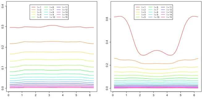
where the equality holds in anL²-sense. This demonstrates that the autocovariance kernel of a second-order stationary functional time series is obtained and, hence, that an uncorrelated fDFT sequence implies second- order stationarity up to lagT´1. The fDFT thus captures exactly the defining property of a weakly stationary process and provides a natural starting point for a test of stationarity. It is, however, a nontrivial task to construct a test statistic that optimally extracts the information contained in the infinite-dimensional process to finite dimensions. Not only can the dependence structure and the resulting dynamics of a functional time series be of a complicated nature (see Figure 5.1 and the example given in Section S8 of the Online Supplement), but the process will vary along both frequency and functional directions. To construct a powerful test it is therefore crucial to understand how the fDFT’s behave when weak stationarity is violated. In accordance with aforementioned time series literature, the theoretical behavior of the fDFT sequence under smooth alternatives is studied. These properties will then be exploited to verify large-sample results for a testing framework for functional stationarity.

3 The functional stationarity testing framework

This section gives precise formulations of the hypotheses of interest, states the main assumptions of the paper and introduces the test statistics. Throughout, interest is in testing the null hypothesis

H0:pXt:tPZqis a weakly stationary functional time series versus the alternative

H_A:pX_t:tPZqis a locally stationary functional time series, where locally stationary functional time series are defined as follows.

Definition 3.1. A stochastic processpXt:tPZqtaking values inH_Ris said to be locally stationary if (1) X_t“X_t^pTqfort“1, . . . , T andT PN; and

(2) for any rescaled timeuP r0,1s, there is a strictly stationary processpX_t^puq:tPZqsuch that

›

›X_t^pTq´X_t^puq›

›2ď

´ˇ ˇ ˇ

t T ´u

ˇ ˇ ˇ`_T¹

¯

P_t,T^puq a.s.,

whereP_t,T^puqis a positive, real-valued triangular array of random variables such that, for someρ ą0, Er|P_t,T^puq|^ρs ă 8for alltandT, uniformly inuP r0,1s.

Note that, underH_A, the process constitutes a triangular array of functions. Inference methods are then based on in-fill asymptotics as popularized in Dahlhaus (1997) for univariate time series. The process is then considered to be observed on a finer grid asT increases such that more observations are available at a local level. A rigorous statistical framework for locally stationary functional time series was recently provided in van Delft & Eichler (2018a). Note that weakly stationary processes are included in Definition 3.1, which then reduces to standard asymptotics.

Based on the observations in Section 2.2, a test for weak stationarity can be set up exploiting the uncor- relatedness of the elements in the sequencepDω^pTj^q:j “1, . . . , Tq. This could be done considering the lag-h sample covariance operatorT^´1ř_T

j“1Dω^pTj^qbDω^pT<sub>j`h</sub><sup>q</sup> which should be centered at the zero operator inS<sub>2</sub>for allh “ 1, . . . , T ´1. Here, two statistics based on the coefficients in the Karhunen–Lo`eve decomposition of the fDFTs are considered. For j “ 1, . . . , T, letpφ^ω_l^j: l P Nq be the orthonormal basis of eigenfunc- tions of Fωj and observe that for this choice of basis VarpxD_ωj, φ^ω_l^jyq “ xFωjpφ^ω_l^jq, φ^ω_l^jy “ λ^ω_l^j, where pλ^ω_l^j:l PNq PR`are the eigenvalues ofFωj. Then, for anyj, j¹,pφ^ω_l^j bφ^ω_l1^j1:l, l¹ PNqis an orthonormal basis ofL²_Cpr0,1s²qand, by definition of the Hilbert–Schmidt inner product on the algebraic tensor product spaceHbH,

1 T

T

ÿ

j“1

D^pT_ωj^qbD_ω^pT_j`h^q “ 1 T

T

ÿ

j“1 8

ÿ

l“1 8

ÿ

l¹“1

@D_ω^pT_j^qbD_ω^pT<sub>j`h</sub><sup>q</sup> , φ<sup>ω</sup><sub>l</sub><sup>j</sup> bφ<sup>ω</sup><sub>l</sub>1<sup>j`h</sup>

D

Sφ^ω_l^j bφ^ω_l1^j`h (3.1)

« 1 T

T

ÿ

j“1 L

ÿ

l“1 L¹

ÿ

l¹“1

xD^pT_ωj^q, φ^ω_l^jyxD^pTωj`h<sup>q</sup> , φ<sup>ω</sup><sub>l</sub>1<sup>j`h</sup>yφ^ω_l^jbφ^ω_l1^j`h

for sufficiently largeLandL¹. The foregoing motivates to set up tests based on the score products

γ_j,h^pTqpl, l¹q “ xD_ω^pT_j^q, φ^ω_l^jyxDω^pTj`h<sup>q</sup> , φ<sup>ω</sup><sub>l</sub>1<sup>j`h</sup>y (3.2) or on the standardized score products

ρ^pT_j,h^qpl, l¹q “

γ_j,h^pTqpl, l¹q b

λ^ω_l^jλ^ω_l1^j`h

. (3.3)

In practice, the unknown spectral density operatorsFωj andFωj`h are to be replaced with consistent estima- torsFˆω<sup>pT</sup>j<sup>q</sup>andFˆ<sup>pT</sup>ωj`h^q , which will then yield respective sample eigenvaluesλˆ^ω_l^j and eigenfunctionsφˆ^ω_l^j. The estimated quantities corresponding to (3.2) and (3.3) will be denoted byˆγ_j,h^pTqpl, l¹qandρˆ^pT_j,h^qpl, l¹q, respectively.

As an estimator ofFω, take

Fˆω^pTq“ 2π T

T

ÿ

j“1

K_bpω´ωjq`

D^pT_ωj^qbD^pT_ωj^q˘

, (3.4)

whereK_bp¨qis a kernel with bandwidthbsatisfying the following conditions.

Assumption 3.1. (a) LetK:r´¹₂,¹₂s ÑR`be symmetric withş

Kpxqdx“1andş

Kpxq²dxă 8.

(b) Letb“b_T be a bandwidth such thatT^´1{2 !b_T !T^´1{4.

(c) LetKbpxq “b^´1Kpp2πbq^´1xqand and extend the kernel periodically such thatKbpxq “Kbpx˘2πq in order to include estimates for frequencies around˘π.

To set up the test statistics, it now appears reasonable to extract information across a range of directions l “ 1, . . . , L_j andl¹ “ 1, . . . , L<sub>j`h</sub> as well as a selection of lagsh “ 1, . . . ,¯h, where ¯hdenotes an upper limit. The truncation parameters Lj “ Lpωjq and Lj`h “ Lpωj`hq are explicitly allowed to depend on thej-th andpj`hq-th Fourier frequencies in order to accommodate heterogeneity in the Karhunen–Lo`eve decompositions across the spectral domain. Set

βˆ^pT_h,u^q“ 1 T

T

ÿ

j“1 Lj

ÿ

l“1 Lj`h

ÿ

l¹“1

ˆ

γ_j,h^pTqpl, l¹q and βˆ_h,s^pTq“ 1 T

T

ÿ

j“1 Lj

ÿ

l“1 Lj`h

ÿ

l¹“1

ˆ

ρ^pT_j,h^qpl, l¹q, (3.5) where the subscriptsuandsrefer to the un-standardized and standardized forms, respectively. In the follow- ing, the subscriptxwill be used to refer to any of these two versions when no confusion can arise.

Choose next a collection h₁, . . . , h_M of lags each of which is upper bounded by ¯h to pool information across a number of autocovariances and build the vectors

ˆb^pT_M,x^q “`

<βˆ_h^pTq

1,x, . . . ,<βˆ^pT_h ^q

M,x,=βˆ_h^pTq

1,x, . . . ,=βˆ_h^pTq

M,x

˘J

,

where<and=denote real and imaginary part, respectively. Finally, set up the quadratic forms

Qˆ^pT_M,x^q “Tpˆb^pT_M,x^qq^JΣˆ^´1_M,xˆb^pT_M,x^q, (3.6) where ΣˆM,x is an estimator of the asymptotic covariance matrix of the vectors b^pT_M,x^q which are defined by replacingγˆ_j,h^pTqpl, l¹qandρˆ^pT_j,h^qpl, l¹qwithγ_j,h^pTqpl, l¹qandρ^pT_j,h^qpl, l¹qin (3.5) and then using the resultingβ_h,x^pTq in place ofβˆ_h,x^pTq in the definition of ˆb^pT_M,x^q. The foregoing provides the two test statisticsQˆ^pT_M,u^q andQˆ^pT_M,s^q that will be used to test the null of stationarity against the alternative of local stationarity. Note that both quadratic forms depend on the tuning parametersLj,L_j`handM, the selection of which will be evaluated empirically in Section 5.

To facilitate the derivation of large-sample results, the following assumptions are made: for the un- standardized respectively standardized test require

ConditionCu: LetLj „logT andlim_linfωλ^ω_l ą0;

ConditionCs: Letinfωλ^ω_L¯ ą0for someL¯ ěsup_jLj.

In keeping with the above arrangement, the respective conditions will be referred to as C_x if no confusion arises. Condition C_u for the un-standardized test allows to send the truncation levels L_j to infinity in a coordinated manner as long as the divergence is slow (here, logarithmic) compared toT; see Fremdt et al.

(2014). ConditionCs for the standardized test on the other hand requires a finite truncation level, to ensure that the smallest eigenvalues of the compact operatorsFωj are bounded away from zero as these show up in the denominator of (3.3).

4 Large-sample results

4.1 Assumptions

The following gives the main requirements under both stationarity and local stationarity in terms of cumulant tensors of the functional time series (Appendix B) that are needed to establish the asymptotic behavior of the test statistics under both hypotheses. Note that the null hypothesis is nested within the alternative. Because of this basic fact, we start with the general assumptions under local stationarity before specializing to the stationary case.

Assumption I (k,`). AssumepX_t^pTq:t ď T, T P Nq andpX_t^puq:t P Zq are as in Definition 3.1. Suppose sup_tEr}Xt}^minpk,12q₂ s ă 8and that there exists a a positive sequenceκ_{k;t1,...,tk´1} inL²

Rpr0,1s^kq, independent of T such that, for allj“1, . . . , k´1and some`PN,

ÿ

t1,...,tk´1PZ

p1` |tj|<sup>`</sup>q}κ_{k;t1,...,tk´1}}2ă 8. (4.1)

Suppose furthermore that there exist representations

X_t^pTq´X_t^pt{Tq“Y_t^pTq and X_t^puq´X_t^pvq“ pu´vqY_t^pu,vq, (4.2) for some processespY_t^pTq:t ď T, T P NqandpY_t^pu,vq:t P Zq taking values inH_Rwhosek-th order joint cumulants satisfy

(i) }cumpX_t^pTq

1 , . . . , X_t^pTq

k´1, Y_t^pTq

k q}2 ď _T¹}κ_{k;t1´tk,...,tk´1´tk}}2, (ii) }cumpX_t^pu₁^1q, . . . , X_t^pu_k´1^k´1q, Y_t^pu_k ^k,vqq}2ď }κ_{k;t1´tk,...,tk´1´tk}}2, (iii) sup_u}cumpX_t^puq

1 , . . . , X_t^puq

k´1, X_t^puq

k q}2ď }κ_{k;t1´tk,...,tk´1´tk}}2, (iv) sup_u}_Bu<sup>B`</sup>`cumpX_t^puq₁ , . . . , X_t^puq_k´1, X_t^puq_k q}2ď }κ_{k;t1´tk,...,tk´1´tk}}2.

Assumption I provides Lipschitz conditions that are generalizations of those in Lee & Subba Rao (2016), who investigated the properties of quadratic forms of stochastic processes in a finite-dimensional setting. The above conditions enable to express the behavior of the fDFT’s of a k-th order locally stationary process in terms ofk-th order time-varying spectral density tensors (Lemma B.1). This is convenient in order to derive explicit expressions of the distributional properties under the alternative and to understand departures from stationarity. Under H_A, we can uniquely characterize the second-order stucture of the stochastic process pX_t^pTq:tďT, T PNqvia thetime-varying spectral density operator

Fu,ω“ 1 2π

ÿ

hPZ

Cu,he^´iωh, (4.3)

whereCu,h “cumpX_h^puq, X₀^puqqdenotes the local cumulant tensor at fixed timeuof the stationary approximat- ing processpX_t^puq:tPZq. Note that the parameter`and (iii)-(iv) in Assumption I, influence the smoothness of the operator-valued mappingpu, ωq ÞÑ Fu,ω. Under Assumption I(2,2), derivative maps are well-defined

elements ofS₂pHqandω ÞÑ Fu;ω is uniformly continuous inω with respect to~¨~2. We refer to Lemma S2.2 for details. More generally, underk-th order local stationarity, these properties carry over to the local k-th order cumulant spectral density tensor

Fu;ω1,...,ωk´1 “ 1 p2πq^k´1

ÿ

t1,...,tk´1PZ

Cu;t1,...,tk´1e^´i

ř_k´1

j“1ωjtj, (4.4)

whereω₁, . . . , ω_k´1 P p´π, πsandCu;t1,...,tk´1 “ cum`

X_t^puq₁ , . . . , X_t^puq

k´1, X_t^puq₀ ˘

is the corresponding local cumulant kernel tensor of orderkat timeu₀. Observe that, forką 1, (4.4) can be viewed as an element of S2pH^btpk`1q{2u, H^btk{2uq. Underk-th order stationarity the above objects become independent of local timeu, so thatFu;ω1,...,ω_k´1 ”Fω1,...,ω_k´1, and Assumption I specializes to the following.

Assumption I* (k,`). LetpXt: t P Zq be ak-th order stationary functional time series with values inH_R such that (i)Er}X₀}^minpk,12q₂ s ă 8and (ii)ř₈

t1,...,tk´1“´8p1` |t<sub>j</sub>|<sup>`</sup>q}Ct1,...,tk´1}2 ă 8for all1ďj ďk´1.

Because the test statistics require estimators of the eigenelements ofFω, it is of importance to consider the properties of the estimator (3.4) for both null and alternative hypotheses. The next theorem shows that it is a consistent estimator of the integrated (in a Bochner sense) time-varying spectral density operator

G_ω“ ż₁

0

Fu,ωdu,

where the convergence is uniform inω P r´π, πswith respect to~¨~2. This therefore becomes an operator- valued function inωthat acts onHand is independent of rescaled timeu. UnderH₀,G_ωthus reduces toFω.

Theorem 4.1(Consistency and uniform convergence). SupposepX_t^pTq:tďT, T PNqsatisfies Assumption Ip4,2q. Consider the estimatorFˆ^pTω ^q in (3.4) with smoothing kernelK fulfilling Assumption 3.1(a) and (c).

Then,

(a) Er~Fˆω^pTq´G_ω~²₂s “OppbTq^´1`b⁴q, uniformly inωP r´π, πs.

(b) If, in addition, Assumption 3.1(b) holds andKhas bounded derivative onp´1{2,1{2qthen, sup_ωPr´π,πs~Fˆω^pTq´Gω~2

Ñp 0.

The proof of Theorem 4.1 is given in Section C.3 of the Appendix. Since the theorem shows consistency of Fˆω, a self-adjoint element ofS2pHq, it follows from Mas & Menneteau (2003) that the sample eigenelements pλˆ^ω_l,φˆ^ω_l :l P NqofFˆω provide consistent estimators for the eigenelementspλ˜^ω_l,φ˜^ω_l :l PNqofG_ω. IfH₀is satisfied, then the stated consistency holds for the eigenelementspλ^ω_l, φ^ω_l :lPNqofFω.

4.2 Properties under the null of stationarity

The asymptic results under H₀ are collected in this section. The first theorem establishes that the scaled difference betweenβ_h,x^pTqandβˆ^pT_h,x^qis negligible in large samples. Note that the assumptions here and for other

theorems in this section are formulated imposing stationarity on certain moments for the null hypothesis via Assumption I*. To verify the results, typically further assumptions on higher-order cumulants are required.

These are controlled via Assumption I.

Theorem 4.2. Let Assumption 3.1, AssumptionI(12,2) andC_xhold. Then, underH₀, for any fixedh,

?Tˇ

ˇβˆ_h,x^pTq´β_h,x^pTqˇ ˇ“Op

ˆ 1 bT `b²

˙

pT Ñ 8q.

The proof is given in Section D.2.2 of the Appendix. In view of Assumption 3.1, Theorem 4.2 shows that the distributional properties ofβˆ_h,x^pTq are asymptotically the same as those ofβ_h,x^pTq. Note that these rates are necessary for the estimator in (3.4) to be consistent, as is seen from part (a) of Theorem 4.1, which reduces to the stationary case if the process does not depend onu. They hence do not impose an additional constraint underH0.

The next theorem derives that, under the additional assumption of fourth-order stationarity, the asymptotic variance is uncorrelated for all lagshand that there is no correlation between the real and imaginary parts.

FornPN, setrns “ t1, . . . , nu.

Theorem 4.3. Let Assumption 3.1 and C_x hold. Suppose further that AssumptionI*(4,2) is satisfied. Then, forh₁“h₂ “h,

paq TCov

´

<βˆ^pT_h,u^q,<βˆ^pT_h,u^q

¯

“TCov

´

=βˆ^pT_h,u^q,=βˆ^pT_h,u^q

¯

Ñ 1 4π

ż ż ÿ

pl,l¹qPLˆL¹

xFω,´ω´ωh,´ω¹pφ^ω_l1¹

1 bφ^ω_l1^1`ω1h

2 q, φ^ω_l1bφ^ω`ω_l ^h

2 ydωdω¹` 1 2π

ż ÿ

lPL

λ^ω_l1λ^ω`ω_l ^h

2 dω,

pbq TCov

´

<βˆ^pT_h,s^q,<βˆ^pT_h,s^q

¯

“TCov

´

=βˆ^pT_h,s^q,=βˆ^pT_h,s^q

¯

Ñ 1 4π

ż ż ÿ

pl,l¹qPLˆL¹

xFω,´ω´ωh,´ω¹pφ^ω_l1¹

1 bφ^ω_l1^1`ωh1 2 q, φ^ω_l

1 bφ^ω`ω_l ^h

2 y

c λ^ω_l

1λ^ω`ω_l ^h

2 λ^ω_l1¹ 1λ^ω_l1^1`ω1h

2

dωdω¹` 1 2π

ż ÿ

lPL

δ_l1,l2dω,

wherel “ pl₁, l₂q, l¹ “ pl₁¹, l¹₂q, L “ rLpωqs ˆ rLpω`ω<sub>h</sub>qs,L<sup>1</sup> “ rLpω<sup>1</sup>qs ˆ rLpω<sup>1</sup> `ω¹_hqs, andδ_i,j “ 1 if i “ j and 0 otherwise. If h₁ ‰ h₂, TCovp<βˆ^pT_h ^q

1,x,<βˆ_h^pTq

2,xq Ñ 0, TCovp=βˆ_h^pTq

1,x,=βˆ_h^pTq

2,xq Ñ 0 and TCovp<βˆ_h^pTq

1,x,=βˆ_h^pTq

2,xq Ñ0.

The proof of Theorem 4.3 is given in Appendix C.2. Observe that the results in part (b) imply that the standardized test statistics is pivotal if the data is Gaussian. Note also that the results in the theorem use at various instances the fact that thek-th order spectral density operator at frequencyω “ pω1, . . . , ωkq^T PR^k is equal to thek-th order spectral density operator at frequency´ωin the manifoldř_k

j“1ω_j mod 2π.

With the previous results in place, the large-sample behavior of the quadratic form statisticsQˆ^pT_M,x^q defined in (3.6) can be derived. This is done in the following theorem.

Theorem 4.4. Let Assumption 3.1 andC_x hold. Suppose further that AssumptionI(k, 2) is satisfied for all kě3. Then, underH₀,

(a) For any collectionh₁, . . . , h_M bounded by¯h,

?Tbˆ^pT_M,x^q Ñ^D N2Mp0,Σ0,xq pT Ñ 8q,

whereÑ^D denotes convergence in distribution. Under the additional assumption of fourth-order station- arity, N2Mp0,Σ_0,xqis a 2M-dimensional normal distribution with mean 0and diagonal covariance matrixΣ_0,x“diagpσ_0,m,x² :m“1, . . . ,2Mqwhose elements are

σ²_0,m,x “ lim

TÑ8TCov`

<βˆhm,x,<βˆhm,x

˘, m“1, . . . , M,

andσ²_0,M`m,x “σ²_0,m,x. The explicit form of the limit is determined by Theorem 4.3. If fourth-order stationarity is violated, then the limiting normal distribution has a non-diagonal covariance structure.

(b) Using the result in (a), it follows that for the statistic defined in(3.6) Qˆ^pT_M,x^q Ñ^D χ²_2M pT Ñ 8q,

whereχ²_2M is aχ²-distributed random variable with2M degrees of freedom.

The proof of Theorem 4.4 is provided in Appendix D. Part (b) of the theorem can now be used to construct tests with asymptotic levelα. Note that the application of the test requires an estimator ofΣˆ_M,x. This will be discussed in Section 4.4.

To explicitly compute the limiting covariance structure in part (a) of Theorem 4.4 under second-order stationarity but fourth-order nonstationarity, the source of nonstationarity needs to be specified. For example, the results put forward in the next two sections allow for the computation ofΣ_0,xif the process is fourth-order locally stationary. Then, in the covariance structure of the covariance operator of the fDFT’s, the fourth- order cumulant tensor component will, forh1 ‰h2, (quadratically) decay in norm as the distance|h1 ´h2| increases (see Lemma B.1, Corollary B.1 (ii) and equation (C.2)). As a consequence of this term being present in the covariance structure, the real and imaginary part of the projections are no longer uncorrelated but the correlation decays with increasing distance|h₁´h₂|. In this scenario, a small loss of power is to be expected when the test statistic is built under the assumption of a diagonal covariance structure.

4.3 Properties under the alternative

This section contains a generalization of the results in Section 4.2 to locally stationary functional time series.

The following theorem is the counterpart to Theorem 4.2 under the null hypothesis.

Theorem 4.5. Let Assumption 3.1, AssumptionI(12,2) andC_xhold. Then, underH_A,

?TE

”ˇ

ˇβˆ_h,x^pTq´β_h,x^pTq´B^pT_h,x^qˇ ˇ ı

“O ˆ 1

bT `b<sup>2</sup>` 1 b?

T `b²? T

˙

pT Ñ 8q, where

B^pT_h,x^q“ 1 T

T

ÿ

j“1

ÿ

lPL

ζ_l,x@

ErDωjbDω_j`h

‰,Erφˆ^ω_l^jbφˆ^ω_l1^{j`h</sup>s ´φˆ<sup>ω</sup><sub>l</sub><sup>j</sup> bφˆ<sup>ω</sup><sub>l</sub>1<sup>j`h}

D

S

is a stochastic bias term satisfying?

TB^pT_h,x^q “O_Pp1q, andζ_l,u“1andζ_l,s “ p˜λ^ω_l,λ˜^ω`ω_l1 ^hq^´1{2.

The proof of Theorem 4.5 is given in Section D.2.2 of the Appendix. In view of Assumption 3.1, the theorem shows thatβˆ^pT_h,x^qhas the same asymptotic sampling properties asβ_h,x^pTqup to a stochastically bounded bias term (after scaling with?

T). Note that|βˆ_h,x^pTq´Erβ^pT_h,x^qs|Ñ^P 0, where Erβ^pT_h,x^qs Ñ 1

2π ż_2π

0

ż₁

0

ÿ

lPL

ζl,xxFu;ωe^´ı2πuh,φ˜^ω_l bφ˜^ω`ω_l1 ^hySdudω“µh,x (4.5) is an noncentrality parameter (see Appendix C.1) that will have to enter the limit distribution ofQˆ^pT_M,x^q as a consequence of the violation of weak stationarity. We discuss this term in some more detail below.

A precise formulation of the asymptotic properties underHAis given in the next theorem.

Theorem 4.6. Let Assumption 3.1 andC_x hold. Suppose further that AssumptionI(k, 2) is satisfied for all kě2. Then, underHA,

(a) For any collectionh1, . . . , hM bounded by¯h,

?Tˆb^pT_M,x^q Ñ^D N2Mpµ_x,Σ_A,xq pT Ñ 8q,

whereN2Mpµ_x,Σ_A,xqdenotes a2M-dimensional normal distribution with mean vectorµ_xwhose first M components are<µ_hm,xand lastM components are=µ_hm,x, whereµ_hm,xis defined through (4.5), and non-diagonal block covariance matrix

ΣA,x “

¨

˝

Σ^p11q_A,x Σ^p12q_A,x Σ^p21q_A,x Σ^p22q_A,x

˛

‚

whoseM ˆM blocks are determined by the results in Appendix E and Section S6.2 of the Online Supplement.

(b) Using the result in (a), it follows that for the statistic defined in (3.6) Qˆ^pT_M,x^q Ñ^D χ²_µx,2M, pT Ñ 8q, whereχ²_µ

x,2M denotes a generalized noncentralχ²-distributed random variable with noncentrality pa- rameterµx“ }µx}²₂and2M degrees of freedom.

The proof of Theorem 4.6 can be found in Appendix E. Observe that the limiting noncentrality parameter µx of the statisticQˆ^pT_M,x^q measures the aggregation of the functions in (4.5). UnderHA, the operator in (3.1) no longer converges in norm to the zero operator but instead to the operator _2π¹ ş_2π

0

ş₁

0Fu,ωe^´i2πuhdudω. The properties of the latter, which are extracted to finite dimension viaµ_h,x, carry some meaningful information on the behavior of the test under the alternative. Firstly, denote a general term in the limiting expansion of µh,xby

µ_h,xplq “ 1 2π

ż_2π

0

ż₁

0

ζ_l,xxFu;ωe^´i2πuh,φ˜^ω_l bφ˜^ω`ω_l1 ^hySdudω.

For fixed directionsl “ pl, l¹q, this function can be seen to approximate theph,0q-th Fourier coefficients of the functionpu, ωq ÞÑζl,xxFu,ωpφ˜^ω`ω_l1 ^hq,φ˜^ω_ly, i.e., for smallhandT Ñ 8they approximate

ϑ_h,j,xplq “ 1 2π

ż_2π

0

ż₁

0

ζ_l,xxFu,ωφ˜^ω`ω_l1 ^h,φ˜^ω_lye^i2πuh´ijωdudω

with j “ 0. In other words, µ_h,xplq « ϑ_h,0,xplq. If the process is weakly stationary then the integrand of the coefficient does not depend on u and all Fourier coefficients are zero exceptϑ_0,j,xplq. In particular, ϑ0,0,splq “ 1. Following Paparoditis (2009) and Dwivedi & Subba Rao (2011), the mean functions can thus be seen to reveal long-term non-stationary behavior. Unlike testing methods based on segments in the time domain, the proposed method is therefore able to detect smoothly changing behavior in the temporal dependence structure.

Secondly, the operator ş₁

0Fu,ωe^´i2πuhducan be viewed as the h-th Fourier coefficient of the operator- valued functionpuq ÞÑFu,ωfor fixedω(Lemma B.1), which exhibits a quadratic decay in norm as a function ofhsuch that the sum of the norms of these coefficients is finite (Corollary B.1). Since this behavior carries over to the projections, the contribution toµ_xof the functionsµ_h,xin (4.5) for larger values ofhwill become negligible. Intuitively, utilizing large values of M in the statistic Qˆ^pT_M,x^q is hence expected to increase the likelihood of a type II error; see also Section 5.

The results in this and the previous section require an understanding of the estimator Σˆ_M,x used in the definition of the test statisticsQˆ^pT_M,x^q in (3.6). The corresponding results are part of the next subsection.

4.4 Estimating the fourth-order spectrum

The estimation of the matrixΣ_M is a necessary ingredient in the application of the proposed stationarity test.

Generally, the estimation of the sample (co)variance can influence the power of tests, as has been observed in a number of previous works set in similar albeit nonfunctional contexts. Among the contributions more closely related to this paper are Paparoditis (2009) who used the spectral density of the squares, Dwivedi &

Subba Rao (2011), who focused on Gaussianity of the observations, and Jentsch & Subba Rao (2015), who employed a stationary bootstrap procedure. A different idea was put forward by Bandyopadhyay & Subba Rao (2017) and Bandyopadhyay et al. (2017). These authors utilized the notion of orthogonal samples to estimate the variance, falling back on a general estimation strategy developed in Subba Rao (2018).

In order to utilize the results of Theorem 4.4, we require an estimator of the tri-spectral density operator Fω,´ω´ω_h,´ω¹, which can then subsequently be projected onto the (standardized) empirical eigenfunctions and integrated overω, ω¹. As an estimator, consider

Fˆωj1,...,ωj4 “ p2πq³ pb4Tq³

ÿ

k1,k2,k3

K₄

´ωj1 ´ω_k1

b₄ , . . . ,ωj4 ´ω_k4 b₄

¯

Φpω_k1, . . . , ω_k4qI_ω^pT_k^q

1,...,ωk4, (4.6) where

I_ω^pTq

k1,ω_k2,ω_k3,ω_k4 “ T 2πD_ωk

1 bD_ωk

2 bD_ωk

3 bD_ωk

4