AMERICAN METEOROLOGICAL SOCIETY

Journal of Physical Oceanography

EARLY ONLINE RELEASE

This is a preliminary PDF of the author-produced manuscript that has been peer-reviewed and accepted for publication. Since it is being posted so soon after acceptance, it has not yet been copyedited, formatted, or processed by AMS Publications. This preliminary version of the

manuscript may be downloaded, distributed, and cited, but please be aware that there will be visual differences and possibly some content differences between this version and the final published version.

The DOI for this manuscript is doi: 10.1175/JPO-D-14-0171.1

The final published version of this manuscript will replace the preliminary version at the above DOI once it is available.

If you would like to cite this EOR in a separate work, please use the following full citation:

Ascani, F., E. Firing, J. McCreary, P. Brandt, and R. Greatbatch, 2015: The deep equatorial ocean circulation in wind-forced numerical solutions. J. Phys.

Oceanogr. doi:10.1175/JPO-D-14-0171.1, in press.

AMERICAN

METEOROLOGICAL

SOCIETY

The deep equatorial ocean circulation in wind-forced numerical solutions

François Ascani^a,*, Eric Firing^b, Julian P. McCreary^b,c, Peter Brandt^d and Richard J. Greatbatch^d

a Marine Science Department, University of Hawaii at Hilo, 200 W. Kawili St., Hilo, HI 96720 USA

b School of Ocean and Earth Science and Technology, Department of Oceanography, University of Hawaii at Manoa, 1000 Pope Road, Honolulu, HI 96822 USA

cSchool of Ocean and Earth Science and Technology, International Pacific Research Center, University of Hawaii at Manoa, 1680 East-West Road, Honolulu, HI 96822 USA

d GEOMAR Helmholtz-Zentrum für Ozeanforschung Kiel, Kiel, Germany

*Corresponding author address: François Ascani, Marine Science Department, University of Hawaii at Hilo, 200 W. Kawili St., Hilo, HI 96720 USA. E-mail:fascani@hawaii.edu. Phone: 1-808-932- 7575. Fax: 1-808-932-7588.

5

10

15

20

Manuscript (non-LaTeX)

Click here to download Manuscript (non-LaTeX): Ascani_etal_draft.pdf

Abstract

We perform eddy-resolving and high-vertical-resolution numerical simulations of the circulation in an idealized equatorial Atlantic Ocean in order to explore the formation of the deep equatorial circulation (DEC) in this basin. Unlike in previous studies, the deep equatorial intraseasonal variability (DEIV) that is believed to be the source of the DEC is generated internally by instabilities of the upper ocean currents.

Two main simulations are discussed: Solution 1, configured with a rectangular basin and with wind forcing that is zonally and temporally uniform; and Solution 2, with realistic coastlines and with an annual cycle of wind forcing varying zonally. Somewhat surprisingly, Solution 1 produces the more realistic DEC: The large-vertical-scale currents (Equatorial Intermediate Currents or EICs) are found over a large zonal portion of the basin, and the small-vertical-scale equatorial currents (Equatorial Deep Jets or EDJs) form low-frequency, quasi-resonant, baroclinic equatorial basin modes with phase propagating mostly downward, consistent with observations. We demonstrate that both types of currents arise from the rectification of DEIV, consistent with previous theories. We also find that the EDJs contribute to maintaining the EICs, suggesting that the nonlinear energy transfer is more complex than previously thought. In Solution 2, the DEC is unrealistically weak and less spatially coherent than in the first simulation probably because of its weaker DEIV. Using intermediate solutions, we find that the main reason for this weaker DEIV is the use of realistic coastlines in Solution 2. It remains to be determined, what needs to be modified or included to obtain a realistic DEC in the more realistic configuration.

25

30

35

40

1 Introduction

1.1 Overview

The equatorial Atlantic and Pacific Oceans exhibit a complex set of zonal currents at intermediate depths (500−2500 m), typically with an instantaneous amplitude of up to 15−25 cm/s (Fig. 1; Firing 1987; Schottet al. 1995, 2003; Firinget al. 1998; Gouriouet al. 1999, 2001; Bourlèset al. 2002, 2003; Sendet al. 2002; Ollitraultet al. 2006; Eden and Dengler 2008; Ascaniet al. 2010;

Brandtet al. 2011, 2012; Cravatteet al. 2012; Youngs and Johnson 2014). This deep equatorial circulation (DEC; see a list of abbreviations in Tab. 1) is composed of two types of flow: Equatorial Deep Jets (EDJs), which are trapped on the equator and alternate with depth with a vertical wavelength of about 400-600 m; and Equatorial Intermediate Currents (EICs), which have a large vertical scale and alternate with latitude every 1−2° between about 5°S and 5°N¹.

Both sets of currents contribute to the global ocean circulation and the zonal distribution of water masses and biogeochemical quantities. For instance, the eastward jets have been shown to supply dissolved oxygen to the oxygen minimum zone of the deep eastern equatorial Atlantic and Pacific Oceans (Strammaet al. 2005; Eden 2006; Brandtet al. 2008; Strammaet al. 2010;

Czeschelet al. 2011; Brandtet al. 2012). Further, the large-scale biases in the nutrient and oxygen

1 Latitudinally alternating large-vertical-scale zonal jets are also found at more poleward latitudes (see Ollitraultet al. 2006, Cravatteet al. 2012 and Qiuet al. 2013 for a recent account). We do not include them in the present paper but note that the dynamical similarity between these jets and the EICs is still unclear.

45

50

55

60

fields in global, coupled, biogeochemical ocean models have been attributed to inaccuracies of the simulated DEC (Dietze and Loeptien 2013; Getzlaff and Dietze 2013). Finally, Brandtet al. (2011) provide evidence that the upward-propagating energy and interannual variability of the EDJs in the Atlantic Ocean might be indirectly responsible for a portion of the interannual atmospheric variability via their modulation of sea surface temperature (SST).

On the modeling side, a realistic DEC is absent in most ocean general circulation model (OGCM) solutions. At the same time, recent theory and idealized numerical simulations have shown that the DEC may arise from the rectification of the deep equatorial intraseasonal variability (DEIV) (d'Orgevilleet al. 2007; Huaet al. 2008; Ménesguenet al. 2009; Ascaniet al. 2010). The reasons for this inconsistency are not clear. One possible cause is that DEIV, which arises internally from instabilities of the mean circulation in OGCMs, may be poorly reproduced in these models.

1.2 Present research

In this study, we continue the effort to understand DEC dynamics and improve its modeling; for this purpose, we focus on the Atlantic Ocean. Specifically, we seek to reduce the gap between idealized and OGCM simulations by obtaining a series of numerical solutions that generate DEIV internally. We have tested many configurations with varying parameters and degrees of realism. Here, we focus on two: Solution 1, with a rectangular basin and with winds varying only with latitude; and Solution 2, with realistic coastlines and with an annual cycle of zonally and meridionally varying winds based on Atlantic climatology. We also briefly mention the results of two intermediate solutions (Solutions 1.5 65

70

75

80

85

and 1.8) to understand the differences between Solutions 1 and 2. In all solutions, instabilities of the upper-ocean mean equatorial circulation, known as Tropical Instability Waves (TIWs), provide the source for DEIV, and a DEC with some resemblance to Atlantic observations is obtained. Surprisingly, the more realistic DEC is obtained in the more idealized simulation (Solution 1): In particular, the EICs are found over a large zonal portion of the basin and the EDJs form low-frequency, quasi-resonant, baroclinic equatorial basin modes with phase propagating mostly downward, consistent with observations. We then study DEC dynamics by analyzing the zonal kinetic energy budget in Solution 1.

We confirm the results of previous studies, that DEIV is the original source for DEC, but we also discover that the EDJs supply energy to the EICs, suggesting that the nonlinear energy transfer involved in the formation of DEC is more complex than previously assumed.

The paper is organized as follows. Section 2 provides a background for our study, reviewing the temporal and spatial characteristics of the EDJs and EICs in both the Pacific and Atlantic oceans, their simulation in previous idealized and realistic numerical models, and the theories proposed to explain them. Section 3 describes the overall design of our modeling experiments. Section 4 describes the upper-ocean circulation, DEIV, and DEC in Solutions 1 and 2, noting the similarity of the modeled EDJs to low-frequency, baroclinic equatorial basin modes. The results of the two intermediate solutions are also discussed. Section 5 discusses the dynamical processes that link DEIV to the DEC via the analysis of the zonal kinetic energy budget. Section 6 provides a summary and discussion of our results, including implications of the differences between Solutions 1 and 2 for the modeling of DEC in OGCMs.

90

95

100

105

2 Background

In this section, we review the temporal and spatial structure of observed EDJs and EICs, their reproduction in previous numerical models, and the theories proposed to explain them.

2.1 Observations

Multi-year collections of CTD and horizontal velocity data in the Atlantic Ocean provide information on the spatial and temporal characteristics of the EDJs and on their underlying dynamics.

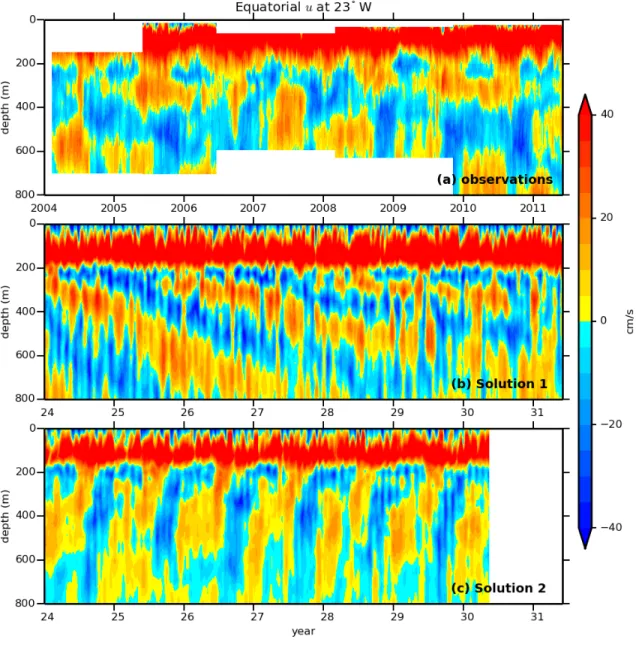
Johnson and Zhang (2003) analyzed the EDJ signature in the vertical strain of density from all available CTD data collected in the Atlantic Ocean, a dataset that spanned about 25 years. They concluded that the Atlantic EDJs have a period of about 5±1 years and exhibit downward phase propagation; consistent with linear equatorial wave theory, the latter property implies upward energy propagation, suggesting that the origin of the EDJs lies in the deep ocean. These properties have been confirmed recently in an 8-year time series of horizontal velocity, obtained from moored measurements (reproduced here in Fig. 2a), from horizontal velocity observations spanning several decades derived from the net displacement of profiling floats (Brandt et al. 2011) and, more recently, from an extensive dataset of Argo and shipboard vertical density profiles (Youngs and Johnson 2015).

The relatively long period and small vertical wavelength of the EDJs are consistent with a dynamical description of the Atlantic EDJs in terms of quasi-resonant, low-frequency, baroclinic 110

115

120

125

equatorial basin modes (Cane and Moore 1981; d'Orgevilleet al. 2007; Bungeet al. 2008; Brandtet al.

2011, 2012). These modes are composed principally of a Kelvin wave and its reflection into a first- meridional-mode long Rossby wave, with the period of the mode (T_n) being a function of the gravity- wave phase speed of the particular baroclinic mode (^cn),

T_n=4L_B

c_n , (1)

where L_B is the width of the basin. The smaller the vertical wavelength, the lower the gravity wave speed and, hence, the longer the period of the mode. For the Atlantic Ocean (L_B ~ 60°), the basin mode associated with vertical modes 14-16 (~600 m vertical wavelength; c_n ~ 20 cm/s) has a period of about 4.2 years, which matches approximately the observed EDJ period. This dynamical interpretation in terms of basin modes is also consistent with the observed meridional structure of the EDJs (Johnson and Zhang 2003; Greatbatch et al. 2012).

In the Pacific Ocean, Firing (1987) observed the EDJs over a 16-month period and did not find any significant vertical migration. Johnsonet al. (2002), however, analyzed the signature of the EDJs in the vertical strain of density in the Pacific Ocean, a dataset that spanned about 22 years. In the eastern Pacific, they found downward phase propagation at a rate suggesting a period of 30±4 years, but noted that inferring periodicity from this dataset is a “dangerous exercise”. In both Firing (1987) and Johnsonet al. (2002), the EDJs corresponded to about vertical mode 32 (c_n ~ 10 cm/s); with the Pacific Ocean being about 140° wide, a basin mode with this vertical scale should have a period of about 20 years, marginally less than the Johnsonet al. (2002)'s estimate. Youngs and Johnson (2015) 130

135

140

145

150

recently analyzed an updated dataset, including 4 years of relatively dense sampling by high-resolution ARGO profiles in the Pacific. They found that the EDJ signal in the Pacific is much weaker in amplitude and broader in bandwidth than that in the Atlantic, making it more difficult to identify a single dominant periodic structure. Nevertheless, they isolated basin-scale zonal and temporal coherence 1.5° on either side of the equator centered at a vertical scale corresponding to mode 22 (^cn ~ 15 cm/s). The phase propagation was downward and to the west, fitting a first-meridional-mode Rossby wave with a period of 12±5 years; for comparison, the period of a basin mode with the same vertical scale is 13 years².

Unlike the EDJs, the EICs arequasi-steady zonal currents that have been observed consistently from direct velocity measurements (Firing 1987; Firing et al. 1998; Gouriouet al. 2001;

Schott et al. 1998, 2003; Brandt et al. 2008) and from the displacements of floats (Ollitrault et al. 2006;

Ascaniet al. 2010; Cravatteet al. 2012; Ollitrault and Colin de Verdière 2014). Most prominently, they include (Fig. 1) a westward jet located on the equator, referred to in the literature as the Lower Equatorial Intermediate Current (LEIC); two eastward jets that flank the LEIC near 1.5°−2° from the equator, referred to as the North and South Intermediate Countercurrents (NICC and SICC); and a pair of westward jets, 3-4° from the equator, the North and South Equatorial Intermediate Currents (NEIC and SEIC). Remarkably, the EICs extend across almost the entire width of the Atlantic and Pacific oceans (Fig. 3a).

2.2 Models

2 Although zonal flows described as EDJs were initially observed in the Indian Ocean (Luyten and Swallow 1976), there have not been enough subsequent observations for a clear picture of EDJ behavior based on velocity profiles. From their analysis of vertical strain, Youngs and Johnson (2015) have inferred relatively weak EDJs with a 5-year period.

155

160

165

170

The EDJs are reproduced inconsistently in eddy-resolving ocean OGCMs of the Atlantic and Pacific oceans, partly, but not entirely, because of inadequate horizontal and vertical resolution (Ascani 2005; Eden and Dengler 2008). To our knowledge, they have been obtained only in one set of simulations of the Atlantic Ocean (Eden and Dengler 2008) and in the Pacific sector of the global simulation described by Ishidaet al. (1998) (see Ascani 2005). In both cases, the modeled EDJs are associated with the instability of a deep cross-equatorial current along the western boundary, and their energy propagateshorizontally into the interiorvia Kelvin waves with little or no reflection into long Rossby waves. Hence, unlike in the observations, they do not exhibit vertical propagation nor do they form low-frequency basin modes. With respect to the EICs, they are reproduced in numerical models with sufficient horizontal resolution, but they do not extend as deep as in the observations (Ascani 2005; Eden 2006; Ascani et al. 2010).

2.3 Theories

Huaet al. (2008) studied numerically and analytically the stability of a short³ low-baroclinic- mode mixed Rossby-gravity (MRG) wave and showed how this wave can rectify into low-frequency motions resembling the EICs and the EDJs. The initial-value problem is addressed in the configuration of a long zonal channel; in this case, a zonally-confined packet of MRG waves destabilizes into EIC- like currents that propagate to the west and EDJ-like currents that propagate to the east of the packet.

The vertical scale of the EDJs is a function of the zonal wavenumber (or, equivalently, the period) of the MRG wave, such that the shorter the wave, the longer its period and the shorter the vertical scale of

3 Hereafter, 'short' refers to the zonal wavelength, and identifies Rossby waves with eastward group velocity and MRG waves with westward phase velocity.

175

180

185

190

the EDJs. For a zonal wavelength of about 3°, period of about 60 days, and wave amplitude of about 30 cm/s, a stacked set of equatorial currents with a vertical wavelength of about 400 m is generated.

Huaet al. (2008) also studied the steady problem in the configuration of a basin with a MRG wave forced at the equator along the western boundary, a process mimicking the instabilities associated with the equatorial crossing of the deep western boundary current (DWBC) in the Atlantic Ocean. In this case (which is more thoroughly studied by d'Orgevilleet al. 2007), EDJ-like currents are also generated, propagating into the interior and forming low-frequency equatorial basin modes. In this scenario, the vertical scale of the EDJs does not depend on the basin width, so the appearance of the EDJs as basin modes does not appear to be essential to the theory. EIC-like currents also appear but only within a few degrees from the western boundary, inconsistent with the Atlantic observations.

To remedy this discrepancy, Ménesguenet al. (2009) explore the case where the forcing is still along the western boundary but is now confined to the upper 2500 m – instead of appearing as a single baroclinic mode. In this case, the forcing excites not only the short low-baroclinic-mode MRG waves but also short barotropic equatorial Rossby waves. The MRG waves generate EDJs which form basin modes, while the short barotropic Rossby waves generate EICs over a large zonal portion of the basin, as in the observations.

The scenario of d'Orgeville et al. (2007) and Ménesguen et al. (2009), schematized in Fig. 4a, is appealing in that it reproduces currents resembling EDJs and EICs in structure and amplitude and that the EDJs form basin modes. One difference from the observations, however, concerns the observed vertical propagation of the EDJs: The phase of the EDJs propagates both upward and downward in the 195

200

205

210

215

simulation of d'Orgevilleet al. (2007) while it propagates dominantly downward in the observations (Fig. 2a). Another issue concerns the zonal extent of the EICs, which depends critically on how far the short barotropic Rossby waves can propagate into the interior ocean before they become unstable and lose their energy to the EICs. Although the decay might not pose a problem for the narrower Atlantic Ocean, it does for the broader Pacific: For the short Rossby waves to cover a large fraction of the Pacific basin before becoming unstable, they would have to be very weak, in which case little energy is available for generating basin-wide EICs.

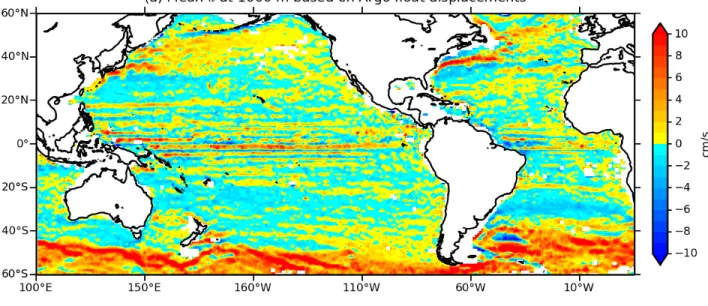
A second scenario for producing EICs over a long zonal extent has been proposed by Ascaniet al. (2010). Instead of DEIV being generated along the western boundary by instabilities of a DWBC, Ascaniet al. (2010) propose that the DEIV is generated by the instabilities of the upper-ocean equatorial current system, in particular those associated with TIWs (Fig. 4b). As seen in the realistic simulation analyzed by von Schuckmannet al. (2008) and in the observations and realistic simulations reviewed by Ascaniet al. (2010), a large fraction of TIW energy radiates into the deep ocean as a downward- and eastward-propagating beam of monthly-periodic MRG waves. Fig. 3b presents new evidence for this with a map of the mean eddy kinetic energy (EKE) near 1000 m, determined from the meridional velocity component (v) estimated from Argo float displacements (see Ollitrault and Colin de Verdière 2014); because near-equatorialv naturally peaks in the intraseasonal wave band, the plot indicates enhanced DEIV along the equator, especially in the eastern Pacific Ocean and western Atlantic Ocean where the TIW-generated MRG waves are expected (blue frames in Fig. 3b). Ascaniet al. (2010) use surface forcing to generate an idealized beam of MRG waves in their numerical model.

When the MRG waves are weak, a set of Eulerian mean currents resembling the EICs appear but they are confined zonally within the beam and the associated Lagrangian mean currents are everywhere 220

225

230

235

zero; when the MRG waves are strong, the EIC-like Eulerian mean currents are found within and to the west of the beam, extending to the western boundary, and they are associated with non-zero Lagrangian mean currents⁴.

The dynamical interpretation of these results given by Ascaniet al. (2010) differs substantially from Huaet al. (2008)'s theory. Ascaniet al. (2010) identified two types of wave instability. The first instability is theself-interaction of the MRG waves (a process neglected in Huaet al. 2008) which gives rise to EIC-like currents within the beam (but not outside). Due to the second instability, the MRG waves lose energy to other types of wave; its main role is to cascade the energy of the MRG wave toward small vertical scales where it is dissipated. Unlike in Huaet al. (2008)'s scenario, the dissipation is key here because it alters potential vorticity at depth and enables the EIC-like currents resulting from the self-interaction to extend west of the beam, a process that is dynamically similar to the formation of aβ-plume circulation (Stommel 1982, Pedlosky 1996; Kessleret al. 2003). Under this scenario, the EICs can be found over a very long zonal scale even if the MRG wave activity is itself zonally confined. We should also note that the focus differs between Hua et al. (2008) and Ascaniet al.

(2010); in the former, the focus is on the initial-value problem while, in the latter, it is on the statistically steady state problem. Despite these differences, however, both studies involve a transfer of energy from DEIV to EICs, and this is the fundamental property that we will check while studying the dynamics of EICs in our solutions (section 5.2).

4 Although the distinction between Eulerian and Lagrangian mean of the circulation is dynamically important (and central to understanding the effects of the these currents on the distribution of tracers), the present work is concerned principally with the Eulerian mean. See Ascaniet al. (2010) for a thorough discussion of the Lagrangian mean associated with the EICs.

240

245

250

255

3 Experimental design

Our ocean model is a version of the Parallel Ocean Program (POP 2.0) model (e.g., Maltrud and McClean 2005), extending from 20°S to 20°N and from 58°W to 14°E to approximate the width of the equatorial Atlantic Ocean, and with a flat bottom at 5000 m. Its horizontal resolution is 1/4° in both longitude and latitude and it has 100 levels, with the vertical resolution progressively decreasing from 10 m near the surface to 100 m near the bottom. Horizontal mixing is parameterized by biharmonic viscosity and diffusion with a coefficient of -2×10¹⁰ m⁴/s, and vertical mixing follows the Richardson- number-dependent scheme of Pacanowski and Philander (1981) with a background diffusivity of 10^-5 m²/s. We use a free-slip bottom boundary condition because preliminary experiments showed that quadratic bottom drag with a non-dimensional drag coefficient of 1.225×10^-3 reduces the DEIV barotropic energy by more than half, thereby significantly reducing the energy source for DEC (see section 6.3).

We obtain four solutions (Tab. 2). The first (Solution 1) is obtained in the rectangular basin noted above. It is forced over the whole domain by the zonal and time-averaged winds observed over the Atlantic Ocean from the European Remote Sensing (ERS-1/2) scatterometer product; hence, the wind stress does not vary in longitude and time but has a realistic meridional profile. The second (Solution 2) has the same configuration as Solution 1, except that it is configured with a realistic coastline of the equatorial Atlantic Ocean (but still with vertical walls at the boundaries), and it is forced by the zonally, meridionally and monthly-varying ERS-1/2 wind stress climatology. The first intermediate solution (Solution 1.5) is similar to Solution 1 except that it has a realistic coastline. The second intermediate solution (Solution 1.8) differs from Solution 2 only in having annual-mean winds 260

265

270

275

280

(no annual cycle).

Sponge layers were not used in these simulations. Experiments including sponge layers on the northern and southern boundaries, implementedvia Rayleigh damping, yielded EDJ basin modes but reduced their amplitude by half. This was apparently an indirect effect via reduction of the DEIV, because in the simulations without sponge layers the high vertical mode coastal Kelvin wave energy does not reach the zonal boundaries, so it would be unaffected by sponge layers there.

The simulations are spun up from a state of rest. Temperature is initially horizontally uniform with a vertical profile derived from the observed potential temperature averaged zonally and meridionally within 5° of the equator in the Atlantic (World Ocean Atlas 2001), and surface temperature is relaxed to the climatological mean with a time scale of one month. Salinity is uniform at 35 throughout each simulation, a simplification that is acceptable for our purpose. The integrations span 50 years for Solution 1, 30 years for Solution 2, 9 years for Solution 1.5 and 15 years for Solution 1.8. Five-day averages are archived in all years for Solution 1 and in years 24−29 for Solution 2.

(Five-day averages and snapshots are nearly identical.) One-year means are archived for all years for Solutions 1.5 and 1.8.

4 Model Results

285

290

295

300

In this section, we report relevant aspects of the flow fields of Solutions 1 and 2, describing first their upper-ocean circulation and DEIV (section 4.1) and then their deep zonal currents that resemble the DEC (section 4.2). We continue by presenting evidence that the spatial and temporal structure of the modeled EDJs in Solution 1 matches that of quasi-resonant, low-frequency, baroclinic equatorial basin modes (section 4.3). We conclude with a brief description of the two intermediate solutions (Solutions 1.5 and 1.8) to help to understand the differences between Solutions 1 and 2.

4.1 Upper-ocean circulation and DEIV

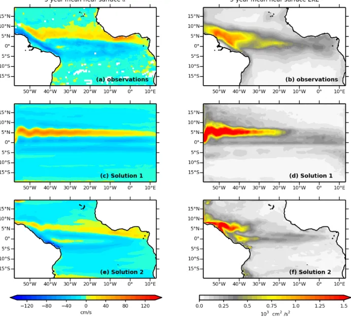
Fig. 5 shows the 5-year mean, near-surface, zonal current and EKE from observations (top panels) and in Solutions 1 and 2 (middle and bottom panels, respectively). The South Equatorial Current (SEC), the North Equatorial Countercurrent (NECC), and a fraction of the North Brazil Current (NBC) are well reproduced in Solution 2 (panel e). In Solution 1 (panel c), the NECC is about 50%

stronger than observed mostly because the zonal width of the basin in Solution 1 is larger than in the observations (see section 4.4). The western boundary current is purely meridional, so there is no zonal component corresponding to the NBC.

The surface EKE field in Solution 2 is overall more realistic than in Solution 1. The high EKE region along the NECC in Solution 2, however, is larger in amplitude but smaller in zonal extent than in the observations. In Solution 1, the high EKE region is stronger and more zonal than in the observations but its zonal extent matches the observations.

The DEIV in Solution 1 (Fig. 6) is similar to that in Solution 2, but stronger in amplitude 305

310

315

320

325

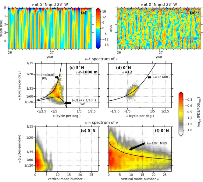
(Fig. 7). It is composed of large-vertical-scale Rossby waves with short periods (30−100 days), moderate meridional scale (~10°) and moderately short zonal wavelengths (5−8°) (Figs. 6c and e).

Near the equator, it includes MRG waves with zonal wavelength of about 8° that are distributed over a range of vertical modes, with higher vertical modes corresponding to lower frequencies (Figs. 6d and f). The increase in small vertical scale energy on the equator is clearly visible in the time series of the meridional velocity component (v) at 23°W, 5°N and 23°W, 0°N (Figs. 6a and b). Based on the analysis of a realistic simulation by von Schuckmannet al. (2008), we conclude that the large-vertical- scale waves of the DEIV correspond to the deep signature of TIWs and are forced by the instability of the upper-ocean circulation. With respect to the moderate- to high-vertical-mode MRG waves at the equator, we will see in section 5.3 that they result instead from the formation mechanism that gives rise to the EDJs.

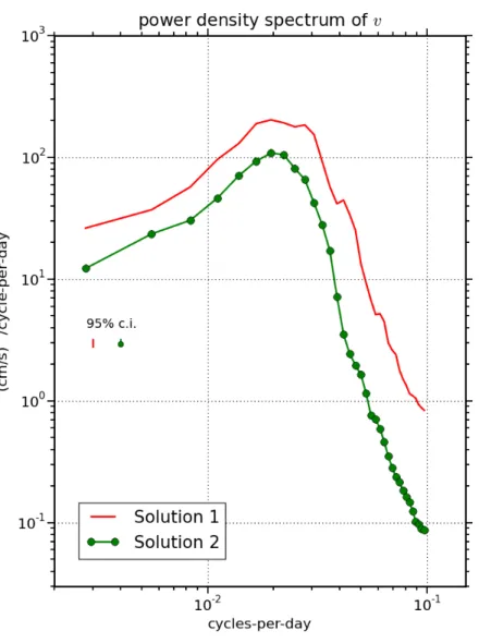
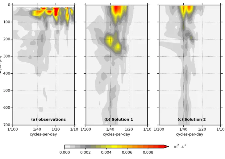
Spectra ofv, zonally- and vertically-averaged along the equator (Fig. 7), are similar in shape for the two solutions, but are weaker by a factor of about 3 in Solution 2, consistent with the weaker upper- ocean circulation in this run (Fig. 5). Using the velocity observations described by von Schuckmannet al. (2008), we compare observed and modeled equatorialv at 23°W using spectra calculated at every available depth between the surface and 700 m (Fig. 8). As already shown by von Schuckmannet al.

(2008; their Fig. 3), there is an increase in DEIV for periods of 20-50 days between 100 and 300 m depth. A similar feature is seen in Solution 2, and a more energetic version appears in Solution 1. In both simulations, the DEIV energy elevation appears to extend deeper than in these observations.

Model-data comparisons of spectra of equatorialv are also performed using four additional datasets:

the velocity measurements described by Bungeet al. (2008) at 23°W between 600 and 1500 m depth and at 10°W between 750 and 1700 m depth as well as the velocity observations collected during the 330

335

340

345

World Ocean Circulation Experiment at 36°W between 3000 and 4000 m depth (Mooring ACM10) and 14.5°W between 1500 and 3000 m depth (Mooring ACM11)⁵. According to these comparisons, the intraseasonal meridional velocity in both simulations appears to be comparable to the observations above about 1500 m depth but is larger than in the observations by a factor of 3-4 below that depth (Fig. 9). Error bars are large, however, so it is not clear which solution reproduces a more realistic DEIV. Note also that both simulations lack energy at lower frequencies, especially at the two easternmost locations.

The Argo-derived meridional velocity components near 1000 m (Fig. 10) provide an estimate of thehorizontal distribution of DEIV energy along the equator. At this depth, Solution 1 reproduces the increase in EKE all along the equator (within 3-4°) although it appears to somewhat overestimate its magnitude. In Solution 2, however, the increase in EKE along the equator is much weaker. Quantitative comparison to Argo is not yet possible, given the available sampling.

In conclusion, it is not clear which of the two solutions reproduces a more realistic DEIV; it might be that Solution 2 is more realistic over the depth range where the DEIV is the largest (upper 300 m; Fig. 8) but less so below at intermediate depths where the DEC is generated. Furthermore, this comparison to observations is hampered by severe undersampling, so that it is restricted to localized comparisons of energy level.

4.2 Deep zonal currents

5-day averages, 6-month averages and 5-year averages of the zonal current along 34°W in the

5 Data along with references can be found at

http://www.nodc.noaa.gov/woce/woce_v3/wocedata_1/cmdac/netcdf/explist.htm.

350

355

360

365

370

simulations are shown in Fig. 11. In both runs, the 5-year mean circulation is dominated by a set of large-vertical-scale flows spanning the whole water column and alternating with latitude. The three flows nearest the equator resemble the EICs described in section 2. They are, however, much more realistic in Solution 1 than in Solution 2: In Solution 1, they attain current speeds of 5−10 cm/s and extend over nearly 40° longitude in the western half of the basin (Fig. 12), consistent with the observations, while in Solution 2 their amplitude is only half as great and they are much less zonally coherent.

The 6-month mean in both solutions has a set of small-vertical-scale currents at the equator (Fig. 11, middle panels). In Solution 1, the set of equatorial currents resembles the observed EDJs, with an amplitude reaching 10 cm/s; the vertical wavelength is about 1000 m, compared to about 600 m in the Atlantic. Consistent with quasi-synoptic observations (Fig. 1), the EDJs in Solution 1 appear also in 5-day averages with an amplitude reaching 20 cm/s (Fig. 11, left panels). In Solution 2, however, the set of equatorial currents does not have a well-defined vertical wavelength and its amplitude reaches only a few cm/s, even in 5-day averages; it is unclear whether this set should be considered as a reasonable, albeit weak, reproduction of the EDJs.

The modeled EDJs in Solution 1 are the most realistic reported so far in the literature, varying in time and depth in a fashion remarkably similar to the observations at 23°W, 0°N (Fig. 2b). Fig. 13 provides a depth-time plot of the low-frequency, zonal velocity (u) at 23°W in Solution 1 (the quantity is scaled and the vertical coordinate stretched with a reference buoyancy frequency of 1 cph;

Gill 1982). Like the observed EDJs, phase propagates downward and their energy upward, with a period of several years. Although both downward and upward energy propagation occurs within the 375

380

385

390

395

first 12 years of the run (not shown), the rest of the simulation is dominated by upward energy propagation, with a modulation at the decadal time scale (Fig. 13).

4.3 Basin modes

In agreement with the observations, the EDJs in Solution 1 have properties consistent with their being the equatorial expressions of quasi-resonant, low-frequency, baroclinic, equatorial basin modes (section 2). The frequency-vertical wavenumber spectrum (Fig. 14) shows that zonal kinetic energy on the equator is concentrated near the basin-mode prediction (1), with a preponderance of upward energy propagation. The lack of symmetry between downward and upward energy propagation suggests that the modes are energized at depth and dissipated nearer the thermocline; the upward-going energy decays to low values before reaching 300 m, and there is little or no energy descending from the 300-m level (Fig. 13). The energy of the basin modes is centered around vertical mode 12 and spans vertical modes 6 to 17. The observed Atlantic EDJs have their energy centered on vertical mode 15 and spread over vertical modes 12 to 20 (Brandtet al. 2008) so that the modeled EDJs in the run with idealized forcing correspond to somewhat larger vertical scales and shorter periods.

The spatio-temporal structure of the low-frequencyu and pressure fields in Solution 1 resembles that of basin modes. The similarity is illustrated in Fig. 15, which presents maps of u associated with upward-propagating energy for the stretched vertical wavelength of 930 m (vertical mode 12) with a resonant period of 3.9 years. To fit the analytical solution from the theory of Cane and Moore (1981) to the numerical one, we used a Rayleigh damping coefficientr(l) = |l|ro, wherero = 2×10^-9 s^-1, which increases linearly with the absolute meridional mode number |l| to mimic the scale- 400

405

410

415

dependent, biharmonic dissipation used in the numerical model⁶. We calculate the solution by summing over all odd meridional mode numbers between -1 and 51; this is a sufficient number of modes as about 90% of the variance is explained solely by the sum of the Kelvin wave (l=−1) and first-meridional mode Rossby wave (l=1). Differences between the numerical and analytical solution occur mainly at 20°W; at this longitude, the meridional width of the pattern is smaller in the analytical solution than in the numerical one, and there are phase differences between the two solutions on and off the equator.

Despite these differences, the comparison in Fig. 15 supports the interpretation of the EDJs in Solution 1 as being the sum of low-frequency baroclinic equatorial basin modes⁷.

In Solution 2, the zonal motion along the equator is dominated by annual and semi-annual waves with low vertical wavenumbers and with net downward propagation of energy (Fig. 14b). The annual peaks occur at wavenumbers consistent with basin modes, as seen in previous numerical studies (Thierryet al. 2004). At lower frequencies, there is a weak local peak of upward-propagating energy that lies on the basin mode dispersion curve, with about the same moderately high vertical wavenumbers (0.9−1.2×10⁻³ cycles-per-meter) and frequencies (1/8−1/2 cycles-per-year) as in Solution 1; however, the signal is no larger than other weak local peaks that are not on the basin-mode curve, consistent with the lack of a clear EDJ signal in the time series of equatorial u of Fig. 2c or in the 6-month mean of Fig. 11e.

6 Although Rayleigh damping is not directly comparable to the Laplacian dissipation used in Greatbatch et al. (2012) to fit a numerical solution of the EDJ-like basin modes to observations, the magnitude of the damping used here appears somewhat weaker. Using Greatbatch et al. (2012)'s notation, if we assume that dissipation in their model is controlled by A∂yy, thenr is equivalent toA/Ly2 whereLy is a meridional scale. WithA=300 m²/s andLy=100 km,A/Ly2 is 3.10⁻⁸ s⁻¹. This discrepancy can be explained in part by the region and the criterion chosen for fitting: here we use three longitudes and compare the shape of theiry-tpatterns while in Greatbatchet al. (2012) the region between 30°W and 15°W is used and the fitting is based on the meridional width of the EDJs.

7 Consistent with this conclusion, we have also checked that little energy is cycling back to the western boundaryvia Kelvin waves along the northern and southern boundaries.

420

425

430

435

4.4 Intermediate solutions

Finally, we conclude with a brief description of the two intermediate Solutions 1.5 and 1.8.

Both are closer to Solution 2 than to Solution 1 indicating that the differences between Solution 1 and 2 are mostly due to the change in coastline rather a change in wind stress.

The upper-ocean circulation in Solutions 1.5 and 1.8 is similar to that in Solution 2 (not shown).

In particular, the maximum speeds of the upper-ocean currents near the western boundary are reduced and reach the realistic level obtained in Solution 2 once a realistic coastline is used. This is because the maximum amplitude of these currents is controlled mostly by the Sverdrup balance and depends on the zonal length over which the wind stress curl is integrated; with a reduced basin in the zonal direction once the realistic coastline is introduced, the maximum speed of the circulation is reduced as well.

Consequently, the upper-ocean circulation is less unstable in the two intermediate solutions compared to Solution 1 and their DEIV has a magnitude similar to that in Solution 2. The DEC in Solutions 1.5 and 1.8 is also similar in shape and amplitude to the DEC in Solution 2 (not shown). One noticeable difference between Solutions 1.5, Solution 1.8 and Solution 2, however, is that the EICs become weaker and less spatially coherent going from Solution 1.5 to Solution 1.8 to Solution 2 (not shown);

this suggests that some aspect of the DEC are sensitive to the zonal structure and annual cycle of the wind stress.

440

445

450

455

5 Dynamical Interpretation

In section 4, we discussed basic properties of Solutions 1 and 2, among other things noting that they contain high-frequency energy (DEIV) and low-frequency structure (DEC). Here, we study the formation mechanism of the most realistic DEC (Solution 1). To do so, we develop an analysis of the zonal kinetic energy budget in the frequency and wavenumber domain, using stretched vertical coordinate (section 5.1). This approach enables us to identify the set of nonlinear interactions among individual waves in the DEIV that produce the LEIC (section 5.2) and EDJs (section 5.3) in Solution 1⁸.

5.1 The zonal kinetic energy budget in frequency-vertical wavenumber space

The zonal momentum equation at the equator is

u_t=−u u_xv u_yw u_z− 1

0

p_xD_H^xD_V^x, (2)

where subscripts represent partial derivatives,u, v, andw are the zonal, meridional and vertical components of the velocity field,p is pressure,ρ0 is a constant reference density, and DHx andDVx are the zonal components of the horizontal and vertical viscous terms, respectively. Following Saltzman (1957), Eq. (2) is Fourier transformed in frequency-vertical wavenumber space:

8 Although the Liouville-Green (also known as WKB) approximation used for scaling and stretching the dynamical quantities is not strictly valid for the large-vertical-scale MRG waves, it is used here simply as a rough scale separation mechanism and does not affect our interpretation concerning the nonlinear interactions.

460

465

470

475

i2 f  u=−u u_xv u_yw u_z− 1

0

p_xD_H^x D_V^x, (3)

where the hat represents the Fourier-transform operator and each quantity is a function of frequency f (in cycles per unit of time), wavenumber m instretched vertical coordinate (in cycles per unit of stretched length), longitudex, and latitudey. We choose to represent the depth-time dependence as exp2im₀zf₀t so thatm0 > 0 andf0 > 0 correspond to adownward phase andupward energy propagating signal. The zonal component of the kinetic energy equation in the frequency-vertical wavenumber space is thus

i2 f  u^*u=− u^*u u_xv u_yw u_z− u^* 1

0

p_xu^*D_H^xu^*D_V^x, (4)

where the asterisk denotes the complex conjugate. The left hand side of Eq. (4) is imaginary, so the real parts of the terms on the right hand side sum to zero with their relative magnitudes indicating how the

“zonal” kinetic energy,u^2, is generated and dissipated (Hayashi, 1982). Calculating these terms for the equatorial slice below 300 m, we find a good numerical balance between the positive and negative contributions in Eq. (4) (Figs. 15a and b, respectively) for all frequencies and vertical wavenumbers. (A weak term, u^*.D_H^x , is not shown.) Next, this energy balance is used to infer the relationships among the DEIV, the LEIC, and the EDJs.

5.2 Linkage of DEIV to LEIC

The LEIC is a time-mean flow with a large vertical scale, so it corresponds to the region of Fig. 16 near zero frequency and zero vertical wavenumber (small square in Fig. 16a). The two terms that perform positive work are the meridional and zonal advective terms (-vuy of Fig. 16a and -uux of 16c, respectively), while the energy loss is mainlyvia the vertical advective term and zonal pressure gradient term (-wuz of Fig. 16d and -px/ρ0 of 16e, respectively). To identify the nonlinear wave 480

485

490

495

500

interactions that contribute to the maintenance of the LEIC against dissipation, we look at all pairs of waves (f1,m1) and (f2,m2) that contribute to the motion at (f0,m0)=(0,0) via the terms -vuyand -uux, where f1+f2=f0 and m1+m2=m0. In the frequency-vertical wavenumber space, that means we look at

−u^*f₀, m₀ vf₁, m₁ u_yf₂, m₂−u^*f₀, m₀ vf₂, m₂ u_yf₁, m₁ (5)

for -vuy, and

−u^* f₀, m₀ uf₁, m₁ u_xf₂, m₂− u^*f₀, m₀ uf₂, m₂ u_xf₁, m₁. (6)

for -uux. Note that, for each expression, the first term is symmetric to the second one with respect to rotation around the point (f0/2,m0/2). For the LEIC, (f0,m0)=(0,0),f1=-f2, m1=-m2, and the two terms in each expression are equal.

Quantities in (5) and (6) for (f0,m0)=(0,0) are plotted in Figs. 17 and 18, respectively. First, we find that the energy transfer via -vuyresults from the interaction of high-frequency waves (mostly short Rossby waves with frequencies from 1/100 to 1/50 cycles-per-day) that are of large vertical scale (Fig. 17). This is consistent with the general mechanism proposed by Huaet al. (2008) and Ascaniet al. (2010), that DEIV is one important source for the EICsvia a transfer of energy from high-frequency waves to the EICs⁹. Second, and quite unexpectedly, we also find an energy transfer from low- frequency baroclinic equatorial basin modes, corresponding to EDJs, to the LEIC via the -uux term (Fig. 18); the interpretation is that each basin mode interacts with itself to transfer energy to the zero-

9 Although in Ascaniet al. (2010), the high-frequency waves involved in the transfer have a vertical wavelength (~1700 m) smaller than those involved here, the transfer is not dependent on this vertical scale as the self-interaction of a wave field of any vertical wavelength produces a large-vertical-scale mean flow.

505

510

515

520

frequency and zero-vertical-wavenumber component that corresponds to the LEIC. To check this result, we calculate the same work but in physical space, that is,

U^EIC.〈−u^EDJu_x^EDJ〉, (7)

whereU^EIC is the time-mean zonal velocity vertically averaged below 300 m,u^EDJ is the zonal velocity field associated with one particular basin mode, (shown in Fig. 15) and the angle brackets indicate a time and vertical mean. In the western half of the basin, quantity (7) is positive on the equator and negative 2° on either side of it (Fig. 19) confirming that the EDJs tend to accelerate the LEIC (consistent with Fig. 18) and decelerate the NICC and SICC. This suggests that, in the statistically steady state, the transfer of energy that maintains the EICs is more complex than initially described by Huaet al. (2008) and Ascaniet al. (2010) and involves not only a transfer from high- to low-frequency components but also between low-frequency components.

5.3 Linkage of DEIV to EDJs

All motions corresponding to the EDJs (dotted lines in Fig. 16) are maintained solelyvia the meridional advective term-vuy, while energy loss isvia the zonal advective term, the zonal pressure gradient term and the vertical friction term (-uux of Fig. 16c, -px/ρ0of 16e andD_V^x of 16f, respectively).

As for the LEIC, we identify the pairs of waves that contribute to a specific basin mode (f0,m0)via the term-vuy using expression (5), but two additional steps are performed initially. In the first step, we distinguish between the eastward- (Kelvin wave) and westward-propagating (long Rossby wave) components of the basin mode. Hence, the contribution to the Kelvin-wave component of the basin 525

530

535

540

mode is

−u^*f₀, m₀; E vf₁, m₁ u_yf₂, m₂−u^*f₀, m₀; E vf₂, m₂ u_yf₁, m₁, (8)

and that to the Rossby-wave component of the basin mode is

−^u^*(f₀, m₀; W) ^v(f₁, m₁) ^u_y(f₂, m₂)− ^u^*(f₀, m₀;W) ^v(f₂, m₂) ^u_y(f₁, m₁), (9)

where qf_i, m_i; E andqf_i, m_i;W are the Fourier components ofq at the frequency fi and vertical wavenumbermi with eastward (E) and westward (W) phase propagation, respectively. In the second step, we focus on wave pairs composed of waves with westward-propagating phase only; this reduces the noise in the calculation without changing the pattern. Hence, quantities (8) and (9) become (10) and (11), respectively:

(10)

and

(11)

Quantities (10) and (11) are plotted in Fig. 20 for the (upward-energy) basin mode with m0=1/645 cycles-per-meter and the associated resonant frequencyf0=1/5.5 cycles-per-year (circle symbol in Fig. 16a); results are qualitatively similar for other upward-energy basin modes. The plot

−u^*f0, m0;W vf1, m1;W uyf2, m2;W−u^*f0, m0;W vf2, m2;W uyf1, m1;W.

−u^*f₀, m₀; Evf₁, m₁;W u_yf₂, m₂;W−u^*f₀, m₀; E vf₂, m₂;Wu_yf₁, m₁;W, 545

550

555

560

demonstrates that the (f0,m0) motion is generated (red/yellow regions) from pairs of MRG waves that range in frequency from 1/100 to 1/30 cycles-per-day, with one wave having a low vertical wavenumber and the other having a vertical wavenumber close tom0.; these are the two types of high- frequency waves that were described in section 4.1 and Fig 6. Note that the intraseasonal high-vertical- wavenumber energy arisesin situ as part of the interactions, while the low-vertical-wavenumber energy corresponds to TIWs and arises from remote instability of surface equatorial currents¹⁰. Further, the interactions between the two types of high-frequency waves contribute to both the Kelvin- and Rossby- wave components of the basin mode, with the interaction for the latter being somewhat stronger.

The aforementioned properties are generally consistent with the theory of Hua et al. (2008) for the EDJs. One difference, however, is that Huaet al. (2008) found that a MRG wave with a specific period gives rise to the EDJs at a specific vertical wavenumber, whereas in our solution all MRG waves (from 30 to 100-day period) participate in the generation of any specified vertical mode. Another is that in Huaet al. (2008), MRG destabilization only generates the Kelvin-wave component of high vertical mode basin modes, whereas we find that, here, it energizes both the Kelvin- and long-Rossby-wave components. Hence, as for EICs, the nonlinear transfer of energy toward EDJs in the statistically steady state appears to be more complex than the transfer described in the initial-value problem studied by Hua et al. (2008).

To address the issue of the asymmetry between upward- and downward-energy basin modes, we repeated the above analysis but for a downward-energy basin mode. Quantities (10) and (11) are found weaker by an order of magnitude than in the upward-energy case over all frequencies and vertical wavenumbers (not shown). This likely results from the weakness of the downward-energy

10 In the ocean, intraseasonal high-vertical-wavenumber energy also arises directly from the instability of the surface equatorial currents (e.g. von Schuckmann et al. 2008) but this is somewhat underestimated in our model.

565

570

575

580

basin mode itself and, unfortunately, does not provide an explanation of why this is the case.

Finally, and for completeness, we also looked at the pair of waves that contribute to the dissipation of the (upward-energy) EDJs via the term -uux. In contrast with the LEIC case, however, we found no pattern in the frequency-vertical wavenumber space (not shown).

6 Conclusions

6.1 Summary

The present study is an attempt to reproduce the DEC in a more realistic setting than in previous studies. In particular, instead of directly exciting a particular set of intraseasonal waves, the approach followed here is to let these waves arise from the instabilities of the large-scale circulation.

The DEC obtained in Solution 1 (rectangular basin and steady wind forcing) has some realistic features. In particular, the EICs extend over a large zonal portion of the basin while the EDJs form low- frequency quasi-resonant equatorial basin modes with energy propagating upward, consistent with the observations.

Further analyses of this simulation confirm the conclusion of previous studies that the DEC 585

590

595

600

results from the rectification of DEIV. In particular, we show that the maintenance of both the EDJs and the EICs is consistent with the instability and nonlinear modification of intraseasonal MRG and Rossby waves, as discussed by previous investigators (d'Orgevilleet al. 2007; Hua et al. 2008;

Ménesguenet al. 2009; Ascaniet al. 2010). We still do not know, however, the cause for the energy difference between upward- and downward-energy EDJs. Finally, we find that EDJs contribute to the maintenance of the EICs, suggesting that the nonlinear transfer of energy in the statistically steady state is more complex than has been described previously.

A puzzling aspect of our study is that the DEC in Solution 2, with more realistic coastlines and wind forcing, is less realistic than in Solution 1. Intermediate solutions 1.5 and 1.8 show that the primary factor is the reduction in basin width when coastlines are added. This reduces the speeds and instability of the upper ocean currents, weakening the DEIV, hence leading to a weaker DEC.

6.2 What can we conclude concerning the modeling of DEC?

The DEC is the end result of a series of complex dynamical processes, some being nonlinear in nature: The mean upper-ocean circulation and deep western boundary currents near the equator give rise to instabilities that generate intraseasonal variability; some of that intraseasonal variability propagates away from its source as equatorial waves which then rectify into the mean and slowly varying DEC (Fig. 4). Hence, for a model to reproduce a realistic DEC, it needs to handle correctly each of these steps, any of which can be impaired by the model's deficiencies, such as a lack of spatial resolution, inadequate forcing, or unrealistic parameterization of subgrid-scale processes.

605

610

615

620

625

For the present solutions, the degree of realism of the DEC appears to depend critically on the amplitude and structure of the DEIV. Hence, we speculate that the model's limitations affect (1) the transfer of energy from the upper ocean to the DEIV and/or (2) the transfer of energy from the DEIV to the DEC.

Unfortunately, observations of the DEIV are inadequate for evaluating the DEIV in simulations.

As concluded in section 4.1, it is not clear which of our two solutions reproduces the more realistic DEIV. Although the DEIV in Solution 1 may be too energetic over the depth range where it is the strongest (upper 300 m; Fig. 8), it may be more realistic than in Solution 2 at intermediate depths, where the rectification into the DEC is most evident (Fig. 10). Indeed, there is one reason to believe that the deeper DEIV in Solution 1 may be more realistic than in Solution 2: von Schuckmann et al.

(2008) noticed that the modeled DEIV energy can increase by a factor of 2 to 3 when using a daily rather than a climatological wind forcing. Hence, the unrealistically strong upper-ocean circulation and instabilities of Solution 1 might compensate for the absence of intraseasonal and higher frequency wind forcing and produce a more realistic deeper energy level for the DEIV compared to Solution 2.

Together with more observations of the DEIV, an additional simulation similar to Solution 2 but with daily wind forcing would test this interpretation.

Alternatively, the DEIV might be closer to reality in Solution 2 than in Solution 1. In this case, the superior DEC representation in Solution 1 might result from a cancellation of errors: perhaps deficiencies in the model's physics weaken the energy transfer from the DEIV to the DEC, and this is compensated by forcing an unrealistically strong DEIV. Indeed, there are three points supporting this interpretation. First, we know that in a model of a wide basin such as the Pacific, DEIV momentum 630

635

640

645

650

dissipation is essential for the EICs to extend westward from their origin (Ascaniet al. 2010), suggesting that it has to be well parameterized for EICs to have a realistic zonal extent. Second, the DEC is weak or non-existent when horizontal Laplacian friction/diffusion and/or half the horizontal resolution (0.5° resolution) is used (not shown), suggesting again that the modeled DEC is sensitive to choices in spatial resolution and subgrid-scale parameterizations. Third, OGCMs have consistently under-estimated the DEC, even when driven with current best estimates of the wind field, and when performing quite well in simulating the upper ocean circulation (Ascani 2005). Additional simulations to study the sensitivity of the energy transfer from DEIV to DEC to a model's resolution and parameters would be needed to confirm this interpretation.

6.3 Effect of bottom friction

During the course of performing these experiments, we found that a quadratic bottom drag with a non-dimensional drag coefficient about half the typical value (1.225×10^-3 versus 2.5×10^-3) damps dramatically both the DEIV and the DEC (not shown). This is again consistent with the conclusion that DEIV is the source for the DEC in the simulations and it may explain in part why the DEC is absent in some existing OGCMs. This hypothesis, however, is at odds with previous studies showing that a moderately strong bottom friction is needed to reproduce a realistic level of EKE in OGCMs (Arbic et al. 2009).

6.4 Additional issues

Other issues have not been addressed in the present study. First, bottom topography is not 655

660

665

670

included in any of our simulations; given that even simple parameterized bottom friction was found to reduce DEIV and DEC and was therefore omitted, we expect the roughness and blocking effects of the Mid-Atlantic Ridge must be important for the DEIV and the DEC. Second, it is unclear whether the zonal jets found poleward of the EICs (e.g. Qiuet al. 2013) are dynamically similar to the EICs.

Finally, we have not studied the Lagrangian transport associated with the time-varying DEC, which affects the zonal distribution of biogeochemical properties (Getzlaff and Dietze 2013; Dietze and Lopetien 2013). This transport is a function of the model dissipation (Ascani et al. 2010) and the analysis of the Lagrangian component of the DEC as a function of subgrid-scale parameterization, in a model capable of simulating a realistic DEC, would be needed to address this important issue.

675

680

Acknowledgements

We dedicate this paper to the memory of Bach Lien Hua, who contributed so much to the understanding of the dynamics of the EDJs and EICs. We thank Dailin Wang who actively contributed to the first phase of this study and to Christine Provost and Lucia Bunge who kindly shared their velocity data with us. We also thank the two anonymous reviewers for their constructive comments.

The surface drifter climatology of ocean currents has been developed by NOAA/AOML/PMEL and can be found athttp://www.aoml.noaa.gov/phod/dac/dac_meanvel.php. The YoMaHa product is developed by the International Pacific Research Center (IPRC) at the University of Hawaii and is available athttp://apdrc.soest.hawaii.edu/projects/Argo/index.php. This work was funded in part by NSF Grant OCE0327334 (FA and EF), the IPRC (FA), the German Science Foundation as part of the Sonderforschungsbereich 754 “Climate-Biogeochemistry Interactions in the Tropical Ocean” and by the German Federal Ministry of Education and Research Grant 03F0651B (PB and RJG). PB and RJG are also grateful for continuing support from GEOMAR. Moored velocity observations at the equator were acquired in cooperation with the Prediction and Research Moored Array in the Tropical Atlantic (PIRATA) project. IPRC contribution #### and SOEST contribution ####.

685

690

695

700

References

Arbic, B. K., J. F. Shriver, P. J. Hogan, H. E. Hurlburt, J. L. McClean, E. J. Metzger, R. B. Scott, A.

Sen, O. M. Smedstad, and A. J. Wallcraft, 2009: Estimates of bottom flows and bottom boundary layer dissipation of the oceanic general circulation from global high-resolution models. J. Geophys.

Res., 114, doi:10.1029/2008JC005072

Ascani, F., 2005: The equatorial subthermocline circulation in ocean general circulation models. M.S.

Thesis, University of Hawaii at Manoa, 67 pp.

Ascani, F., E. Firing, P. Dutrieux, J. P. McCreary, and A. Ishida, 2010: Deep equatorial ocean circulation induced by a forced-dissipated Yanai beam.J. Phys. Oceanogr., 40, 1118–1142, doi:10.1175/2010JPO4356.1

Bourlès, B., M. d'Orgeville, G. Eldin, Y. Gouriou, R. Chuchla, Y. du Penhoat, and S. Arnault, 2002:

On the evolution of the thermocline and subthermocline eastward currents in the Equatorial Atlantic. Geophys. Res. Lett., 29, doi:10.1029/2002GL015098

Bourlès, B., and Coauthors, 2003: The deep currents in the eastern equatorial Atlantic Ocean. Geophys.

Res. Lett., 30, doi:10.1029/2002GL015095

Brandt, P., V. Hormann, B. Bourlès, J. Fischer, F. A. Schott, L. Stramma, and M. Dengler, 2008:

Oxygen tongues and zonal currents in the equatorial Atlantic. J. Geophys. Res., 113, doi:10.1029/2007JC004435

Brandt, P., A. Funk, V. Hormann, M. Dengler, R. J. Greatbatch, and J. M. Toole, 2011: Interannual atmospheric variability forced by the deep equatorial Atlantic Ocean.Nature, 473, 497501, doi:

10.1038/nature10013

Brandt, P., and Coauthors, 2012: Ventilation of the equatorial Atlantic by the equatorial deep jets. J.

705

710

715

720

725