A Small Continuous Time Macro-Econometric Model of the Czech Republic

A Small Continuous Time Macro-Econometric Model of the Czech Republic

Emil Stavrev

Transition Economics Series

A Small Continuous Time Macro- Econometric Model of

the Czech Republic

Emil Stavrev July 2000

Transition Economics Series

Institut für Höhere Studien (IHS), Wien Institute for Advanced Studies, Vienna

Contact:

Emil Stavrev Czech National Bank Economic Modelling Division Na Prikope 28

115 03 Prague 1, Czech Republic email: Emil.Stavrev@cnb.cz

Founded in 1963 by two prominent Austrians living in exile – the sociologist Paul F. Lazarsfeld and the economist Oskar Morgenstern – with the financial support from the Ford Foundation, the Austrian Federal Ministry of Education and the City of Vienna, the Institute for Advanced Studies (IHS) is the first institution for postgraduate education and research in economics and the social sciences in Austria. The Transition Economics Series presents research done at the Department of Transition Economics and aims to share “work in progress” in a timely way before formal publication. As usual, authors bear full responsibility for the content of their contributions.

Das Institut für Höhere Studien (IHS) wurde im Jahr 1963 von zwei prominenten Exilösterreichern – dem Soziologen Paul F. Lazarsfeld und dem Ökonomen Oskar Morgenstern – mit Hilfe der Ford- Stiftung, des Österreichischen Bundesministeriums für Unterricht und der Stadt Wien gegründet und ist somit die erste nachuniversitäre Lehr- und Forschungsstätte für die Sozial- und Wirtschafts- wissenschaften in Österreich. Die Reihe Transformationsökonomie bietet Einblick in die Forschungsarbeit der Abteilung für Transformationsökonomie und verfolgt das Ziel, abteilungsinterne Diskussionsbeiträge einer breiteren fachinternen Öffentlichkeit zugänglich zu machen. Die inhaltliche Verantwortung für die veröffentlichten Beiträge liegt bei den Autoren und Autorinnen.

illustrate how the model can be used to determine the nominal equilibrium exchange rate of the Czech koruna in a macro-economic framework. The paper also investigates the effectiveness of monetary and fiscal policies in the presence of a fixed exchange rate regime and massive capital inflows. The search for an equilibrium point is outlined and stability and sensitivity analyses are provided, along with in-sample static and dynamic predictions with the approximate discrete analogue.

Keywords

Macro-econometric model, nominal equilibrium exchange rate, effectiveness of monetary and fiscal policies

JEL Classifications

C51, C52, C53, E17, E50

Comments

This research was undertaken with support from the European Union’s Phare ACE Programme 1996.

I would like to thank Prof. S. Reynolds, Assistant Prof. E. Koèenda, Prof. R. Filer, Prof. J. Kmenta, Prof.

A. Wörgötter, and my colleagues at the Centre for Economic Research and Graduate Education, and the Institute for Advanced Studies in Vienna for many helpful comments. All errors, however, are mine.

1. Introduction 1

2. Theoretical Framework 2

2.1. Qualitative Analysis of the Model ... 3

2.1.1. Search for an Equilibrium Point ... 3

2.1.2. Stability of the Model ... 4

2.1.3. Sensitivity of the Model ... 5

3. Specification of the Model 5 4. Econometric Results 11 4.1. Estimated Parameters ... 14

4.2. Stability and Sensitivity ... 16

4.3. Results for the In-Sample Predictions... 17

4.4. Calculation of the Equilibrium Nominal Exchange Rate ... 20

4.5. Effectiveness of Monetary and Fiscal Policies ... 21

4.5.1. Scenario 1 ... 21

4.5.2. Scenario 2 ... 22

5. Conclusions 24

References 25

Appendix 1. Derivation of the Approximate Discrete Analogue 27 Appendix 2. Search for an Equilibrium Point and Linearization

Around It 31

Appendix 3. Data Description 37

1. Introduction

Over the past seven years the Czech Republic has undergone significant reforms in its transition toward a market economy. At the beginning of these market reforms, the Czech Republic introduced a fixed exchange rate regime which helped to stabilize the macro- economic situation in the Czech Republic. At the beginning of the transformation the country experienced a relatively high decline in real GDP (14.2% for 1991 and 6.4% for 1992) which was halted in 1993. However, the economy recovered in 1994 when growth was 2.6%.

Economic growth reached 5.5% in 1995, which was the maximum growth rate for the past seven years. In 1996 and 1997 the growth rates were 4.1% and 1.7% respectively (see Nachtigal [1997] and Hajek et al. [1997a and 1997b]). Following a major price deregulation in 1991, the average yearly inflation rate reached 56.6% in 1991 and then fell to 11.1% in the following year. The main reason for the jump in the inflation rate to 20.8% in 1993 was the introduction of a VAT and a second big deregulation of prices at the beginning of the year. In the following years the average inflation rate was below 10%.

The fact that the Czech Republic’s economy recovered relatively quickly and the inflation rate dropped to below two digits in a three-year period helped to attract foreign investment, which totaled around 8.4 billion USD at the end of 1998. Since 1994 the country has registered a current account deficit, which gradually increased from 3% in 1994 to 7.6% for 1996 and to 8.7% for the first quarter of 1997, although it subsequently fell during the last three quarters of 1997 to 6.1% at the end of the year and is expected to reach 1.4% for 1998. The huge capital inflows and the current account deficit have caused problems for policy-makers. In the presence of a fixed exchange rate regime, capital inflows had an inflationary impact and the increasing current account deficit has caused devaluationary expectations for the Czech currency.

Even though the country is in transition and has a short time series, it is interesting to look at the relationship among different macro-economic variables on one hand and the possibility of influencing their evolution over time by policy-makers. To date few macro-econometric models for the Czech Republic have been published; J. L. Brillet and K. Šmidková (1997) presented a medium-sized macro model of the Czech Republic aimed at capturing the specific characteristics of a transition economy. The macroeconomic impact of the transition process and the effect of external factors on macro-economic variables are investigated in Šujan and Šujanová, (1995). A Bayesian approach and the application of a Kalman filter in the estimation of a macro-econometric model of the Czech Republic are developed in Vašièek (1997).

The aim of this work is to estimate a relatively small continuous time macro-econometric model, which can later be used for the following purposes. Firstly, to determine the impact of the policy parameters on the nominal equilibrium exchange rate of the Czech koruna in the context of a macro-dynamic framework. Secondly, to predict the values of the nominal

exchange rate. Thirdly, to investigate the effectiveness of monetary and fiscal policies as applied to the Czech Republic.¹

We use continuous time models because they have several attractive properties. These types of models are small and thus easy to manipulate analytically, which represent advantages over the large macro-econometric models where the properties of the model are investigated using numerical simulations. A continuous time model may also allow a more satisfactory treatment of distributed lag processes. An additional advantage is that these models allow for a better treatment of mixed flow-stock variables usually present in macro- econometric models. They take into account the fact that a flow variable is not measured instantaneously and that what one observes is in fact its integral over a certain period. Lastly, these models in principle ought to have an equilibrium, but it is important to note that this does not mean that the model is in this kind of equilibrium or that the equilibrium is necessarily stable. Therefore, the model can be solved for the actual paths, which may or may not be the equilibrium path.² This property seems especially attractive in modeling the economies of countries in transition.

The rest of the paper is organized as follows. In Section 2 we present the theoretical framework used to construct the model. In Section 3 the specification of the different equations of the model is given. Section 4 presents econometric results and analysis stability and sensitivity of the model. In this section we suggest a way to calculate the nominal equilibrium exchange rate and investigate the effectiveness of monetary and fiscal policies.

Section 5 concludes.

2. Theoretical Framework

The theoretical base used in this work follows the principles explained in several works written by Gandolfo, Bergstrom and Wymer.³ In general the process of adjustment to excess demand can be formulated mathematically as:

Dy(t) = f (x(t) - u(t)), (1)

1 It should be mentioned that the purposes for which the model can be used are not by any means restricted to the ones described above. After incorporating interest rates into the model it will be possible to use it to predict inflation.

Hence, it can become a very useful tool for the purposes of inflation targeting, a policy adopted by the CNB at the beginning of 1998.

In its present version the model is constructed under the assumption of a fixed exchange rate regime. It is possible, however, provided that longer time series are available, to change the model in such a way so as to account for the change in the exchange rate regime in mid-1997. We believe that even in this version the model is useful for performing simulations which can be of interest not only for the Czech Republic, but also for other countries (Estonia, for example) which have fixed exchange rate regimes.

2 For the construction and estimation of a continuous time disequilibrium model of the UK financial market see Wymer (1973).

3 For complete and detailed explanations of the matter see Gandolfo, G. (1981) and Bergstrom, A. (1990).

where D denotes the differential operator d/dt and f is a sign-preserving function, satisfying the conditions f (0) = 0 and f ^’(0) > 0. One obtains a partial adjustment equation in the strict sense when x(t) = y t$( ) and u(t) = y(t). If x(t) and u(t) are functions of other variables, then variable y(t) adjusts in relation to the difference between the desired and actual values of these variables.

Further, equation (1) will be linearised around the sample mean or the equilibrium point to obtain:

Dlny(t) = α(lnx(t) - lnu(t)). (2)

On the basis of the above formulations, the model can be written as a first order differential system in the normal form as follows:

DlnX(t) = F[lnX(t),Z(t),θ] + ε(t), (3)

where X(t) is a vector of endogenous variables, Z(t) a vector of exogenous variables, θ a vector of parameters, F a vector of linear or non-linear differentiable functions, and ε(t) a vector of disturbances with classic properties. The vector of parameters θ consists of the speed of adjustment parameters − α, constants or propensities − γ, elasticities − β and policy parameters − δ. For simplicity, later in this section ε(t) is omitted. The disturbances will be dealt with again in Section 4.

2.1. Qualitative Analysis of the Model

We perform a qualitative analysis of the model using methods from mathematical economics. In order to investigate the general properties of the model we: 1) search for an equilibrium point; 2) examine its stability; and 3) perform analysis of sensitivity.

2.1.1. Search for an Equilibrium Point

In order to find an equilibrium point, the method of undetermined coefficients will be applied.

Exogenous variables are assumed to grow at a constant proportional rate,

Zi(t) = Z^*i e ^{λi t},for all i, (4)

where Z^*i are the initial levels of the exogenous variables and λi the growth rates.

The equilibrium solution is given as a particular solution of the system (3) in the following form:

Xi(t) = Xi

* e ^{ρi t}, for all i, (5)

where the values of Xi* and ρi must be determined. The equilibrium point levels Xi*

depend on the initial levels of the exogenous variables, the growth rates and the parameters of the model. The growth rates of the equilibrium paths of the endogenous variables, ρi,, depend on the exogenous growth rates and the sub-vector of parameter vector θ. Parameter vector θ includes elasticities and the propensity to consume, but not the speed of adjustment parameters. Formally, if θ = {α,β}, where α is a sub-vector of adjustment parameters and β is a sub-vector of propensities and elasticities, then it follows that

ρ = φ1(λ,β) (6)

X^* = φ2(Z^*,λ,θ). (7)

We provide a detailed description of the method along with the solutions for the equilibrium point in Appendix 2.

2.1.2. Stability of the Model

We will deal with the local stability of the system (3) in this section. In order to ascertain whether the system (3) is locally stable or not, we linearise it around the equilibrium point, using Taylor series expansion and neglecting all higher order terms. The original system (3) explicitly contains functions of time and, thus, it is not an autonomous system. In this case one must define the conditions under which one may neglect the higher order terms in the Taylor series expansion. Let us consider the following system:

Dx(t) = Ax(t) + f(x,t) (8)

The null solution x(t) = 0 of the system (8), where A is a matrix of constants, is asymptotically stable if ||f(x,t)||/||x|| tends to zero uniformly in t as ||x|| tends to zero and A has characteristic roots with negative real parts. If the above condition is satisfied then the system below is called a uniformly good approximation of the original system (3):

Dx(t) = Ax(t) (8’)

The system (8’) will be asymptotically stable if, and only if, all characteristic roots of the matrix A have negative real parts.

One important feature of continuous time models is that for most of them the original system is autonomous (time is not explicitly present in them), which means that after linearization around the equilibrium point, one obtains a system that is a uniformly good approximation of the original system. It is an important characteristic because the question of uniform convergence then does not arise, and in order to investigate the stability of the model it suffices to focus on the linearised system or precisely on the characteristic roots of the

matrix A. The original system is locally stable if all the characteristic roots of the matrix A have negative real parts. The stability analysis for the estimated model is given in Section 4 below.

2.1.3. Sensitivity of the Model

In the sensitivity analysis, we compute the partial derivatives of the characteristic roots with respect to the parameters. This analysis is particularly useful for examining dynamic behavior and the policy implications of the model. This allows us to evaluate the effect of a change in any one of the parameters in the model, and especially policy parameters on the dynamic properties of the system, without having to use numerical simulations. The characteristic roots of matrix A are functions of its elements and these elements are functions of the parameters of the model. Hence, one can examine the effects of changes in the parameters of the estimated model on the characteristic roots by computing the partial derivatives of the eigenvalues with respect to the parameters. The above definition of sensitivity analysis is developed in Wymer (1976) and Bergstrom (1990). The results of the sensitivity analysis for the estimated model are presented in Section 4 below.

3. Specification of the Model

The model is an interdependent system of stochastic differential equations specified according to the theoretical base discussed in Section 2. To simplify, the disturbance terms are omitted. The symbol (^) refers to the partial equilibrium level, or the desired value of the variable, (^e) to its expectation, and ln to the natural logarithm. All parameters are assumed to be positive unless otherwise specified.

Consumption function

DlnC = α1ln

C$ C



 

 + α2 m2 (9)

where

C$ _{= γ}1 Y where γ1 is marginal propensity to consume (9.1)

C − real consumption (both private and government) m2 − proportional rate of change of money supply (M2) Y − real gross domestic product

In equation (9) real aggregate consumption⁴, C, adjusts to its desired level, C$, which is given as the marginal propensity to consume applied to real domestic income.⁵ The second term in this equation must capture the impact of the monetary variables, proxied by m2, on consumption. The above specification is similar to the one specified in Hendry and Ungern- Sternberg (1981) and differs from the consumption functions discussed in Whiteley (1994) by not including inflation as a proxy for the inflation loss on liquid assets. The idea is that nominal money balances play a buffer role in the private sector asset portfolio, allowing unexpected variations in income and expenditure.

Imports

DlnIm = α3 ln

$Im Im



 

 + α4 ln

V$ V



 

 (10)

where

Im$ _{= γ2} P P_f



 



β1

(DK) ^β2 C^β3 E^β4 (10.1)

V$ _{= γ}4Y ^e, (10.2)

Im − real imports

V − stock of inventories in real terms

DK − change of fixed capital stock in real terms E − real exports

P − domestic price level (CPI) Pf − foreign price level

Real imports defined in equation (10) are determined by two terms. First, they adjust to their desired value Im$ , which is a function of terms of trade, investment, consumption, and exports all in real terms. This specification connects demand for imports to total sales and takes into account the fact that some imported goods are included in exports. Second,

4 Precisely speaking, in equation (2.9) and in the following equations we define the rate of change in the left hand side variables as opposed to their real levels, but after the integration of the system (2.9) − (2.20) we will obtain the levels of the variables.

5 Because C is total consumption, private plus public, we may use the net of depreciation GDP instead of the net disposable income.

imports are connected to the change in inventories. If inventories are less than their desired level, imports will increase. Hence, inventories are supposed to play a buffer role between supply and demand in the goods market.

Exports

DlnE = α5 ln

E$ E



 

 (11)

where

E$ _{= γ3P}^−β5_e^λ1t _(11.1)

t − time

Equation (11) defines the demand for real exports of goods and services. Their partial equilibrium level depends on the price level and a trend term, which accounts for the change in foreign demand for exports and foreign price level. The parameter λ1 can be considered a weighted sum of the growth rates of real income and price level in the rest of the world.⁶ This specification has some advantages over the usual export demand specification where terms of trade and foreign income explicitly determine the desired level of exports (for example, a variation in the exchange rate is allowed by changing the parameter γ3).

Expected output

DlnY ^e = ξ ln Y Y^e



 

 ⁽¹²⁾

Y ^e − expected output

Equation (12) defines expected output. Expected output evolves according to an adaptive expectation mechanism and has two functions in the model. In addition to determining real output, it connects real output to the rest of the model by the presence of the second term in equation (13) below.

6 For the estimation we use the price level in the rest of the world, which is constructed as a weighted average of US and German price levels as follows: Pf = 0 .35*eDM$* Pus + 0.65*PGer where eDM$ is the exchange rate of the US dollar with respect to German mark. Thus, the price index for rest of the world is expressed in German marks. We obtain income for the rest of the world in the same way.

Instead of the traditional specification of the export function we use the one above because we believe that in a period of changing structure of exports and fighting for market shares in western countries the impact of the real exchange rate on exporters will not be a major factor in their exports. The specification used here is thought to better capture the process of conquering new markets, which may contradict exchange rate developments.

Output⁷

DlnY = α6 ln Y Y

 e

 

 ^{+ α7 ln} V$ V



 

 (13)

where

V$ _{= γ}4Y ^e. (13.1)

Real output is defined in equation (13). It adjusts to its desired level, which in this case is represented by expected income and depends on the difference between the desired level of inventories and their actual level. It is assumed that producers have a desired ratio of inventories to expected output − γ4. Hence, they will increase output and imports when the desired inventories are bigger than the actual inventories.

Fixed capital formation

Dk = α8{ DK K

 $

 

- k} + α9 m2 (14)

where

DK$ _{= γ}

5Y ^e (14.1)

Equation (14) defines the development of the fixed capital stock. The proportional change of capital stock k adjusts to its desired level k$= DK

K

 $

 

. The desired investment,DK$_{, is a}

function of expected income. As in the consumption function, the speed of the adjustment of k to its desired level is assumed to be an increasing function of m2. The idea is to use the percentage change in M2 as a proxy for the credit conditions in the economy. It may seem more appropriate to use the interest rate in the above equation and incorporate it into the whole model, but we have decided not to include the interest rate for several reasons. First, due to the process of transition and the lack of a developed banking system, the interest rates in the Czech Republic were not set according to the market until the beginning of 1994.

7 Instead of equation (12) for expected output and equation (13) for output it is possible to construct the model using an equation for output of the following type:

D Y C DK E

Y

C DK E

Y V

Y

V

ln ln ( ) V

ln ( )

=  + +

 

 +

+ +



 

α γ 

α γ

(13V) where the sum of C + DK + E equals total sales for consumption, capital formation and exports. We used the specification in the paper in order to evaluate the impact of expectations in the economy.

Second, it seems plausible to assume that, for countries in transition, the interest rate may not be the main factor affecting the investment decisions of the economic agents during the first stage of the transformation.

Domestic price level

DlnP = α¹⁰ ln

P$ P



 

+ α¹¹ ln M M _d

2 2



 

 ⁽¹⁵⁾

where

P$ _{= γ}6Pfβ6 W Pr



 



β7

(15.1)

M2_d = (PY) ^βmd − money demand (15.2)

M2 − nominal stock of money supply Pr − productivity

W − nominal wage

Domestic price level is defined in equation (15). In the first term domestic price level adjusts according to the difference between the desired and actual price level. The desired price level is assumed to depend on both domestic and foreign factors. The domestic cost factors are represented by the level of the nominal wage rate W and of productivity, which is exogenously given. The foreign factor is represented by the foreign price level. The second term represents the monetary factor in determining domestic price level. The fact that money supply is not included in the partial equilibrium level of P is in accordance with the monetarist approach and simply shows that the adjustment of the price level is not constant.

Wages

DlnW = α12 ln

W$ W



 

 (16)

where

W$ _{= γ}7 P^β8 e^{λ2 t} (16.1)

The nominal wage rate, equation (16), adjusts to a partial equilibrium level W$ , which depends on the domestic price level and institutional factors (trade unions, etc.). Thus, it is assumed that the target nominal wage exceeds the level determined only by the domestic price level. The institutional factors are captured by the trend term in the formula for the desired nominal wage.

Influence of the Balance of Payments on Money Supply

Dm2 = α13 (m$_{2 - m2)} (17)

where

m$_{2 = δ}1 ln E γ8Im



 

 - δ2 Dln P P_f



 

, δ1 < = > 0, (17.1) Equation (17) is a policy function and describes the monetary authorities’ adjustment of the percentage change of nominal money stock to its target value m$2. The first and the last terms capture the balance of payments effects. The parameter γ7 can be interpreted as the ratio of exports to imports which the monetary authorities aim at in order to attain the desired structure of the balance of payments. The second term in this equation represents the anti- inflationary target of the monetary policy, which in this case focuses on relative price stability.

The δ coefficients represent the different weights given to the different targets. Coefficient δ2

must be positive, while δ1 may be either positive or negative.

Capital Stock

DlnK = k (18)

Money Supply

DlnM2 = m2 (19)

Inventories

DV = Y + Im - E - C - DK (20)

The last three equations in the model are definitions. Equations (18) and (19) help us to express the model as a system of 12 first order differential equations. Equation (20) defines the change in the real inventories as a residual term.

In the model there are twelve equations and twelve endogenous variables. The only exogenous variables in the model are time − t, productivity⁸ − Pr and foreign price level − Pf.

4. Econometric Results

For estimation purposes the approximate discrete analogue is used (for the complete derivation see Gandolfo, G. [1971]). After the linearization of the system (3), one obtains a system of the following type:

Dx(t) = Ax(t) + Bz(t) + ε(t) (21)

We integrate the system (21) over the interval (t - δ, t) using the following approximations:

1

δ∫0^δ Dx t( δ−s ds) ≈^∆x_t , ∫^δx t(δ−s ds) ≈^Γx_t

0

, (22)

where ∆ ≡ 1

δ (1 - L) and Γ ≡ 1

2 (1 + L), L is the lag operator, and δ is the length of the observation interval. If one further assumes the length of the observation interval equal to the basic time unit then δ = 1. Using formulas (22) the system (21) can be written in the following form:

∆xt = AΓ xt + BΓzt + υt , (23)

where υt is a vector of disturbances that depends on ε and on errors of approximation. The new disturbances will be serially uncorrelated only if there are no mixed stock-flow variables.

If the opposite is true, the system (21) must be integrated twice, once to obtain measurable variables and once to obtain the approximate discrete analogue. After the second integration one obtains

∆xt

0 = AΓ xt

0 + BΓzt

0 + ηt (24)

88 In order to endogenise productivity the following equation is estimated:

D W DK

ln Pr . ln ( ) Pr

( . )

. .

( . ) ( . )

= 









 1 02

0 2

0 43 0 08

0 02 0 06

(16.V)

The idea is that the desired level of productivity depends on the nominal wage rate W and investment. Predictions of the model consisting of equations (9) − (20) plus equation (16.V) were not satisfactory and we did not include equation (16.V) in the final version. One possible reason for the less satisfactory results is that the use of aggregate data makes it difficult to distinguish between newly established and old capital, which may lead to underestimating the effect of investment on productivity.

Measurable variables are denoted by superscript (⁰). Let x⁰(t) be a flow variable. The integral

x t^o( )= ¹∫x t( −s ds)

δ ^δ0 δ ⁽²⁵⁾

is measurable and an observation of this integral over the interval (τδ - δ, τδ) is denoted by xt0. In fact, this is what one observes in reality for a flow variable. If xt0

is a stock variable, then the integral (25) is not observable. We evaluate it using the trapezoidal rule. In this case the observation of the integral of a stock variable is approximately given by

xt

0 = Γxt (26)

where Γ is defined above. Let x1(t) denote the instantaneous change of a stock variable and x1(t) = D x(t). We obtain a measurable value for this type of variable from the point observation on the stock variable x(t). After integrating x1(t), we have

x1t0 = ∆xt (27)

where ∆ is defined above and x1t0 is the observation on x1(t).

We transformed the system of differential equations (21) into a system of difference equations by integrating it twice. The process of integration leads to the introduction of autocorrelation. It is possible, however, to derive an approximation of the process of formation of disturbances ηt that is independent of the parameters of the model. This approximation is given by⁹

ηt ≈ (1 + 0.268L)ωt (28)

where ωt is a serially uncorrelated random disturbance. Since the moving average process in (28) is independent of the parameters of the model, we may use the inverse of this process to obtain a model with serially uncorrelated disturbances. Hence, we obtain the following for the uncorrelated disturbances

ωt ≈ (1 + 0.268L)^-1 ηt (29)

Next we expand the term in brackets in (29) in Taylor series to obtain the formulas below, which are used to transform the original variables.

xt

* = xt

0 - 0.268x⁰t-1 + 0.072x⁰t-2 - 0.019x⁰t-3 (30)

9 For complete explanation see Gandolfo, G. (1981) Ch. 3

zt

* = zt

0 - 0.268z⁰t-1 + 0.072z⁰t-2 - 0.019z⁰t-3

where xt0

is a vector of observed endogenous variables and zt0

is a vector of observed exogenous variables. It is obvious from the second equation of (30) that if the vector of exogenous variables contains a constant term, it must be multiplied by 0.785 (which is exactly the sum of the coefficients of the zt0

variables).

Applying the above procedure to the model (23) gives us the final version of the approximate discrete analogue

xt

* - x^*t-1 = A1 2 ( xt

* + x^*t-1) + B1 2( zt

* + z^*t-1) + ωt. (31)

For estimation purposes the following form will be used

(I - A1 2) xt

* = (I + A1

2)x^*t-1 + B1 2 ( zt

* + z^*t-1) + ωt. (32)

Now disturbances ωt are assumed to be uncorrelated.

In order to estimate the system (9) − (20), we first linearised equations (14) and (20) around the sample mean. The linearization and derivation of the approximate discrete analogue are described in Appendix 1.

The system described in Section 3 contains 34 parameters to be estimated. The ideal method to estimate this system would be the full-information maximum likelihood (FIML) method. However, the short data sample (28 quarterly observations for the period from the first quarter 1991 to the fourth quarter of 1997) prevents us from using this or other simultaneous techniques (for example, three stage least squares) to estimate the specified model. We decided to use the two stage least squares method (2SLS) because it handles the case of nonlinearity in both variables and coefficients and, unlike OLS, it also provides consistent estimates if endogenous variables are present in the right hand side of the equations (see Fair [1984]). The relevant instruments for the estimation are as follows. First, we used all predetermined variables in the model as instruments for each structural equation and second, we used all exogenous variables included in the model as instruments.

Concerning the functional form of the instruments we followed the rule that the functional form of the instrument was the same as the functional form of the variable for which this instrument was used. The 2SLS technique, although consistent, is generally not asymptotically efficient because it does not take into account the correlation of the structural disturbances across equations. We are aware of the fact that the ratio of the estimated coefficient to its estimated standard error does not have a t distribution. However, we use the t distribution as a tolerable approximation of the true distribution on the basis of the available

Monte Carlo experiments, which suggest that the distortion is usually reasonably small (see Kmenta [1986], Green [1997]).

4.1. Estimated Parameters

We present the estimated equations below. Standard errors are given in brackets. In the interest of simplicity the error terms are omitted.

DlnC = 1 39

0 17

.

( . )ln

0 72

0 022.

( . )Y C











 ^{+ ( .2 200 94. )m2 (9’)}

DlnIm = 187

0 078

.

( . )ln

1 350 087

1 26

0 41 0 76 0 17

0 55

0 043 0 0

.

Im

( . )

.

. . .

( . )

( . ) ( .116 ) ( .12 )

P

P DK C E

f



 























−

+1 07

0 28

.

( . )ln 0 95

0 12

.

( . )Y V

 e













 (10’)

DlnE = 1 3

0 254

.

( . )ln

187 61

64 15

0 35 0 042

0 0 0155

.

( . )

. .

( .12 ) ( . )

P e E

− t















 ^(11’)

DlnY = 1 96

0 265

.

( . )ln Y Y

 e

 

 + 0 21

0 132

.

( . ) ln 0 95

0 12

.

( . )Y V

 e













 (13’)

Dk = 1 49

0 186

.

( . )

0 264

0 051

.( . ) Y

K k

 e

 

 −











 + 0 243

0 099

.

( . )m2 (14’)

DlnP = 0143

0 072

.

( . )

ln 0 63

0 77 1

0 175

0 361)

. Pr

( . )

.

P W ( .

P

f



























+ 0168

0 082

.

( . )

ln M PY

2 ( )1



 

 (15’)

DlnW = 1 06

0 249

.

( . )ln

5663 25

603 82

0 209 0 039

0 179 0 0048

.

( . )

. .

( . ) ( . )

P e

W

 t













 (16’)

Dm2 = 1 374

0 229.

( . ) {0 068

0 079.

( . )ln E

0 470 413. Im

( . )











 ^{- ( .0 790 992. )Dln} P P_f



 

 ^{- m2}, (17’)}

The speed of adjustment parameters α may be divided into two groups. The first group consists of all α parameters without α2, α4, α7, α9 and α11, and expresses the speed of adjustment of the corresponding variables to their desired or partial equilibrium levels. The second group includes parameters α2, α4, α7, α9 and α11 , which relate the rate of growth of one particular variable to another variable (as is the case with consumption and capital formation) or to the discrepancy between the other variable and its desired or partial equilibrium level (as in the domestic price level equation or the imports equation). Of all the adjustment parameters, only α7, the speed of the adjustment of real output to the desired level of inventories, is insignificant. The mean time lag, with the exception of the domestic price level, is around one quarter. The domestic price level has the lowest speed of adjustment to its desired level, which is around two years. This result for the speed of adjustment of the price sector is likely due to the fact that the Czech Republic started its transformation to market economy with a relatively high share of controlled prices, which later were gradually deregulated. At the end of 1997 the share of controlled prices in the CPI was 21% (see CNB Annual Report 1997). The effect of the rate of change in money supply on consumption is captured by α2 , which is equal to 2.2. A comparison of this estimate with the estimates for Sweden at 1.5 (see Sjöö, B., [1993]) and Italy at 0.12 (see Gandolfo, G.

[1990]) shows that money supply has a bigger impact on consumption in the Czech Republic than in other two countries. One explanation for this may be the process of voucher privatisation in the country, which was completed in 1993 and provided people with relatively liquid assets, part of which were consumed.

The estimated propensity to consume, γ1, which is 0.72, is higher than the estimates of other macro models of the Czech economy. The estimated value of the short run marginal propensity to consume is 0.61 in Brillet and Šmidková (1997) and 0.57 in Havlièek (1996).

One possible explanation for the higher estimate in this model is that we consider total consumption, including private and government consumption.

The elasticity of imports with respect to total real consumption, β³, is significant and equals 0.76. The elasticity of imports with respect to investment, β2, is significant and equals 0.41.

The elasticity of imports with respect to exports, β⁴, is insignificant. The elasticity of exports with respect to the price level, β5, is lower than one and significant. The elasticities connected with Marshal-Lerner conditions β¹ and β⁵ are both significant and their sum is greater than one (β1 + β5.= 1.61). This means that a depreciation in the Czech currency should improve the trade balance deficit. The model’s prediction for the Czech current account deficit for 1997 only differs by 3% from the one announced by the Czech Statistical Office.

With regard to the price-wage sector, both elasticities β7 and β8 are insignificant at the 5%

level. The effect of prices on the wage rate β8 is significant at the 10% level. Which means we were not able to fully capture the interaction between the price level and the wage rate.

4.2. Stability and Sensitivity

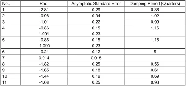
We investigate the local stability of the model, given the estimated parameters, using the linear approximation of the model around the equilibrium point. The estimated characteristic roots of the linearized model together with their asymptotic standard errors are presented in Table 1 below.

Table 1: Characteristic Roots of the Model

No.: Root Asymptotic Standard Error Damping Period (Quarters)

1 -2.81 0.29 0.36

2 -0.98 0.34 1.02

3 -1.01 0.22 0.99

4 -0.86

1.09*i

0.15 0.23

1.16

5 -0.86

-1.09*i

0.15 0.23

1.16

6 -0.21 0.12 5

7 0.014 0.015

8 -1.82 0.25 0.56

9 -1.65 0.18 0.61

10 -1.44 0.19 0.69

11 -1.08 0.25 0.93

All but one of the estimated characteristic roots of the continuous time model have negative real parts. The positive eigenvalue is insignificant and smallest in absolute value compared to the other characteristic roots, which allows us to use the model for practical purposes even though from a theoretical point of view the equilibrium path of the continuous model is not stable.

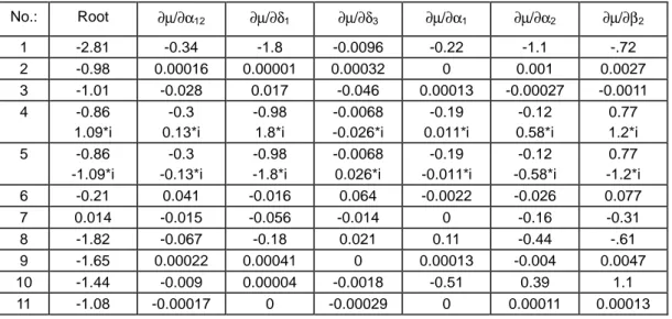
By sensitivity analysis, we mean the analysis of the effect of changes in the parameters on the characteristic roots of the model. The full size of the sensitivity matrix has a dimension of 33x11. We obtain the size of this matrix by multiplying the number of the estimated parameters (i.e. 33) by the number of the characteristic roots (i.e. 11). Table 2 below shows the partial derivatives of the characteristic roots with respect to the “policy parameters” (the parameters entering equation (17)) and some relatively large partial derivatives, since this implies that the particular parameter crucially effects the stability of the model.