Preparations for the Spin-Filtering Experiments at COSY/Jülich

Preparations for the Spin-Filtering Experiments at COSY/Jülich

Inaugural-Dissertation zur

Erlangung des Doktorgrades

der Mathematisch-Naturwissenschaftlichen Fakultät der Universität zu Köln

vorgelegt von

Christian Weidemann

aus Jena

Berichterstatter: Prof. Dr. H. Ströher Prof. Dr. J. Jolie

Tag der mündlichen Prüfung: 21.10.2011

ii

A ^BSTRACT

Polarized antiprotons allow unique access to a number of fundamental physics observables.

One example is the transversity distribution which is the last missing piece to complete the knowledge of the nucleon partonic structure at leading twist in the QCD-based parton model. The transversity is directly measurable via Drell-Yan production in double polarized antiproton-proton collisions. This and a multitude of other findings, which are accessible via ~ p~ p ¯ scattering experiments, led the Polarized Antiproton eXperiments (PAX) collaboration to propose such investigations at the High Energy Storage Ring (HESR) of the Facility for Antiproton and Ion Research (FAIR).

Already the production of intense polarized antiproton beams is still an unsolved problem.

The PAX anticipated time plan to experiments at HESR mainly consists of three phases.

PAX@COSY, as first step, is aiming for an optimization of the polarization build-up in proton beams at the Cooler Synchrotron COSY Jülich. The spin-filtering method, where the originally unpolarized beam becomes polarized due to the spin-dependent part of the hadronic interaction with a Polarized Internal Target (PIT), will be applied. The feasibility of this method was shown to work for protons by the Filter Experiment (FILTEX) at the Test Storage Ring (TSR) in Heidelberg. PAX@CERN will determine the spin-dependent cross sections in ~ p~ ¯ p scattering at beam energies of 50 − 450 MeV using the antiproton beam of the Antiproton Decelerator (AD) at CERN. PAX@FAIR constitutes the third phase where the antiproton beam will be polarized in a dedicated Antiproton Polarizer Ring (APR) at the HESR, converted into a double-polarized proton-antiproton collider, in order to study the transverse spin structure of nucleons.

The present thesis discusses the preparations for the spin-filtering experiments at COSY. This

includes the successful installation and commissioning of the experimental equipment such

as a low-β section, a dedicated pumping system, an Atomic Beam Source (ABS), a Breit-

Rabi Polarimeter (BRP), and a target chamber with an openable storage cell. In addition,

the accomplished investigations of the beam lifetime dependencies, resulting in significantly

improved beam lifetimes, and relevant machine parameters, e.g., the machine acceptance, are

described. The results are utilized to calculate the expected polarization build-up in a cooled

and stored proton beam with a kinetic energy of 49.3 MeV using a target with an areal density

of 5 · 10

atoms/cm

. Simulations of the determination of the beam polarization using elastic

proton-deuteron scattering and a polarimeter, that consists of silicon micro-strip detectors,

allows one to estimate the achievable precision of the measurement of the spin-dependent

total hadronic cross section. The presented results constitute the basis of a beam time request

for transverse spin-filtering to the COSY Program Advisory Committee (PAC), which was

approved in spring 2011.

Z USAMMENFASSUNG

Gespeicherte polarisierte Antiprotonen ermöglichen eine Vielzahl von bedeutenden Experi- menten im Bereich der Teilchenphysik. Hierzu gehört die direkte Messung der sogenannten Transversity, welche als letztes fehlendes Stück zur Beschreibung der partonischen Struktur des Nukleons im Rahmen der Quantenchromodynamik (QCD) angesehen wird. Mit Hilfe der Drell-Yan Produktion in doppeltpolarisierten Proton-Antiproton Streuexperimenten ist eine Untersuchung der transversalen Spinstruktur der Nukleonen möglich. Aufgrund dieser und einer Fülle weiterer möglicher wesentlicher Erkenntnisse wurden Untersuchungen dop- peltpolarisierter Antiproton-Proton Kollissionen am High Energy Storage Ring (HESR) der Facility for Antiproton and Ion Research (FAIR) von der Polarized Antiproton eXperiments Kollaboration (PAX) vorgeschlagen.

Hierbei ist bereits die Erzeugung intensiver polarisierter Protonenstrahlen eine anspruchsvol- le und bisher ungelöste Aufgabe. Der PAX Zeitplan hin zu Experimenten am HESR besteht im Wesentlichen aus drei Phasen. Im ersten Schritt wird PAX@COSY den Polarisationsaufbau mit Protonen am Cooler Synchrotron COSY in Jülich optimieren. Anwendung findet hierbei die Spinfilter Methode bei der ein anfangs unpolarisierte Strahl aufgrund der spinabhängigen hadronischen Wechselwirkung mit einem polarisierten Target polarisiert wird. Ein erfolgreicher Test dieser Methode wurde für Protonen bereits im Rahmen des Filter Experiments (FILTEX) am Test Storage Ring (TSR) in Heidelberg durchgeführt. PAX@CERN soll im zweiten Schritt mit dem Antiprotonenstrahl des Antiproton Decelerators (AD) am CERN zeigen, wie groß die spinabhängigen Wirkungsquerschnitte in der Proton-Antiproton Streuung sind. PAX@FAIR bildet die dritte Phase, in der die Antiprotonen in einem dedizierten Speicherring, dem Antiproton Polarizer Ring (APR), polarisiert werden. Mit Hilfe des polarisierten Antiprotonenstrahles soll in Streuexperimenten in einem doppelt- polarisierten Proton-Antiproton Collider die Vermessung der transversalen Spinstruktur des Protons erreicht werden.

Die vorliegende Arbeit erläutert die Vorbereitungen für das geplante Spinfilter Experiment

an COSY. Im Rahmen dieser Vorbereitungsphase wurde unter anderem das notwendige

experimentelle Equipment, bestehend aus einer sogenannten low-β Sektion, einem leis-

tungsfähigen Vakuumsystem, einer Atomstrahlquelle, einem Breit-Rabi Polarimeter und

einer Targetkammer mit auffahrbarer Speicherzelle, installiert und erfolgreich in Betrieb

genommen. Des Weiteren wurden Messungen zur Abhängigkeit der Strahllebensdauer

mit dem Resultat einer signifikanten Lebensdauererhöhung und detaillierte Studien zu

relevanten Maschinenparametern, wie z.B. Akzeptanzwinkel, durchgeführt. Die Ergebnisse

dieser Studien dienen als Grundlage zur Berechnung des erwarteten Polarisationsauf-

baus in einem gespeicherten, gekühlten Protonenstrahl bei einer kinetischen Energie von

49.3 MeV und einer Targetdichte von 5 · 10

Atome/cm

. Die weiterhin durchgeführten

Simulationsrechnungen zur Messung dieser Polarisation mit Hilfe von elastischer Proton-

Deuteron Streuung und eines Polarimeters, bestehend aus Siliziumstreifendetektoren, geben

Aufschluss über die benötigte Messzeit und die erreichbare Genauigkeit der Messung des

spinabhängigen totalen Wirkungsquerschnittes mit transversaler Strahlpolarisation. Auf der

Basis der präsentierten Ergebnisse wurde ein Experimentantrag der PAX Kollaboration an

das COSY Program Advisory Committee (PAC) eingereicht und vom PAC bewilligt.

C ^ONTENTS

1. Physics Case 1

1.1. Proton Structure . . . . 1

1.1.1. Elastic Electron-Nucleon Scattering . . . . 2

1.1.2. Deep Inelastic Scattering . . . . 3

1.1.3. Bjørken Scaling . . . . 5

1.1.4. Quark Parton Model . . . . 5

1.1.5. Spin Distribution of the Nucleon . . . . 7

1.2. Polarized Antiproton Experiments . . . . 7

1.2.1. Overview . . . . 7

1.2.2. Transversity Distribution . . . . 8

1.2.3. Production of Polarized Antiprotons . . . . 9

2. Spin Filtering in Storage Rings 11 2.1. Beam Dynamics in Storage Rings . . . . 11

2.1.1. Linear Beam Optics . . . . 11

2.1.2. Beam Loss Mechanisms . . . . 14

2.1.3. Beam Temperature and Beam Cooling . . . . 17

2.2. The Filter Experiment (FILTEX) - Proof of Principle . . . . 19

2.3. Theoretical Foundations of Spin Filtering . . . . 21

2.3.1. Polarization Build-up in a Stored Beam . . . . 21

2.3.2. Understanding the FILTEX Results . . . . 22

2.4. Beam Lifetime and Figure of Merit . . . . 23

3. Experimental Setup for the Spin-Filtering Experiments at COSY 27 3.1. COSY . . . . 27

3.1.1. COSY Lattice . . . . 28

3.1.2. COSY Vacuum System . . . . 29

3.1.3. Electron Cooler . . . . 30

3.1.4. Instrumentation . . . . 30

3.2. PAX Installation . . . . 33

3.2.1. PAX Vacuum System . . . . 34

3.2.2. PAX low-β Section . . . . 35

3.2.3. Atomic Beam Source (ABS) . . . . 36

3.2.4. Target Chamber and Openable Storage Cell . . . . 39

3.2.5. Holding Field System . . . . 40

3.2.6. Target Gas Analyzer and Breit-Rabi Polarimeter . . . . 42

3.3. ANKE as a Polarimeter . . . . 43

3.3.1. Deuterium Cluster Target . . . . 43

3.3.2. Silicon Tracking Telescopes (STTs) . . . . 43

4. Commissioning for Spin Filtering at COSY 47 4.1. Commissioning of the low-β Section . . . . 47

4.2. Working Point Adjustment . . . . 50

Contents

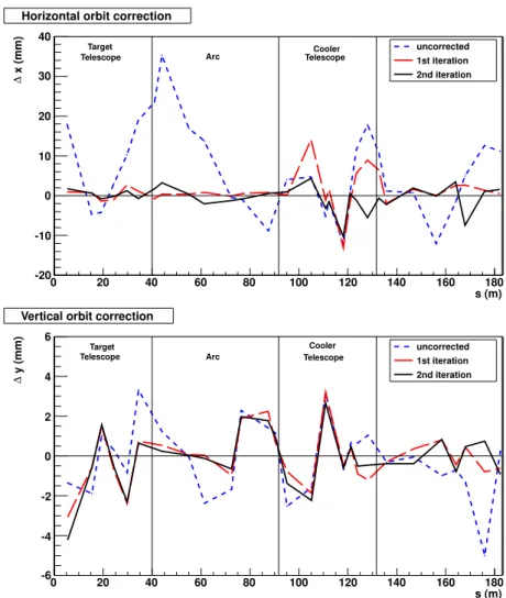
4.3. Closed-Orbit Correction Procedure . . . . 51

4.4. Single Intrabeam Scattering . . . . 52

4.5. Machine Acceptance and Beam Size . . . . 56

4.5.1. Kicker Measurement for Different Ion Optics . . . . 56

4.5.2. Acceptance Angle and Beam Position at the PAX Target Place . . . . 57

4.5.3. Measurement of the Beam Width at the Target Position . . . . 64

4.6. Target Related Issues . . . . 65

4.6.1. Holding Field Commissioning . . . . 66

4.6.2. Openable Storage Cell Commissioning and Target Density Measurement 68 4.6.3. Lifetime Contributions of the Polarized Target . . . . 70

4.7. How to Set Up the Beam for Spin-Filtering Experiments . . . . 73

5. Outline of the COSY Spin-Filtering Experiment 75 5.1. Polarization Build-up . . . . 76

5.2. Beam Polarization Measurement at ANKE . . . . 76

5.2.1. Setup for Polarization Measurement . . . . 77

5.2.2. Event Selection . . . . 80

5.2.3. Determination of the Beam Polarization . . . . 82

5.2.4. Systematic Errors . . . . 82

5.2.5. Results . . . . 85

6. Perspectives and Summary 87 6.1. Summary . . . . 88

6.2. Status and Outlook . . . . 89

6.3. Spin-Filtering Experiments at AD . . . . 90

A. Approximations for Intensity and Figure of Merit 95 A.1. Exact Calculations . . . . 96

A.2. Approximate Calculations . . . . 96

A.3. Comparison of Results . . . . 97

B. Determination of the Optimal Cycle 99 C. Holding Field System 101 D. Matrix Formalism and Measurement of the β Function 105 E. Estimation of the Target Density from the Cell Dimensions 109 F. PAX Sequencer 111 G. Summary of Experiment Simulations for the PAX Detector 113 G.1. Event Generation . . . 114

G.2. Event Detection . . . 115

G.3. Diagonal Scaling . . . 115

G.4. Results . . . 116

List of Figures 117

List of Tables 119

Bibliography 123

x

1. P ^HYSICS C ^ASE

The QCD

description of the partonic structure of the nucleon is in leading twist based on three structure functions, namely the well studied quark distribution q(x, Q

), the helicity distribution ∆q(x, Q

) and the largely unknown transversity distribution δq(x, Q

). A first direct measurement of this transversity distribution of the valence quarks in the proton has been proposed by the Polarized Antiproton eXperiments collaboration (PAX) at the High Energy Storage Ring (HESR) [1]. Since it is directly accessible uniquely via double polarized proton-antiproton scattering, polarized antiproton beams are a prerequisite to address this important topic. Therefore, in 2005 the PAX collaboration suggested to provide for the first time an intense polarized antiproton beam by the spin-filtering method, which is based on the spin-dependent part of the hadronic cross section.

The present description of the proton structure and how it was developed on the basis of scattering experiments is illustrated in Sec. 1.1. A detailed report on the planned experimental program of the PAX collaboration is given in Sec. 1.2.

1.1. Proton Structure

Since its very beginning, physics has pondered the question of what the fundamental building blocks of matter are. In the 19th century all matter was shown to be composed of atoms. After the discovery of the electron by Joseph John Thomson in 1897 [2], it was realized that there has to be a positively charged center within the atom to balance the negative electrons and create electrically neutral atoms. This center was found to be the atomic nucleus by Rutherford, Geiger and Mardsen [3, 4], whose alpha scattering experiments were the first experiments, in which individual particles were systematically scattered and detected.

Since the beginning of atomic physics nothing has improved the understanding of the inner structure of matter more than scattering experiments. They led to the discovery of the proton in 1919 by Rutherford [5] and almost 50 years later it became clear, that this particle possesses a substructure.

The enhancement of the performance of particle accelerators over the past decades, led to a dramatic increase of the projectile energies and thus their power to resolve structures at small distances. Inclusive Deep Inelastic Scattering (e + p → e

+ X) experiments at SLAC

, where a proton breaks up, allowed for the verification of the existence of point-like sub-nucleonic particles (partons) by Bjørken and Feynman [6–8]. These spin-

/

particles with fractional electric charge and a new degree of freedom called flavor, later identified as quarks, had been predicted earlier by Gell-Mann and Zweig [9, 10]. In the Quark Parton Model (QPM), which was developed at that time, two up quarks (u) with electrical charge +

/

e and one down quark (d) with -

/

e constitute one proton with a total charge of +e.

However, the discovery made in 1972 that roughly only 50 % of the nucleon momentum is carried by quarks [11] is in contradiction to this model. This discrepancy could be explained within the framework of QCD, the gauge theory of strong interactions. According to this

1

Quantum Chromodynamics

2

Stanford Linear Accelerator Center

1. Physics Case

theory, which requires the existence of color as an additional degree of freedom of the quarks, the missing momentum of the nucleon is carried by the gluons, the “massless“ vector gauge bosons mediating the strong force. The gluons can split into a virtual quark-antiquark pair (¯ qq), called sea quarks [12], which can annihilate back into gluons.

In the following, the present understanding of the proton structure by means of the QPM and how it developed with the help of elastic and deep inelastic lepton-nucleon scattering is illuminated. This points out the substantial physics potential of double polarized pp ¯ scattering experiments proposed by the PAX collaboration.

1.1.1. Elastic Electron-Nucleon Scattering

In elastic scattering of electrons off protons (e +p → e +p), which is assumed to be dominated by single-photon exchange (Fig. 1.1), the target proton stays intact and no new particles are created.

q γ

p P’

p

P

e k’

e

k

Fig. 1.1: Feynman diagram of elastic electron-proton scat- tering, here

and

are the four-momenta of the electron and proton before and after the collision, respectively, and

is the four-momentum of the virtual photon (the four-momentum transfer from the electron to the proton).

The elastic electron-proton scattering cross section, also known as Rosenbluth formula [13], can be written in the form

dσ dΩ =

dσ dΩ

Mott

·

G

+ τ G

1 + τ + 2τ G

tan

(Θ/2)

, (1.1)

where

dσ dΩ

Mott

= α

cos

(Θ/2)

4E

· sin

(Θ/2) · [1 + (2E

/M ) sin

(Θ/2)] (1.2) is the Mott cross section, that describes the elastic scattering of a relativistic spin-

/

particle off a spinless point-like particle. Here Θ is the electron scattering angle, M is the proton mass, E

is the incident electron energy, α =

/

is the electromagnetic coupling constant and τ =

/

with q = k − k

= P

− P the four-momentum of the exchanged virtual photon. k, k

and P, P

are the four-momenta of the electron and the proton before and after the collision, respectively. G

and G

are the electric and magnetic proton form factors, where the former is associated with the charge distribution and the latter with the magnetic moment distribution of the proton. The measurement of the cross section and the subsequent extraction of G

allows one to extract the root-mean-square charge radius r

of the proton [14]:

r

= Z

d

xr

ρ(r) = − 6 dG

(q

) dq

q₀²

= (0.81 ± 0.04 fm)

. (1.3) The same radius (0.8 fm) was also obtained for the magnetic distribution.

The extraction of G

and G

was achieved by the Rosenbluth separation method [13], which involves measuring cross sections at constant Q

(= − q

) and varying the beam energy and

2

1.1. Proton Structure

scattering angle to separate the electric and magnetic contributions. The extracted value for µG

/G

was shown to be Q

-independent (see Fig. 1 in [15]). Q

, the negative squared four momentum of the virtual photon Q

:= − q

= 4EE

sin

(Θ/2), is a measure of the spatial scale that can be resolved by a virtual photon with the wavelength λ =

/

, where v :=

= E − E

is the energy carried by the virtual photon. Since G

in Eq. (1.1) is multiplied by τ , the cross section becomes dominated by G

as Q

increases. Consequently, the extraction of G

is more difficult above Q

= 1 GeV.

Recent experiments at the Jefferson laboratory using polarization observables indicate an unexpected Q

-dependence of the ratio of the magnetic and electric form factors of the proton [15, 16]. Reasons for the discrepancy between the two methods have been indicated in two photon exchange [17, 18].

1.1.2. Deep Inelastic Scattering

In deep inelastic lepton-nucleon scattering (DIS), the nucleon N breaks up and forms a hadronic final state X, due to an increased lepton-beam energy and thus a larger momentum transfer:

l + N → l

+ X. (1.4)

Since leptons do not interact via the strong force, they are used as an electromagnetic probe to measure a variety of parton distribution functions and related observables. Figure 1.2 shows a sketch of the DIS process in the one-photon exchange approximation.

q γ

P

p P

e k’

e

k

Fig. 1.2: Feynman diagram of deep inelastic electron-proton scattering.

is the squared four-mo- mentum of the exchanged photon and

and

represent the target proton and the hadronic final

state four-momenta, respectively.

The kinematics can be characterized by Q

as described in Sec. 1.1.1, by the so-called Bjørken scaling variable x

=

which is the fraction of the proton momentum carried by the hard- scattered parton and by the squared invariant mass of the target-nucleon – virtual-photon system W

:= (P + q)

= M

+ 2M v − Q

. Combining the latter two variables allows one to determine the mass excitation (change of initial proton mass) caused by the scattering process

W

− M

= 2M v(1 − x). (1.5)

Therefore, the elastic limit corresponds to x → 1, with W

= M

, while x < 1 corresponds to the inelastic regime, in which W

> M

.

Averaging over all spins in the initial state of the scattering process and summing over the spins in the final state leads to the spin-independent part of the cross section [7, 19]

d

σ

dΩdE

=

dσ dΩ

Mott

2

M F

(x, Q

) tan

(Θ/2) + 1

v F

(x, Q

)

, (1.6)

1. Physics Case

where

Mott

is the Mott cross section, as described earlier. F

(x, Q

) := M W

(v, Q

) and F

(x, Q

) := vW

(v, Q

) are the spin-independent structure functions. The deviation from the Mott cross section denoted by the second term of Eq. (1.6) appears due to the composite nature of the proton.

The spin-dependent part of the cross section can be isolated by measuring the difference of the cross sections obtained with two opposite target spin states. In this case the unpolarized components cancel. If both the incident lepton beam and the target protons are longitudinally polarized one obtains [20, 21]

d

σ

dxdy − d

σ

dxdy = 4α

sxy

2 − y − γ

y

2

g

(x, Q

) − γ

yg

(x, Q

)

, (1.7)

where → indicates the spin orientation of the incoming electron and ⇐ , ⇒ the two different spin states of the target proton. Here s = (P + Q)

denotes the center of mass energy squared, y =

/

lab

=

/

is the fractional energy transfer from the lepton to the nucleon, γ = (2M x)/Q, and g

(x, Q

) and g

(x, Q

) are the polarized structure functions. Figure 1.3 displays the g

(x) world results for protons, neutrons and deuterons as a function of the Bjørken variable x.

In case of a transverse target polarization with respect to the incoming lepton direction, the polarized cross section becomes

d

σ

dxdydφ

− d

σ

dxdydφ

= 4α

sxy γ

r

1 − y − γ

y

4

γg

(x, Q

) + 2g

(x, Q

)

cos φ

, (1.8) where φ

is the azimuthal angle of the target spin vector S ~ with respect to the lepton beam direction.

-0.02 0 0.02 0.04 0.06 0.08

-0.02 0 0.02 0.04 x g1p

EMC E142 E143 SMC HERMES E154 E155 JLab E99-117 COMPASS CLAS

x g1d

x x g1n

-0.02 0 0.02

10^-4 10^-3 10^-2 10^-1 1

Fig. 1.3.: The spin-dependent structure function

of the proton, deuteron, and neutron (from

He target), measured in deep inelastic scattering of polarized electrons/positrons [20].

4

1.1. Proton Structure

1.1.3. Bjørken Scaling

The nucleon structure has been studied by deep inelastic scattering experiments performed at SLAC [22] and the results show, that the spin-independent structure functions F

and F

are approximately Q

-independent in the large momentum transfer region

F

(x, Q

) ≈ F

(x) (Q

M

), (1.9) as it was predicted by Bjørken [6]. He reasoned this behavior in the high-energy or Bjørken limit, defined by

lim

=

 



Q

→ ∞ v → ∞ , x fixed

(1.10)

in the case that the proton is composed of point-like constituents. F

shows the same Q

- independence, since F

and F

are related to each other by F

(x) = 2xF

(x) according to the Callan-Gross relation [23]. This phenomenon, known as Bjørken scaling or scale invariance is in contrast to the strong Q

-dependence of the elastic form factors, which stands for an inner structure of the proton, because it implies that the electromagnetic probe (lepton) measures the same proton structure, independent on the spatial resolution as it is the case for scattering from point-like constituents [7]. The Bjørken scaling and the conclusion from other experiments that these constituents are fermions [24], were the first dynamical evidences of the quarks.

With the larger accuracy of the next generation DIS experiments at FNAL

[25], at CERN

[26, 27], and at the HERA

electron-proton collider [28] in conjunction with the broadening of the kinematic regions a noticeable Q

-dependence appeared (see Fig. 1.4). F

increases with Q

for low x (x ≤ 0.003) and decreases for large x (x ≥ 0.6). The observed violation of the Bjørken scaling was interpreted within the framework of the QCD as the evidence of the dynamical structure of the proton.

As in detail discussed in [11], the sum of the momentum fractions of all the quarks (including antiquarks) can be determined via integration of F

(x). The extracted value of the momentum carried by quarks is only about 50% of the total momentum of the proton. Since the photon only probes the charged particles, this observation is consistent with about

/

of the nucleon momentum being carried by the exchange particles of the quark interaction, the gluons.

1.1.4. Quark Parton Model

In the QPM, developed by Feynman and Bjørken, the momentum and spin distribution of the quarks inside the proton are characterized at leading twist by three fundamental parton distribution functions (PDF): the quark distribution q(x, Q

), which is the probability of finding a quark with a fraction x of the longitudinal momentum of the parent hadron; the helicity distribution ∆q(x, Q

), which measures the net helicity of a quark in a longitudinally polarized hadron; and the transversity distribution δq(x, Q

) (more usually denoted as h

(x, Q

)), the net transverse polarization in a transversely polarized hadron [29, 30]. They

1

Fermi National Accelerator Laboratory

2

European Organization for Nuclear Research

3

Hadron Electron Ring Accelerator

1. Physics Case

Q² (GeV²) F2(x,Q2 ) * 2

i x

H1 ZEUS BCDMS E665 NMC SLAC

10^-3 10^-2 10^-1 1 10 10² 10³ 10⁴ 10⁵ 10⁶ 10⁷ 10⁸ 10⁹

10^-1 1 10 10² 10³ 10⁴ 10⁵ 10⁶

Fig. 1.4.: The proton structure function

measured in electromagnetic scattering of positrons on protons (collider experiments ZEUS and H1), in the kinematic domain of the HERA data, for

and for electrons (SLAC) and muons (BCDMS, E665, NMC) on a fixed target. The data are plotted as a function of

in bins of fixed

[20] .

are defined by

q

(x) = q

(x) + q

(x), (1.11)

∆q

(x) = q

(x) − q

(x), and (1.12) h

(x) = q

(x) − q

(x). (1.13) Here q

(x) and q

(x) are the probability densities to find a quark of flavor f with momentum fraction x and spin parallel or antiparallel to the spin of the longitudinally polarized proton. q

(x) and q

(x) are the probability densities to find a quark with its spin aligned or anti-aligned to the spin of a transversely polarized proton.

The spin-independent and spin-dependent structure functions, which can be measured in DIS, can now be interpreted within the QPM as the charge-weighted sums over the quark flavors (including anti-quarks) of the corresponding parton distribution functions (PDF)

F

(x) = 1 2

X

f

e

q

(x), (1.14)

g

(x) = 1 2

X

f

e

∆q

(x), (1.15)

where e

is the fractional charge carried by the quarks. Consequently, the first two of these PDFs are well known, whereas the transversity distribution, which describes the quark

6

1.2. Polarized Antiproton Experiments

transverse polarization inside a transversely polarized proton, is only little-known. Since it is directly measurable by Drell-Yan production q q ¯ → (γ, Z) → l

l

in double polarized p¯ p collisions [31], the PAX collaboration proposes a dedicated measurement with polarized antiproton beams [32] at the Facility for Antiproton and Ion Research (FAIR) [33], using the HESR upgraded to a Proton-Antiproton Collider.

1.1.5. Spin Distribution of the Nucleon

The proton is a fermion with spin

/

and, as a composite particle, the question arose how its spin originates from its constituents. 20 years ago, results from deep inelastic muon-proton scattering experiments performed by the European Muon Collaboration (EMC) suggested that the valence quarks intrinsic spin contributes only 25 − 30% to the proton spin [34, 35]

instead of 60% predicted by relativistic quark models. As an immediate consequence the question of the additional sources of the spin within the nucleon arises, which inspired a vast program of theoretical activities and new experiments [36]. One goal is the decomposition of the longitudinal spin components [37]

1 2 = 1

2 X

q

∆q + ∆g + L

+ L

, (1.16)

where ∆q and ∆g denote the longitudinal spin contribution of the quarks (helicity) and gluons, respectively, and L

and L

are the orbital angular momentum contributions. A significant part of the spin could be carried by gluons, sea quarks and orbital angular momenta of quarks and gluons. The contribution of the sea quark polarization is consistent with zero as it has been measured by the HERMES experiment at DESY [38, 39]. The solution of this problem, called “spin crisis”, was also not found by the COMPASS experiment at CERN or in polarized proton-proton collisions (PHENIX and STAR at RHIC), which determined a gluon polarization much to small to explain the 30% missing according to the theoretical predictions [40–42].

1.2. Polarized Antiproton Experiments

1.2.1. Overview

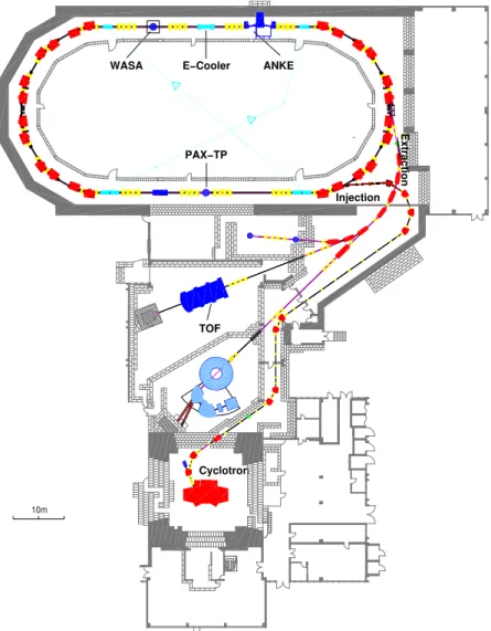
The HESR storage ring for antiprotons included in the FAIR project is to be build at GSI in Darmstadt/Germany. The machine is planned to provide high luminosity antiproton beams in the momentum range from 1.5 GeV/c < p < 15 GeV/c (831 MeV < T < 14.1 GeV) [1]. In order to study double polarized p p ¯ collisions proposed by the PAX collaboration, it would need to be upgraded into a collider. This consists of an Antiproton Polarizer Ring (APR) to polarize antiprotons at energies of 50 − 500 MeV and a Cooler Synchrotron Ring (CSR) to store protons or antiprotons at energies up to 3.5 GeV. As depicted in Fig. 1.5, the polarized antiprotons circulate in the CSR whereas the polarized protons circulate in the HESR.

Polarized antiprotons, produced by spin filtering with an internal polarized gas target, where

the beam becomes polarized because of a larger selective removal of one spin state compared

to the other (see also Section 2.3), allow a unique access to a number of new fundamental

physics observables. This includes a first measurement of the transversity distribution of the

valence quarks in the proton, a direct determination of the transverse double spin asymmetry

in the p¯ p total cross section, and a first measurement of the moduli and the relative phase of

the time-like electric and magnetic form factors G

of the proton [1]. The measurement of

the transversity is explained in detail in the following.

1. Physics Case

Fig. 1.5.: Proposed HESR upgrade for FAIR. The antiprotons are polarized in the APR by spin filtering. At the PAX interaction point polarized antiprotons from the CSR will collide with polarized protons from the HESR.

1.2.2. Transversity Distribution

The transversity distribution h

(x) is the last missing piece leading-twist of the QCD description of the partonic structure of the nucleon. Unlike the more conventional unpolarized quark distribution q(x) and the helicity distribution ∆q(x), the transversity h

(x) can neither be accessed in deep inelastic scattering of leptons off nucleons, due to its chiral- odd nature, nor can it be reconstructed from the knowledge of q(x) and ∆q(x) [43–46]. Since electroweak and strong interactions conserve chirality, h

(x) cannot occur alone, but has to be coupled to a second chiral-odd quantity. This is possible in polarized Drell-Yan processes, where one measures the product of two transversity distributions, and in Semi-Inclusive Deep Inelastic Scattering (SIDIS), where one couples h

(x) to a new unknown fragmentation function, the Collins function [47]. Similarly, one could couple h

(x) and the Collins function in transverse single-spin asymmetries (SSA) in inclusive processes like p

p → πX [1].

The HERMES experiment at DESY

was the first to measure a nonzero, Collins asymmetry [48, 49], which would allow one to extract the transversity once the Collins function is known.

A first extraction of h

(x), based on a global fit of the data from HERMES, COMPASS [50]

and BELLE [51, 52] has been reported in [53]. Since the extraction of the transversity uses the projection of the Collins asymmetries measured at BELLE at Q

= 110 GeV

to HERMES energies ( h Q

i = 2.4 GeV

), the theoretical uncertainties are rather large.

The most direct way to obtain information on transversity is the measurement of the double transverse spin asymmetry A

in Drell-Yan processes (Fig. 1.6) with both transversely polarized protons and antiprotons

A

= dσ

− dσ

dσ ↑↑ + dσ

= ˆ a

P

q

e

h

(x

, Q

)h

(x

, Q

) P

q

e

q(x

, Q

)¯ q(x

, Q

) , (1.17) where q = u, d, ... and q ¯ = ¯ u, d, ..., ¯ Q is the lepton pair invariant mass and x

are the fractional longitudinal momenta of the colliding hadrons, which are carried by the annihilating quark and antiquark. The double spin asymmetry a ˆ

of the QED process

1

Deutsches Elektronen-Synchrotron

8

1.2. Polarized Antiproton Experiments

q p >

X

¯ >

p X

¯ q

γ Q

l

l

Fig. 1.6: Feynman diagram of the Drell-Yan process

.

q q ¯ → l

l

is given by

ˆ

a

= sin

Θ

1 + cos

Θ cos 2φ, (1.18)

where Θ is the polar angle of the lepton in the l

l

rest frame and φ is the azimuthal angle with respect to the proton polarization.

The asymmetry A

in Drell-Yan processes with transversely polarized protons is at present exclusively measurable at the Relativistic Heavy Ion Collider (RHIC). There, the product of two transversity distributions is measured, one for a quark (h

) and one for an antiquark (h

)(both in a proton). Since they are assumed to be equivalent one basically determines (h

)

. At RHIC energies measurements at τ = x

x

= Q

/s ' 10

are expected, which mainly leads to the exploration of the sea quark content of the proton, where the asymmetry A

is likely to be tiny. Moreover, the QCD evolution of transversity is such that, in the kinematical regions of RHIC data, h

(x) is much smaller than the corresponding values of

∆q(x, Q

) and q(x, Q

). All this makes the double spin asymmetry A

expected at RHIC very small, of the order of a few percents or less [1, 54, 55].

The golden channel to perform a self-sufficient measurement of A

is p ¯

p

→ l ¯ lX as proposed by the PAX collaboration. For typical PAX kinematics in the fixed target mode (s = 30 or 45 GeV

) one has τ = x

x

= Q

/s ' 0.2 − 0.3, which implies that only quarks (from the proton) and antiquarks (from the antiproton) with large x contribute, i.e., valence quarks for which h

(x) is expected to be large. A

/ˆ a

is expected to be as large as 30%.

When combining the fixed target and the collider operational modes (s ' 30 − 200 GeV

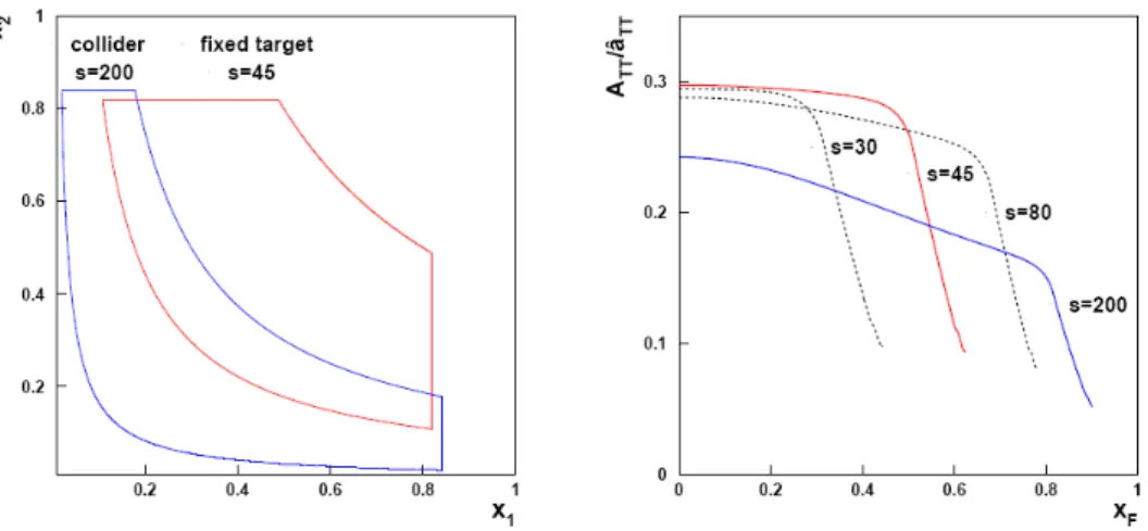
), the experiment will explore the kinematic regions as shown in the left panel of Fig. 1.7. In the right panel the expected A

/ˆ a

as a function of Feynman x

= x

− x

for Q

= 16 GeV

is shown.

While the direct access to transversity is the outstanding, unique possibility offered by the PAX proposal concerning the proton spin structure, there are several other spin observables related to partonic correlation functions. The measurements with a polarized antiproton beam can also provide completely new insights into the understanding of (transverse) single- spin asymmetries or the origin of the unexpected Q

-dependence of the ratio of the magnetic and electric form factors of the proton, which was illuminated in Sec. 1.1.2.

1.2.3. Production of Polarized Antiprotons

As shown above, polarized antiprotons will provide access to a wealth of single- and

double-spin observables. Therefore, the first major goal on the agenda of PAX is to provide

polarized antiprotons. Different suggestions, made at workshops in Bodega Bay 1985 [56] and

1. Physics Case

Fig. 1.7.: Kinematic region covered by the

measurement at PAX. In the asymmetric collider scenario (blue) antiprotons of

impinge on protons of

at c.m. energies of

and

. The fixed target case (red) represents antiprotons of

colliding with a fixed polarized target (

s ≈√

45 GeV). Right: The expected asymmetry as a function of Feynman xF

for different values of

[1].

Daresbury 2007 [57], like spin splitting in Stern-Gerlach separation [58] or the production of polarized antiprotons from the decay in flight of Λ ¯ hyperons [59] have not yet been tested or do not allow for efficient accumulation in a storage ring. The production of high luminosity polarized antiproton beams as a crucial prerequisite will be tested in spin-filtering studies at COSY/Jülich [60] and at AD/CERN [61]. The COSY accelerator will be utilized to test and commission the experimental equipment and repeat a spin-filtering experiment with protons in order to confirm our understanding of spin filtering in terms of the machine parameters.

Since PAX proposes to build a dedicated Antiproton Polarizer Ring (APR), obtaining a comprehensive knowledge about the experimental boundary conditions is crucial.

Afterwards, a first feasibility test of spin filtering with antiprotons and a measurement of the spin-dependent cross sections σ

and σ

(see Sec. 2.3.1) in the range from 50 to 450 MeV is planned to be carried out at the Antiproton Decelerator (AD) at CERN. This data will allow for the definition of the optimum working parameters of the APR.

10

2. S PIN F ILTERING IN S TORAGE

R INGS

Particle beams provided by accelerators are used in scattering experiments to study the structure and interaction of matter. The focus of current investigations, e.g., extraction of the transversity distribution from Drell-Yan production, requires the use of spin-polarized antiprotons. The spin-filtering method is proposed to pave the way toward such stored polarized antiproton beams.

The idea of spin filtering was first proposed by Csonka [62] in 1968 and can be described as a spin-selective attenuation of the particles circulating in a storage ring. An originally unpolarized beam becomes increasingly polarized by repeated interaction with a nuclear polarized internal gas target. A first feasibility test of polarizing beams of strongly interacting charged particles by spin filtering was carried out with protons at the Test Storage Ring (TSR) at MPIK

Heidelberg [63]. The Filter Experiment (FILTEX) from 1992 is described in more detail in Sec. 2.2. The theoretical interpretations, presented in Sec. 2.3, show that the small effective polarizing cross section demands for long filtering times. Consequently, particle beam dynamics and beam loss mechanisms have to be understood properly in order to optimize spin-filtering experiments. These aspects and how beam losses can be minimized by phase-space cooling are described in Sec. 2.1 in order to define the equipment and prerequisites for a spin-filter experiment.

2.1. Beam Dynamics in Storage Rings

One essential ingredient of particle accelerator experiments is the characterization of the particle beam in view of the particle motion and the interactions of the beam particles with each other and with internal targets. For the spin-filtering experiments as well as for the planned polarized antiproton experiments at AD, reasonably high luminosities of the polarized beams are crucial, which makes it indispensable to understand the beam loss mechanisms and how to minimize them.

2.1.1. Linear Beam Optics

The equations of particle motion in a closed orbit can be deduced by the second derivative of the position vector ~r

(s) =

, where F ~ = q(~v × B) ~ is the Lorentz force. For a particle moving in s-direction ~v = (0, 0, v

) (see Fig. 2.1) and considering only transverse magnetic fields B ~ = (B

, B

, 0) the betatron oscillations, that characterize the transverse displacement of the orbit with respect to the reference orbit, can be described by the linear equations of motion [64, 65]

1

Max-Planck-Institut für Kernphysik

2. Spin Filtering in Storage Rings

orbit

y s

x

ρ Θ

Fig. 2.1: Comoving right-handed coordinate system (s,

movement in accelerators, where

points in direction of motion.

is the angle of rotation and

the orbit curvature.

x

(s) + 1

ρ

(s) − k

(s)

x(s) = 1 ρ(s)

∆p

p , (2.1) y

(s) + k

(s)y(s) = 0. (2.2)

Here k

(s) =

and k

(s) =

are the normalized horizontal and vertical focussing strengths induced by a magnetic quadrupole field.

=

B

is the inverse bending radius due to a vertical magnetic dipole field. These functions are periodical and recur in each turn.

For

= 0 and

= 0, the general solution of Eq. (2.1) and (2.2) for z ∈ { x, y } is z(s) = p

β

(s) cos(ψ

(s) + ψ

) with ψ

(s) = Z

0

d˜ s

β

(˜ s) + ψ

(2.3) being the phase advance of the oscillation, β

(s) the betatron function, and

the beam emittance. Hence the position dependent amplitude of the betatron oscillation of a particle is described by E

(s) = p

β

(s) with the envelope E

(s). The betatron phase change per revolution ∆ψ

= ψ(s + C) − ψ(s) (C is the ring circumference) is of prime importance for the understanding of resonances. The betatron tune or working point, that illustrates the number of oscillation per turn is given by

Q := ∆ψ 2π = 1

2π I d˜ s

β(˜ s) . (2.4)

The beam lifetime strongly depends on the chosen betatron tunes. Because of the symmetry in a synchrotron like COSY, the magnetic structure after each full turn merges into itself (see Sec. 3.1.1). Consequently, the forces on the beam recur periodically. Therefore the tunes should be irrational numbers, while in practice one tries to stay far from the betatron resonances. The resonance condition is given by

mQ

= nQ

= l m, n, l ∈ N. (2.5)

Combining Eq. (2.3), z

(s) = −

√

p β(s) [α(s) cos(ψ(s) + ψ

) + sin(ψ(s) + ψ

)] , (2.6)

12

2.1. Beam Dynamics in Storage Rings

and γ(s) :=

, where α(s) := −

, allows for a description of the particle motion in the z − z

-plane, which is better known as transverse phase space. α, β and γ are also known as Twiss parameters. Here, the trajectory of a particle follows an ellipse described by

γ(s)z

(s) + 2α(s)z(s)z

(s) + β(s)z

(s) = , (2.7) which encloses a phase space equal to F = π

, as depicted in Fig. 2.2. Position and shape of the ellipse change along the orbit due to different Twiss parameters, but the area for a conservative system is invariant according to the Liouville’s theorem [67].

Z Z’

F=πZ

ϕ

−α_z^q_γ^Z

√ZγZ Z

√ZβZ

−αz qZ

βZ

qZ γZ qZ

βZ

tan 2ϕ=_γ−β^2α

Fig. 2.2: Phase space ellipse of the particle motion in the

-plane. The area enclosed by the ellipse is equal to

and

are the Twiss functions. The maximum amplitude of the betatron motion is

β, and the

maximum divergence (angle) of the betatron motion is

γ

[66].

For a determination of the emittance of a beam, which is an ensemble of particles with each particle having its own phase space ellipse, a Gaussian charge distribution is assumed

ρ(x, y) = N e

2πσ

σ

· exp

− x

2σ

− y

2σ

. (2.8)

ρ(x, y) characterizes the transverse charge distribution, with the standard deviations σ

and σ

. All particles with a distance of one standard deviation to the beam axis have an emittance of

= σ

(s)

β(s) , (2.9)

which is defined as the emittance of the beam. The emittance of the particle with the maximum possible phase ellipse equals the transverse acceptance of the accelerator (without closed-orbit deviation). It is given as

A = d

β

min

, (2.10)

where d is the free aperture at the location in the ring where A is minimal. Especially in storage rings a large A/ is crucial to minimize significant beam losses. The acceptance angle

∗

Here

mm mrad to

imply that the emittance as well as the acceptance is related to the area of a phase space ellipse [66].

2. Spin Filtering in Storage Rings

Θ

is defined as the maximum allowed angle kick, below which a scattered particle remains in the ring. For decoupled betatron oscillations in both planes it can be determined by [68]

1

Θ

= 1

2Θ

+ 1

2Θ

with 1

Θ

= β

A

. (2.11)

In case of a not vanishing momentum dispersion (

6 = 0) of the beam particles the beam orbit is manipulated by magnetic dipole components (

6 = 0). For a homogeneous magnetic field without gradients (k

= 0), Eq. (2.1) becomes

x

+ 1

ρ

· x = 1 ρ

∆p

p . (2.12)

Defining a dispersion orbit as

D

(s) + 1

ρ

D(s) = 1

ρ (2.13)

with

= 1 and solving the inhomogeneous differential equation, a total displacement from the reference orbit can be calculated

x(s)

= x(s) + x

(s) = x(s) + D(s) ∆p

p . (2.14)

A single particle in the beam is not longer moving along the ideal orbit, but oscillates around a dispersion orbit [67]. Thus the path length and the orbit frequency depend on the particle momentum. Since this plays an important role for longitudinal phase focussing the ratio of

∆L/L to ∆p/p is defined as momentum compaction factor α = ∆L/L

∆p/p . (2.15)

The preparation of a closed orbit with minimal distortions is a prerequisite for large beam lifetimes, which are essential for spin-filtering experiments. This includes the choice of a convenient betatron tune in order to prevent betatron resonances and to minimize the dispersion and the betatron function especially at positions with small free aperture.

2.1.2. Beam Loss Mechanisms

Since the polarization build-up rates in spin filtering are rather small, there is a need for long storage times in order to produce intense, polarized proton or antiproton beams with reasonable polarization. Therefore, the dominating particle loss mechanisms have to be understood and minimized. Once the ion beam is injected and circulating in the storage ring, coasting beam condition, various mechanisms give rise to particle losses. In general these are

• Betatron resonances.

• Beam target and/or residual gas Coulomb interactions comprising:

– energy loss, causing particle losses at the longitudinal acceptance

– emittance growth due to multiple small-angle scattering, causing losses at the transverse acceptance

– immediate loss of ions in a single collision where the scattering angle is larger than the transverse acceptance angle.

14

2.1. Beam Dynamics in Storage Rings

Energy loss and emittance growth can to a large extent be compensated by electron cooling, the technique applied at COSY for beam cooling at the lower beam energies (T

≤ 70 MeV).

• Single intrabeam scattering which is a Coulomb interaction between the beam particles causing emittance growth and possibly large momentum changes (Touschek effect).

• Beam losses due to recombination of beam particles with electrons from the electron cooler are known to be negligible. However, the production of neutral hydrogen atoms (H

) is large enough to be used as performance monitor [69] (Sec. 3.1.4).

• Hadronic interactions also lead to an immediate particle loss, but this is the effect to be exploited for the polarization build-up.

Betatron resonances

The resonance condition is given in Eq. (2.5). This means that the number of betatron oscillations per turn should be irrational numbers in order to avoid losses of beam particles.

Thus, the choice of a suitable working point is mandatory to achieve large beam lifetimes.

This procedure is in detail described in Sec. 4.2 (Fig. 4.4).

Energy loss

A charged particle that passes through matter looses energy in proportion to the density of a target through electromagnetic processes. The energy loss per single traversal δT and the knowledge of the stopping power (dE/dx) and the mass of the target atom m allow one to determine the effective target density d

,

d

= δT

(dE/dx)m . (2.16)

In storage rings the energy loss builds up in time due to a large number of circulations and causes a shift in the frequency of revolution f . Therefore the frequency shift in time is a measure of the target density or alternatively of the residual gas contributions [70],

d

=

1 + γ γ

1 η

1 (dE/dx)m

T

f

df

dt . (2.17)

Here γ is the Lorentz factor, and η is the frequency slip parameter defined as η =

− α. When the shift in frequency and respectively in momentum exceeds the longitudinal acceptance δ =

of the accelerator, the particle gets lost,

∆f f

1 η = ∆p

p

> δ. (2.18)

The energy loss caused by the polarized gas target, which will be used in spin-filtering experiments, can be balanced by electron cooling. Switching off the electron beam provides a reliable method to determine the target thickness from the observed frequency shift.

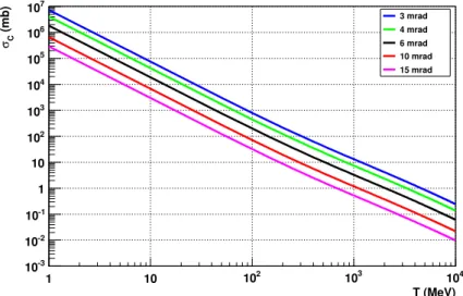
Single Coulomb scattering

The Coulomb-loss cross section can be derived by integration of the differential Rutherford cross section, for scattering angles larger than Θ

[71],

∆σ

= Z

0

Z

Θacc

dσ

dΩ dφ sin ΘdΘ = 4π Z

Z

r

β

γ

Θ

. (2.19)

Z

, Z

are the atomic numbers of the target (or residual gas) and the ion beam, respectively,

and r

= r

m

/m

is the classical ion radius. Θ

is assumed to be small. Consequently,

losses due to the residual gas are amplified in regions of small acceptance angles and large

2. Spin Filtering in Storage Rings

T (MeV)

1 10 10² 10³ 10⁴

(mb)Cσ

10-3

10-2

10-1

1 10 102

103

104

105

106

107

3 mrad 4 mrad 6 mrad 10 mrad 15 mrad

Fig. 2.3.: Coulomb cross section

as a function of the kinetic energy

for different acceptance angles

.

betatron functions. Inserting estimated parameters at COSY (Θ

≈ 6 mrad, T = 49.3 MeV) into Eq. (2.19) yields ∆σ

≈ 800 mb (Fig. 2.3). The lifetime due to single Coulomb scattering is given by

τ

= 1

∆σ

d

f , (2.20)

where d

is the target areal density and f the revolution frequency.

Touschek effect

Intense ion beams with small emittance as they are created by beam cooling reveal also phenomena of the mutual Coulomb interaction of the individual beam particles, called intrabeam scattering (IBS). Especially at low beam energies, IBS is a further mechanism leading to emittance growth. Large angle intrabeam scattering events known as Touschek effect may change the momentum of a single particle so that it is immediately lost at the longitudinal acceptance of the ring. The Touschek lifetime is given by [72, 73]

τ

= 4γ

β

· h √

β

i · C ·

· δ

√ π · I · c · r

, (2.21)

where

is the transverse rms beam emittance, I the number of circulating particles, C the ring circumference, β

the average betatron amplitude in the ring, r

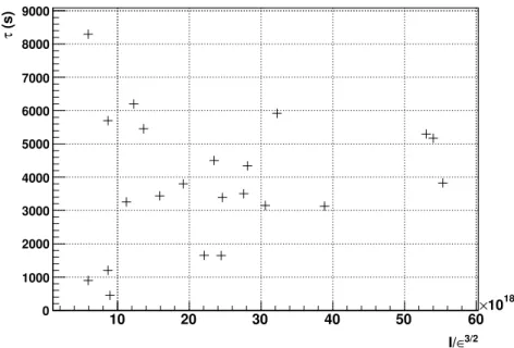
the classical particle radius, and δ the longitudinal machine acceptance as defined earlier. If single intrabeam scattering dominates the lifetime in the machine, one has to observe the corresponding dependencies on beam intensity, the beam emittance and momentum acceptance δ. The Touschek effect is an important beam loss factor in electron rings. How far it could be relevant for a proton machine is a topic of the machine studies in this work (see Sec. 4.4).

Hadronic interaction

The total hadronic cross section for pp collisions is shown in Fig. 2.4. For T = 49.3 MeV or p = 308 MeV/c, where the spin-filtering experiment at COSY is planned, the total hadronic cross section amounts to σ

≈ 50 mb. The lifetime due to hadronic interactions is given by

τ

= 1

σ

d

f . (2.22)

16

2.1. Beam Dynamics in Storage Rings

Fig. 2.4.: Hadronic cross section for

collisions as a function of laboratory beam momentum [20].

2.1.3. Beam Temperature and Beam Cooling

The terms temperature and cooling of a particle beam have been deduced from the kinetic gas theory. The beam temperature k

T is defined by the mean kinetic energy of the particle beam in the reference system that moves with the mean particle velocity. It is

3

2

k

T =

m h v

i , where k

is the Boltzmann constant. Therewith the transverse and longitudinal beam temperatures become k

T

=

h p

i ≈

mc

(γβ)

x

βx

+

y

and

1

2

k

T

=

h p

i ≈

mc

β

p

p

, respectively [65].

Scattering processes like those described in Sec. 2.4 cause a beam to change its phase space distribution. Multiple scattering, for example blows up the beam and increases the beam temperature, due to the growth of emittance and momentum distribution. Since those effects lead to intensity losses with time, one has to compensate the “beam heating“ by the help of dissipative forces. Thus, different techniques for beam cooling can be applied. At COSY phase-space cooling up to 600 MeV/c proton-beam momentum is achieved by electron cooling [69] and at larger momenta stochastic cooling is used [74, 75]. In the following electron cooling is described, since this technique is most useful and applicable at spin- filtering energies.

Electron cooling

Electron cooling as “an effective method of damping particle oscillations in proton and anti- proton storage rings” was first proposed by G. I. Budker in 1967 [76], and is an essential tool for many of todays accelerator experiments such as spin-filtering experiments. A first feasibility test of this technique, which shrinks the size, divergence and energy spread of a beam without removing particles, was performed in 1974 [77]. Since the phase space occupied by the stored particles is compressed, it is equivalent to reducing the temperature of the beam [71]. It is achieved by combining a circulating beam with a nearly monochromatic and parallel electron beam over a certain distance, where the “heat” is transfered from the ions to the electrons by Coulomb interaction. The electron beam is renewed and the velocity spread of the ion beam is reduced in all three coordinates.

A “cold”, dense electron beam is produced from a thermionic cathode and accelerated

electrostatically to the average velocity of the particles in the circulating beam. Guided by

the magnetic field of solenoids and toroids the electron beam is directed into the cooling

solenoid over a certain length. The dynamics of the cooling process in the interaction region