LECTURES ON TROPICAL METEOROLOGY

(1)

LECTURES ON TROPICAL METEOROLOGY

Roger K. Smith

April 13, 2015

(2)

Chapter 1 INTRODUCTION TO THE TROPICS

In geographical terminology “the tropics” refers to the region of the earth bounded by the Tropic of Cancer (lat. 23.5^◦N) and the Tropic of Capricorn (lat. 23.5^◦S). These are latitudes where the sun reaches the zenith just once at the summer solstice. An alternative definition would be to choose the region 30^◦S to 30^◦N, thereby dividing the earths surface into equal halves. Defined in this way the tropics would be the source of all the angular momentum of the atmosphere and most of the heat. But is this meteorologically sound? Some parts of the globe experience “tropical weather”

for a part of the year only - southern Florida would be a good example. While Tokyo (36^◦N) frequently experiences tropical cyclones, called “typhoons” in the Northwest Pacific region, Sydney (34^◦S) never does.

Riehl (1979) chooses to define the meteorological “tropics” as those parts of the world where atmospheric processes differ significantly from those in higher latitudes.

With this definition, the dividing line between the ”tropics” and the “extratropics” is roughly the dividing line between the easterly and westerly wind regimes. Of course, this line varies with longitude and it fluctuates with the season. Moreover, in reality, no part of the atmosphere exists in isolation and interactions between the tropics and extratropics are important.

Figure 1.1 shows a map of the principal land and ocean areas within 40^◦ latitude of the equator. The markedly non-uniform distribution of land and ocean areas in this region may be expected to have a large influence on the meteorology of the tropics. Between the Western Pacific Ocean and the Indian Ocean, the tropical land area is composed of multitude of islands of various sizes. This region, to the north of Australia, is sometimes referred to as the “Maritime Continent”, a term that was introduced by Ramage (1968). Sea surface temperatures there are particularly warm providing an ample moisture supply for deep convection. Indeed, deep convective clouds are such a dominant feature of the Indonesian Region that the area has been called “the boiler-box” of the atmosphere. The Indian Ocean and West Pacific region with the maritime continent delineated is shown in Fig. 1.2.

4

(5)

CHAPTER 1. INTRODUCTION TO THE TROPICS 5

Figure 1.1: Principal land and ocean areas between 40^◦N and 40^◦S. The solid line shows the 18^◦C sea level isotherm for the coolest month; the dot-dash line is where the mean annual range equals the mean daily range of temperature. The shaded areas show tropical highlands over 1000 m. (From Nieuwolt, 1977)

Figure 1.2: Indian Ocean and Western Pacific Region showing the location of the Maritime Continent (the region surrounded by a dashed closed curve).

(6)

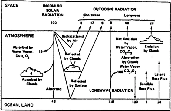
Figure 1.3: Zonally averaged components of the absorbed solar flux and emitted thermal infrared flux at the top of the atmosphere. + and −denote energy gain and loss, respectively. (From Vonder Haar and Suomi, 1971, with modifications)

1.1 The zonal mean circulation

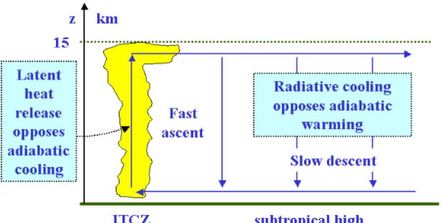
Figure 1.3 shows the distribution of mean incoming and outgoing radiation at the edge of the atmosphere averaged zonally and over a year. If the earth-atmosphere system is in thermal equilibrium, these two streams of energy must balance. It is evident that there is a surplus of radiative energy in the tropics and a net deficit in middle and in high latitudes, requiring on average a poleward transport of energy by the atmospheric circulation. Despite the surplus of radiative energy in the tropics, the tropical atmosphere is a region of net radiative cooling (Newell et al., 1974). The fact is that this surplus energy heats the ocean and land surfaces and evaporates moisture. In turn, some of this heat finds its way into the atmosphere in the form of sensible and latent heat and it is energy of this type that is transported polewards by the atmospheric circulation.

Figure 1.4 shows the zonally-averaged distribution of mean annual precipitation as function of latitude. Note that the precipitation is higher in the tropics than in the extratropics with a maximum a few degrees north of the equator. When precipitation occurs, i.e. a net amount of condensation without re-evaporation, then latent heat is released. The implication is that latent heat release may be an important effect in the tropics.

Figure 1.4 shows the zonally-averaged distribution of mean annual precipitation as function of latitude. Note that the precipitation is higher in the tropics than in the extratropics with a maximum a few degrees north of the equator. When precipitation occurs, i.e. a net amount of condensation without re-evaporation, then latent heat is released. The implication is that latent heat release may be an important effect

(7)

Figure 1.4: Mean annual precipitation as a function of latitude. (After Sellers, 1965) in the tropics.

A variety of diagrams have been published depicting the mean meridional circulation of the atmosphere (see. e.g. Smith, 1993, Ch. 2). While these differ in detail, especially in the upper troposphere subtropics, they all show a pronounced Hadley cell with convergence towards the equator in the low-level trade winds, rising motion at or near the equator in the so-called equatorial trough, which is co-located with the intertropical convergence zone (ITCZ), poleward flow in the upper troposphere and subsidence into the subtropical high pressure zones. The ITCZ is a narrow zone paralleling the equator, but lying at some distance from it, in which air from one hemisphere converges towards air from the other to produce cloud and precipitation.

It is characterized by low pressure and cyclonic relative vorticity in the lower troposphere. Usually the ITCZ is well marked only at a small range of longitudes at any one time. Figure 1.7 shows a case of an ITCZ marked by a very narrow line of deep convection across the Atlantic ocean, a little north of the Equator, while Fig. 1.8 shows an unusual case with the ITCZ stretching across much of the Pacific Ocean.

Figure 1.9 shows the zonally-averaged zonal wind component at 750 mb and 250 mb during June, July and August (JJA) and December, January and February (DJF). The most important features are the separation of the equatorial easterlies and middle-latitude westerlies and the variation of the structure between seasons.

In particular, the westerly jets are stronger and further equatorward in the winter hemisphere. The rather irregular distribution of land and sea areas in and adjacent to the tropics gives rise to significant variation of the flow with longitude so that zonal averages of various quantities may obscure a good deal of the action!

(8)

Figure 1.5: The mean annual meridional transfer of water vapour in the atmosphere (in 10¹⁵ kg). (After Sellers, 1965)

Figure 1.6: The mean meridional circulation and main surface wind regimes. (From Defant, 1958)

(9)

Figure 1.7: Visible satellite imagery from the EUMETSAT geostationary satellite at 0600 GMT on 19 May 2000 showing a well-formed ITCZ across the Atlantic Ocean.

Figure 1.8: Visible satellite imagery from the two geostationary satellites at 2100 GMT on 14 May 2003 showing a well-formed ITCZ across the entire Pacific Ocean.

1.2 Data network in the Tropics

One factor that has hampered the development of tropical meteorology is the relatively coarse data network, especially the upper air network, compared with the network available in the extra-tropics, at least in the Northern Hemisphere. This

(10)

Figure 1.9: Mean seasonal zonally averaged wind at 250 mb and 750 mb for (a) the equinox, (b) JJA, and (c) DJF as a function of latitude. The dashed line indicates the tropospheric vertical average. Units are m s⁻¹. (Adapted from Webster, 1987b) situation is a consequence of the land distribution and hence the regions of human settlement.

The main operational instruments that provide detailed and reliable information on the vertical structure of the atmosphere are radiosondes and rawinsondes. Fig-

(11)

CHAPTER 1. INTRODUCTION TO THE TROPICS 11 ure 1.10 shows the distribution and reception rates of radiosonde reports that were received by the European Centre for Medium Range Weather Forecasts (ECMWF) during April 1984. The northern hemisphere continents are well covered and reception rates from these stations are generally good. However, coverage within the tropics, with certain notable exceptions, is minimal and reception rates of many tropical stations is low. Central America, the Caribbean, India and Australia are relatively well-covered, with radiosonde soundings at least once a day and wind soundings four times a day. However, most of Africa, South America and virtually all of the oceanic areas are very thinly covered. The situation at the beginning of the 21st century is much the same.

Satellites have played an important role in alleviating the lack of conventional data, but only to a degree. For example, they provide valuable information on the location of tropical convective systems and storms and can be used to obtain

“cloud-drift” winds. The latter are obtained by calculating the motion of small cloud elements between successive satellite pictures. A source of inaccuracy lies in the problem of ascribing a height to the chosen cloud elements. Using infra-red imagery one can determine at least the cloud top temperature which can be used to infer the broad height range. Generally use is made of low level clouds, the motion of which is often ascribed to the 850 mb level (approximately 1.5 km), and high level cirrus clouds, their motion being ascribed to the 200 mb level (approximately 12 km). Clouds with tops in the middle troposphere are avoided because it is less clear what their “steering level” is.

Satellites instruments have been developed also to obtain vertical temperature soundings throughout the atmosphere, an example being the TOVS instrument (TIROS-N Operational Vertical Sounder) described by Smith et al. (1979), which is carried on the polar-orbiting TIROS-N satellite. While these data do not compete in accuracy with radiosonde soundings, their areal coverage is very good and they can be valuable in regions where radiosonde soundings are sparse.

A further important source of data in the tropics arises from aircraft wind reports, mostly from jet aircraft which cruise at or around the 200 mb level. Accordingly, much of our discussion will be based on the flow characteristics at low and high levels in the troposphere where the data base is more complete.

1.3 Field Experiments

The routine data network in the tropics is totally inadequate to allow an in-depth study of many of the important weather systems that occur there. For this reason several major field experiments and many smaller ones have been carried out to investigate particular phenomena in detail. One early data set was obtained in the Marshall Islands in 1956, and was used by Yanaiet al. (1976) to diagnose the effects of cumulus convection in the tropics. A further experiment on the same theme, the Barbados Oceanographical and Meteorological EXperiment (BOMEX), was carried out in 1969 (Holland and Rasmussen, 1973). Several large field experiments were or-

(12)

Figure 1.10: Distribution and reception rate of radiosonde ascents, from land stations, received at ECMWF during April 1984. Upper panels are for 12 UTC; lower panels for 00 UTC.

ganized under the auspices of the Global Atmospheric Research Programme (GARP), sponsored by the World Meteorological Organization - (WMO) and other scientific bodies (see Fleming et al., 1979). The programme included a global experiment, code-named FGGE (The First GARP Global Experiment), which was held from De- cember 1978 to December 1979. In turn, this included two special experiments to study the Asian monsoon and code-named MONEX (MONsoon EXperiments). The

(13)

CHAPTER 1. INTRODUCTION TO THE TROPICS 13 first phase, Winter-MONEX, was held in December 1978 and focussed on the In- donesian Region (Greenfield and Krishnamurti, 1979). The second phase, Summer- MONEX, was carried out over the Indian Ocean and adjacent land area from May to August 1979 (Fein and Kuettner, 1980).

A forerunner of these experiments was GATE, the GARP Atlantic Tropical Ex- periment, which was held in July 1974 in a region off the coast of West Africa. Its aim was to study, inter alia, the structure of convective cloud clusters that make up the Inter-Tropical Convergence Zone (ITCZ) in that region (see Kuettner et al., 1974).

More recently, the Australian Monsoon EXperiment (AMEX) and the Equatorial Mesoscale EXperiment (EMEX) were carried out concurrently in January-February 1987 in the Australian tropics, the former to study the large-scale aspects of the summertime monsoon in the Australian region, and the latter to study the structure of mesoscale convective cloud systems that develop within the Australian monsoon circulation. Details of the experiments are given by Hollandet al. (1986) and Webster and Houze (1991).

The last large experiment at the time of writing was TOGA-COARE. TOGA stands for the Tropical Ocean and Global Atmosphere project and COARE for the Coupled Ocean-Atmosphere Response Experiment. The experiment was carried out between November 1992 and February 1993 in the Western Pacific region, to the east of New Guinea, in the so-called warm pool region. The principal aim was “to gain a description of the tropical oceans and the global atmosphere as a time-dependent system in order to determine the extent to which the system is predictable on time scales of months to years and to understand the mechanisms and processes underlying this predictability” (Webster and Lukas, 1992).

1.4 Macroscale circulations

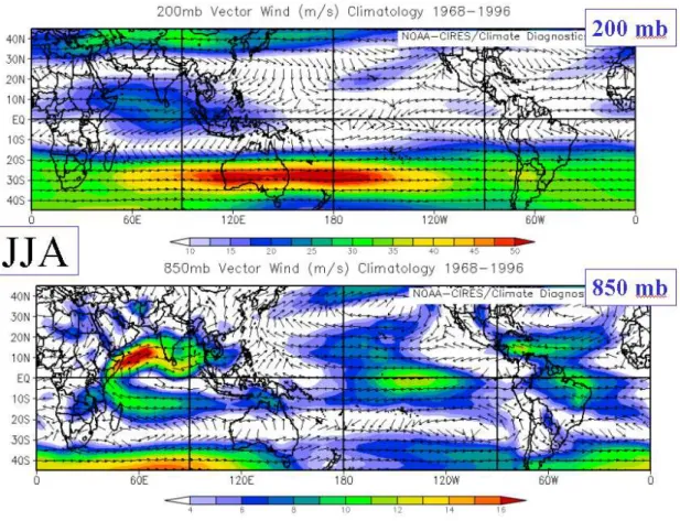
Figure 1.11 shows the mean wind distribution at 850 mb and 200 mb for JJA. These levels characterize the lower and upper troposphere, respectively. Similar diagrams for DJF are shown in Fig. 1.12. At a first glance, the flow patterns show a somewhat complicated structure, but careful inspection reveals some rather general features.

At 850 mb there is a cross-equatorial component of flow towards the summer hemisphere, especially in the Asian, Australian and (east) African sectors. This flow, which reverses between seasons, constitutes the planetary monsoons (see §1.8).

In the same sectors in the upper troposphere the flow is generally opposite to that at low levels, i.e., it is towards the winter hemisphere, with strong westerly winds (much stronger in the winter hemisphere) flanking the more meridional equatorial flow.

Both the upper and lower tropospheric flow in the Asian, Australian and African regions indicate the important effects of the land distribution in the tropics. Over the Pacific Ocean, the flow adopts a different character. At low levels it is generally eastward while at upper levels it is mostly westward. Thus the equatorial Pacific

(14)

CHAPTER 1. INTRODUCTION TO THE TROPICS 14 region is dominated by motions confined to a zonal plane. Note the strong easterly flow along the Equator in the central Pacific in both seasons. These are associated with the Walker circulation discussed below.

In JJA, the upper winds near the equator are mostly easterly, rather than westerly as suggested by Fig. 1.6. This is consistent with the fact that mean position of the upward branch of the Hadley circulation lies north of the Equator and, as shown below, it is dominated by the circulation in the Asian region. In DJF, the upper winds at the Equator are generally westerly in the eastern hemisphere and westerly in the western hemisphere.

Figure 1.11: Mean wind fields at 850 mb and 200 mb during JJA (Based on NCEP Reanalysis data).

In constructing zonally-averaged charts, an enormous amount of structure is

“averaged-out”. To expose some of this structure while still producing a simpler picture than the wind fields, we can separate the three-dimensional velocity field into a rotational part and a divergent part (see e.g. Holton, 1972, Appendix C).

Thus

V =k∧ ∇ψ− ∇χ (1.1)

(15)

Figure 1.12: As in Fig. 1.11, but for DJF.

where ψ is a streamfunction andχ a velocity potential. The contribution k∧ ∇ψ is rotational with∇∧(k∧∇ψ) =k∇²ψ, but nondivergent, whereas,∇χis irrotational, but has divergence ∇²χ. Because of this last property, examination of the velocity potential is especially useful as a diagnostic tool for isolating the divergent circulation.

It is this part of the circulation which responds directly to the large-scale heating and cooling of the atmosphere.

Figure 1.13 shows the distribution of the upper-tropospheric mean seasonal velocity potential χand arrows denoting the divergent part of the mean seasonal wind field during summer and winter. Two features dominate the picture. These are the large area of negative χ centred over southeast Asia in JJA and the equally strong negative region over Indonesia in DJF. These negative areas are located over positive χ centres at low levels (Krishnamurti, 1971, Krishnamurti et al., 1973)¹. Moreover, the two areas dominate all other features.

The wind vectors indicate distinct zonal flow in the equatorial belt over the Pacific

1Note that Krishnamurti definesχ to have the opposite sign to the normal mathematical convention used here. Accordingly, the signs in Fig. 1.13 have been changed to be consistent with our sign convention, the convention used also by the Australian Bureau of Meteorology.

(16)

Figure 1.13: Distribution of the upper tropospheric (200 mb) mean seasonal velocity potential (solid lines) and arrows indicating the divergent part of the mean seasonal wind which is proportional to ∇²χ. (Adapted from Krishnamurti et al., 1973).

and Indian Oceans and strong meridional flow northward into Asia and southward across Australia. The meridional flow is strongest in these sectors (i.e., in regions of strongest meridionally-orientated ∇χ ) and shows that the Hadley cell is actually dominated by regional flow at preferred longitudes.

When interpreting theχ-fields, a note of caution is appropriate. Remember that

∇ ·V =−∇²χand that |w|α|∇ ·V|. Therefore centres ofχ maximum or minimum do not coincide with centres of w maximum or minimum. The latter occur where

∇²χ is a maximum or minimum.

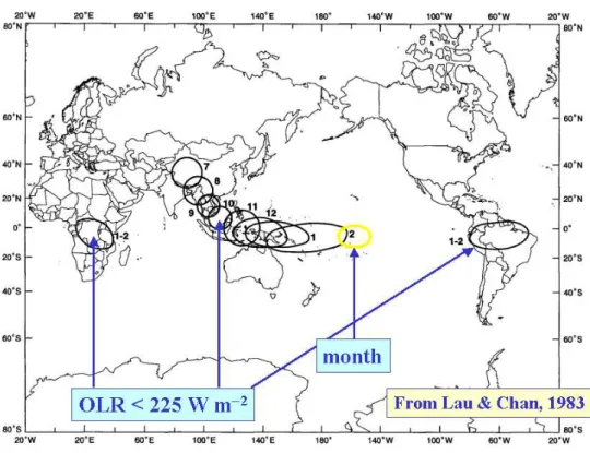
The seasonal changes in the broadscale upper-level divergence patterns indicated in Fig. 1.13 are reflected in the seasonal migration of the diabatic heat sources shown in Fig. 1.14. These heat sources are identified by regions of high cloudiness, itself characterized by regions with low values (<225 W m⁻²) of outgoing long-wave radiation (OLR) measured by satellites. The assumption is that high cloudiness (cold cloud tops) arises principally from deep convection heating and can be used as a proxy for this.

Krishnamurti’s arrows in Fig. 1.13 are also somewhat misleading as they refer only to the wind direction and not its magnitude. It is possible to study the flow in the equatorial belt by considering a zonal cross-section (longitude versus height) along the equator with the zonal and vertical components of velocity plotted. The mean circulation in such a cross-section is shown in Fig. 1.15. Strong ascending motion occurs in the western Pacific and Indonesian region with subsidence extending over most of the remaining equatorial belt. Exceptions are the small ascending zones

(17)

Figure 1.14: Seasonal migration of the diabatic heat sources during the latter half of the year (July-February, denoted by matching numerals). The extent of the diabatic heat sources is determined from the area with OLR values less than 225 W m⁻² from monthly OLR climatology and is approximately proportional to the size and orientation of the schematic drawings. (Adapted from Lau and Chan 1983)

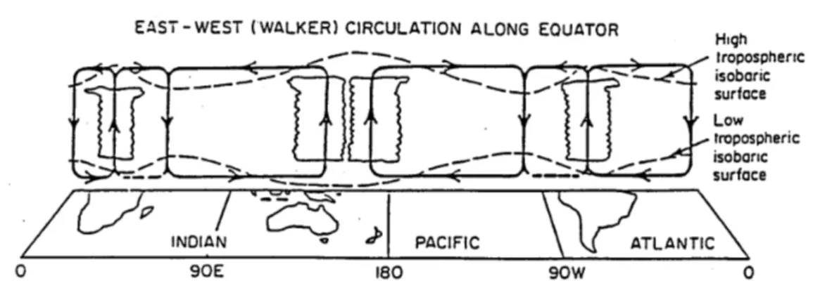
over South America and Africa. It should be noted that the Indonesian ascending region lies to the east of the velocity potential maximum in Fig. 1.13, in the area where ∇²χ is largest. The dominant east-west circulation is often called theWalker Circulation. Also plotted in Fig. 1.15 are the distributions of the pressure deviation in the upper and lower troposphere. These are consistent with the sense of the large-scale circulation, the flow being essentially down the pressure gradient.

Figure 1.15 displays significant vertical structure in the large scale velocity field.

Data indicate that the tropospheric wind field possesses two extrema: one in the upper troposphere and one in the lower troposphere. A theory of tropical motions will have to account for these large horizontal and vertical scales. Indeed, it is interesting to speculate on the reason for the large scale of the structures which dominate the tropical atmosphere. Their stationary nature, at least on seasonal time scales, suggests that they are probably forced motions, the forcing agent being the differential heating of the land and ocean or other forms of heating resulting from it.

There is a considerable amount of observational evidence to support the heating

(18)

Figure 1.15: Schematic diagram of the longitude-height circulation along the equator.

The surface and 200 mb pressure deviations are shown as dashed lines. Clouds indicate regions of convection. Note the predominance of the Pacific Ocean - Indonesian cell which is referred to as the Walker Circulation. (From Webster, 1983)

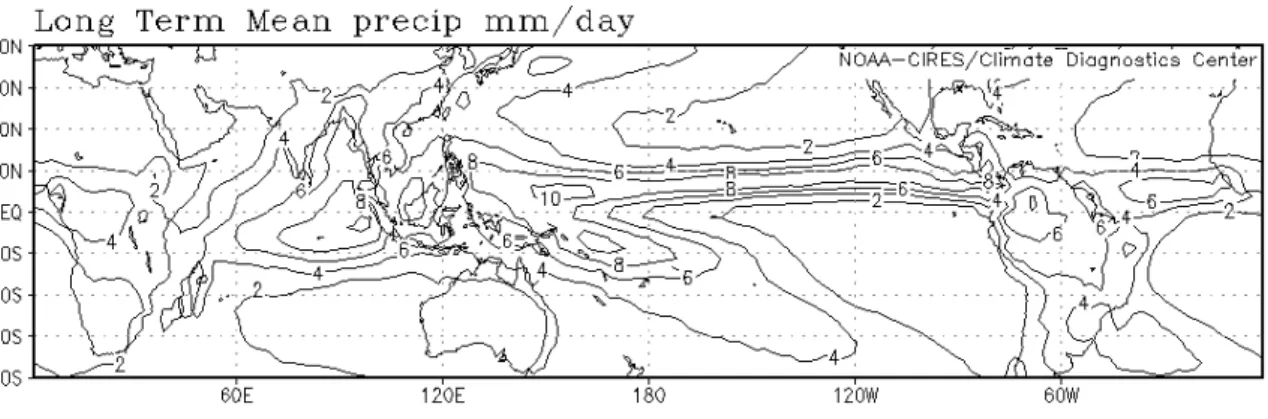
hypothesis. For example, Fig. 1.16 shows the distribution of annual rainfall throughout the tropics. It is noteworthy that the heaviest falls occur in the Indonesian and Southeast Asian region with a distribution which corresponds to the velocity potential field shown earlier. One is led to surmise that the common ascending branch of the Hadley cell and Walker cell is driven in some way by latent heat release. It is a separate problem to understand why the maximum latent heat release would be located in the Indonesian region. Figures 1.17 and 1.18 point to a solution. Figure 1.17 shows the distribution of mean annual surface air temperature. The pattern possesses considerable longitudinal variation, but correlates well with the sea surface temperature (SST) distribution shown in Fig. 1.18. Of great importance is the 8- 10^◦C longitudinal temperature gradient across the Pacific Ocean. The air mass over the western Pacific should be much more unstable to convection than that overlying the cooler waters of the eastern Pacific.

It is important to remember that the seasonal or annual mean fields shown above possesses both temporal and spatial variations on even longer time scales (see section 1.6). Figure 1.19 shows the mean annual temperature range of the air near sea level.

It is significant that in the equatorial belt, the temperature variations are generally very small, perhaps an order of magnitude smaller than those observed at higher latitudes. This is true for both land and sea areas. We may conclude that the variations with longitude shown earlier will be maintained. On the other hand, at higher latitudes, the near surface temperature over the sea possesses a relatively large amplitude variation which is surpassed only by the temperature variation over land. Figure 1.19 shows only the amplitude of the variation and gives no details of its phase. In fact, the ocean temperature at higher latitudes lags the insolation by some 2 months. Continental temperatures lag by only a few weeks.

(19)

Figure 1.16: Distribution of annual rainfall in the tropics. Contour values marked in cm/day.

Figure 1.17: Mean annual surface air temperature in the tropics (Units ^oC.

1.5 More on the Walker Circulation

Figure 1.20 shows a closer view of the Walker circulation with ascent over the warm pool region and subsidence over the cooler waters of the eastern Pacific. Over the Pacific the flow is easterly at low levels and westerly at upper levels. The term

“Walker Circulation” appears to have been first used by Bjerknes (1969) to refer to the overturning of the troposphere in the quadrant of the equatorial plane spanning the Pacific Ocean and it was Bjerknes who hypothesized that the “driving mechanism” for this overturning is condensational heating over the far western equatorial Pacific where SSTs are anomalously warm. The implication is that the source of precipitation associated with this driving mechanism is the local evaporation associated with the warm SSTs. This assumption was questioned by Cornejo-Garrido and Stone (1977) who showed on the basis of a budget study that the latent heat release driving the Walker Circulation is negatively-correlated with local evaporation, whereupon moisture convergence from other regions must be important. Newell et al. (1974) defined the Walker Circulation as the deviation of the circulation in the

(20)

Figure 1.18: Annual mean sea surface temperature in the tropics.

equatorial plane from the zonal average. Figure 1.21, taken from Newellet al., shows the contours of zonal mass flux averaged over the three month period December 1962 - February 1963 in a 10^◦S wide strip centred on the equator. In this representation there are five separate circulation cells visible around the globe, but the double cell whose upward branch lies over the far western Pacific is the dominant one. A similar diagram for the northern summer period June to August (Fig. 1.21(b)) shows only three cells, but again the major rising branch lies over the western Pacific. As we shall see, the circulation undergoes significant fluctuations on both interannual (1.6) and intraseasonal (1.7) time scales.

1.6 El Ni˜ no and the Southern Oscillation

There is considerable interannual variability in the scale and intensity of the Walker Circulation, which is manifest in the so-called Southern Oscillation (SO). The latter is associated with fluctuations in sea level pressure in the tropics, monsoon rainfall, and the wintertime circulation over the Pacific Ocean. It is associated also with fluctuations in circulation patterns over North America and other parts of the extratropics. Indeed, it is the single most prominent signal in year-to-year climate variability in the atmosphere. The SO was first described in a series of papers in the 1920s by Sir Gilbert Walker (Walker, 1923, 1924, 1928) and a review and refer- ences are contained in a paper by Julian and Chervin (1978). The latter authors use Walkers own words to summarize the phenomenon. “By the southern oscillation is

(21)

Figure 1.19: Mean annual temperature range (^◦C) of the air near sea level.

(22)

Figure 1.20: A close-up view of the Walker circulation showing ascent over the warm pool region and subsidence over the cooler waters of the eastern Pacific. The flow is easterly at low levels and westerly at upper levels.

implied the tendency of (surface) pressure at stations in the Pacific (San Francisco, Tokyo, Honolulu, Samoa and South America), and of rainfall in India and Java...

to increase, while pressure in the region of the Indian Ocean (Cairo, N.W. India, Darwin, Mauritius, S.E. Australia and the Cape) decreases...” and “We can perhaps best sum up the situation by saying that there is a swaying of pressure on a big scale backwards and forwards between the Pacific and Indian Oceans...”.

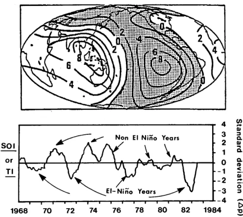
Figure 1.22a depicts regions of the globe affected by the SO. It shows the simultaneous correlation of surface pressure variations at all places with the Darwin surface pressure. It is clear, indeed, that the “sloshing” back and forth of pressure which characterizes the SO does influence a very large area of the globe and that the “centres of action”, namely Indonesia and the eastern Pacific, are large also.

Figure 1.22b shows the variation of the normalized Tahiti-Darwin pressure anomaly difference, frequently used as a Southern Oscillation Index (SOI), which gives an indication of the temporal variation of the phase of the SO. For example, a positive SOI means that pressures over Indonesia are relatively low compared with those over the eastern Pacific and vice versa.

It was Bjerknes (1969) who first pointed to an association between the SO and the Walker Circulation, although the seeds for this association were present in the investigations by Troup (1965). These drew attention to the presence of interannual changes in the upper troposphere flow over the tropics associated with the SO and indicated that the anomalies in the flow covered a large range of longitudes. Bjerknes stated:

“The Walker Circulation. . . must be part of the mechanism of the still

larger ‘Southern Oscillation’ statistically defined by Sir Gilbert Walker. . . whereas

(23)

(a)

(b)

Figure 1.21: Deviations of the zonal mass flux, averaged over the latitude belt 0^◦- 10^◦N, from the zonal mean. for the periods (a) December - February, and (b) June - August calculated by Newell et al. (1974). Contours do not correspond with streamlines, but give a fairly good representation of the velocity field associated with the Walker Circulation.

the Walker Circulation maintains east-west exchange of air covering a little over an earth quadrant of the equatorial belt from South America to the west Pacific, the concept of the Southern Oscillation refers to the barometrically-recorded exchange of mass along the complete circumfer- ence of the globe in tropical latitudes. What distinguishes the Walker Circulation from other tropical east-west exchanges of air is that it oper-

(24)

Figure 1.22: The spatial variation of the simultaneous correlation of surface pressure variations at all points with the Darwin surface pressure (upper panel). Shaded areas show negative correlations. The lower panel shows the variation of the normalized Tahiti-Darwin pressure difference on the Southern Oscillation Index. (From Webster, 1987b)

ates a large tapping of potential energy by combining the large-scale rise of warm-moist air and descent of colder dry air”.

In a subsequent paper, Bjerknes (1970) describes this thermally-direct circulation oriented in a zonal plane by reference to mean monthly wind soundings at opposing

“swings” of the SO and the patterns of ocean temperature anomalies.

El Ni˜no is the name given to the appearance of anomalously warm surface water off the South American coast, a condition which leads periodically to catastrophic downturns in the Peruvian fishing industry by severely reducing the catch. The colder water that normally upwells along the Peruvian coast is rich in nutrients, in contrast to the warmer surface waters during El Ni˜no. The phenomenon has been the subject of research by oceanographers for many years, but again it seems to have been Bjerknes (1969) who was the first to link it with the SO as some kind of air- sea interaction effect. Bjerknes used satellite imagery to define the region of heavy rainfall over the zone of the equatorial central and eastern Pacific during episodes

(25)

CHAPTER 1. INTRODUCTION TO THE TROPICS 25 of warm SSTs there. He showed that these fluctuations in SST and rainfall are associated with large-scale variations in the equatorial trade wind systems, which in turn affect the major variations of the SO pressure pattern. The fluctuations in the strength of the trade winds can be expected to affect the ocean currents, themselves, and therefore the ocean temperatures to the extent that these are determined by the advection of cooler or warmer bodies of water to a particular locality, or, perhaps more importantly to changes in the pattern of upwelling of deeper and cooler water.

Figure 1.23 shows time-series of various oceanic and atmospheric variables at tropical stations during the period 1950 to 1973 taken from Julian and Chervin (1978).

These data include the strength of the South Equatorial Current; the average SST over the equatorial eastern Pacific; the Puerto Chicama (Peru) monthly SST anomalies; the 12 month running averages of the Easter Island-Darwin differences in sea level pressure; and the smoothed Santiago-Darwin station pressure differences. The figure shows also the zonal wind anomalies at Canton Island (3^◦S, 172^◦W) which was available for the period 1954-1967 only. The mutual correlation and particular phase association of these time series is striking and indicate an atmosphere-ocean coupling with a time scale of years and a spatial scale of tens of thousands of kilometres in- volving the tropics as well as parts of the subtropics. This coupled ocean-atmosphere phenomenon is now referred to as ENSO, an acronym forEl Ni˜no-Southern Oscilla- tion.

During El Ni˜no episodes, the equatorial waters in the eastern half of the Pacific are warmer than normal while SSTs west of the date line are near or slightly below normal. Then the east-west temperature gradient is diminished and waters near the date line may be as warm as those anywhere to the west (∼ 29^◦C). The region of heavy rainfall, normally over Indonesia, shifts eastwards so that Indonesia and adjacent regions experience drought while the islands in the equatorial central Pacific experience month after month of torrential rainfall. Near and to the west of the date line the usual easterly surface winds along the equator weaken or shift westerly (with implication for ocean dynamics), while anomalously strong easterlies are observed at the cirrus cloud level. In essence, in the atmosphere there is an eastward displacement of the Walker Circulation.

There are various theories for the oceanic response to changes in the atmospheric circulation, but as yet none is widely accepted as the correct one. A brief review of these is given by Hirst (1989). A popular style review of the meteorological aspects of ENSO is given by Rasmussen and Wallace (1983), who discuss, inter alia, the implications of ENSO for circulation changes in middle and higher latitudes. A more recent review is that of Philander (1990).

1.7 The Madden-Julian/Intraseasonal Oscillation

As well as fluctuations on an interannual basis, the Walker Circulation appears to undergo significant fluctuations on intraseasonal time scales. This discovery dates back to pioneering studies by Madden and Julian (1971, 1972) who found a 40-50

(26)

Figure 1.23: Composite low-pass filtered time series for various oceanographic and meteorological parameters involved in the Southern Oscillation and Walker- Circulation. Series are (top to bottom): the strength of the South Equatorial Cur- rent, a westward flowing current just south of the equator; ocean surface temperature anomalies in the region 5^◦N-5^◦S and 80^◦W to 180^◦W (solid line), and monthly anomalies of Puerto Chicama ocean surface temperature, dashed; two Southern Oscillation indices, the dashed line being 12-month running means of the difference in station pressure Easter Island-Darwin and the solid line being a similar quantity except San- tiago is used instead of Easter Island; the bottom series are low-pass filtered zonal wind anomalies (from monthly means) at Canton at 850 mb (dashed) and 200 mb (solid). The short horizontal marks appearing between two panels denote the aver- aging intervals used in compositing variables in cold water and El Ni˜no situations.

(From Julian and Chervin, 1978)

day oscillation in time series of sea-level pressure and rawinsonde data at tropical stations. They described the oscillation as consisting of global-scale eastward- propagating zonal circulation cells along the equator. The oscillation appears to be associated with intraseasonal variations in tropical convective activity as evidenced in time series of rainfall and in analyses of anomalies in cloudiness and OLR.

The results of various studies to the mid-80s are summarized by Lau and Peng (1987). They list the key features of the intraseasonal variability as follows:

(27)

CHAPTER 1. INTRODUCTION TO THE TROPICS 27 i. There is a predominance of low-frequency oscillations in the broad range from

30-60 days;

ii. The oscillations have predominant zonal scales of wavenumbers 1 and 2 and propagate eastward along the equator year-round.

iii. Strong convection is confined to the equatorial regions of the Indian Ocean and western Pacific sector, while the wind pattern appears to propagate around the globe.

iv. There is a marked northward propagation of the disturbance over India and East Africa during summer monsoon season and, to a lesser extent, southward penetration over northern Australia during the southern summer.

v. Coherent fluctuations between extratropical circulation anomalies and the tropical 40-50 day oscillation may exist, indicating possible tropical-midlatitude interactions on the above time scale.

vi. The 40-50 day oscillation appears to be phase-locked to oscillations of 10-20 day periods over India and the western Pacific. Both are closely related to monsoon onset and break conditions over the above regions.

Figure 1.24 shows a schematic depiction of the time and space variations of the circulation cells in a zonal plane associated with the 40-50 day oscillation as envisaged by Madden and Julian (1972).

Figure 1.25 shows the eastward propagation of the 40-50 day wave in terms of its velocity potential in the Eastern Hemisphere. The four panels, each separated by five days, show the distributions of the velocity potential at 850 mb. The centre of the ascending (descending) region of the wave is denoted by A (B). As the wave moves eastwards, it intensifies as shown by the increased gradient. Furthermore, and very important, as centre A moves eastwards from the southwest of India (which lies between 70^◦E and 90^◦E) to the east of India, the direction of the divergent wind over India changes from easterly to westerly. Notice also that as centre A moves across the Indian region that the gradient of velocity potential intensifies to the north as indicated by the movement of the stippled regions in panels 2 and 3. Thus, depending on where the centres A and B are located relative to the monsoon flow, the strength of the monsoon southwesterlies flowing towards the heated Asian continent will be strengthened or weakened. Thus we can the importance of the phase of the MJO on the mean monsoonal flow.

According to Lau and Peng, the most fundamental features of the oscillation are the perennial eastward propagation along the equator and the slow time scale in the range 30-60 days. To date, observational knowledge of the phenomenon has outpaced theoretical understanding, but it would appear that the equatorial wave modes to be discussed in Chapter 3 play an important role in the dynamics of the oscillation.

Furthermore, because of the similar spatial and relative temporal evolution of atmospheric anomalies associated with the 40-50 day oscillation and those with ENSO, it

(28)

Figure 1.24: (a) Schematic depiction of the time and space variations of the disturbance associated with the 40-50 day oscillation along the equator. The times of the cycles (days) are shown to the left of the panels. Clouds depict regions of enhanced large-scale convection. The mean disturbance pressure is plotted at the bottom of each panel. The circulation on days 10-15 is quite similar to the Walker circulation shown in Fig. 1.15. The relative tropopause height is indicated at the top of each panel. (b) shows the mean annual SST distribution along the equator. The 40-50 day wave appears strongly convective when the SST is greater than 27^◦C as in panels 2-5 in (a). Panel (c) shows the variations of pressure difference between Darwin and Tahiti. The swing is reminiscent of the SO, but with a time scale of tens of days rather than years. (From Webster, 1987b)

is likely that the two phenomena are closely related (see. e.g. Lau and Chan, 1986).

Indeed, one might view the atmospheric part of the ENSO cycle as fluctuations in a longer-term (e.g. seasonal average of the MJO). Two recent observational studies of

(29)

Figure 1.25: (a) The latitude-longitude structure of the 40-50 day wave in the Eastern Hemisphere in terms of 850 mb velocity potential. Units 10⁻⁶ s⁻¹. The arrows denote the direction of the divergent part of the wind and the stippled region the locations of maximum speed associated with the wave. Letters A and B depict the centres of velocity potential, which are seen to move eastwards. Centre A may be thought of as a region of rising air and B a region of subsidence. (From Webster 1987b)

the MJO are those of Knutson et al., (1986) and Knutson and Weickmann (1987).

A recent review of theoretical studies is included in the paper by Blad´e and Hart- mann (1993) and a recent reviews of observational studies are contained in papers by Madden and Julian (1994) and Yanai et al. (2000).

One might view the Walker Circulation as portrayed in Figs. 1.15 and 1.21 as an average of several cycles of the MJO.

1.8 More on Monsoons

The term monsoon originates from the Arabic “Mausim”, a season, and was used to describe the change in the wind regimes as the northeasterlies retreated to be replaced by the southwesterlies or vice versa. The term will be used here to describe the westerly air stream (southwesterly in the NH, northwesterly in the SH) that results as the trade winds cross the equator and flow into the equatorial trough.

Accordingly, the term refers to the wind regime and not to areas of continuous rain etc., which are associated with the monsoon. Figure 1.27 shows the typical low-level flow and other smaller scale features associated with the (NH) summer and winter

(30)

CHAPTER 1. INTRODUCTION TO THE TROPICS 30 monsoons in the Asian regions.

Figure 1.26: Schematic of low-level air flow patterns near the Equator in January and July showing the main regions of cross equatorial flow in the monsoon regions.

Two main theories have been advanced to account for the monsoonal perturbations.

1.8.1 The Regional Theory

This regards the monsoon perturbations as low-level circulation changes resulting entirely from the large-scale heating and cooling of the continents relative to oceanic regions. In essence the monsoon is considered as a continental scale “sea breeze”

where air diverges away from the cold winter continents and converges into the heat lows in the hot summer continents. The flow at higher levels is assumed to play a minor role.

1.8.2 The Planetary Theory

With the great increase in upper air observations during the second half of this century, marked changes in the upper tropospheric flow patterns have been found to accompany the onset of monsoonal conditions in the lower levels. In particular, marked changes in the position of the subtropical jet stream accompany the advance of the monsoonal winds.

There are several objections to the regional theory. For example, monsoonal circulations are observed over the oceans, well removed from any land mass, and the heat low over the continents is often remote from the main monsoonal trough. More- over, the seasonal displacement of surface and upper air features is well established from mean wind charts. This displacement is on a global scale, but is greatest over the continental land masses, especially the extensive Asian continent. Hence an understanding of planetary circulation changes in conjunction with major continental perturbations is necessary in understanding the details of the monsoonal flow.

(31)

Figure 1.27: Air flow patterns and primary synoptic- and smaller scale features that affect cloudiness and precipitation in the region of (a) the summer monsoon, and (b) the winter monsoon. In (a), locations of June to September rainfall exceeding 100 cm the land west of 100^◦E associated with the southwest monsoon are indicated.

Those over water areas and east of 100^◦E are omitted. In (b) the area covered by the ship array during the winter MONEX experiment is indicated by an inverted triangle. (From Houze, 1987)

1.9 Monsoon variability

Superimposed upon the seasonal cycle are significant variations in the weather of the tropical regions. For example, in the monsoon regions the established summer mon-

(32)

CHAPTER 1. INTRODUCTION TO THE TROPICS 32 soon undergoes substantial variations, vacillating between extremely active periods and distinct “lulls” in precipitation. The latter are referred to as “monsoon breaks”.

An example of this form of variability is shown in Fig 1.28 which summarizes the monsoon rains of two years, 1963 and 1971, along the west coast of India. The

“active periods” are associated with groups of disturbances and the “breaks” with an absence of them,. Usually, during the break, precipitation occurs far to the south of India and also to the north along the foothills of the Himalaya. Such variability as this appears characteristic of the precipitating regions of the summer and winter phases of the Asian monsoon and the African monsoon.

Figure 1.28: Daily rainfall (cm/day) along the western coast of India incorporating the districts of Kunkan, Coastal Mysore and Kerala for the summers of 1963 and 1971. (From Webster, 1983)

(33)

1.10 Synoptic-scale disturbances

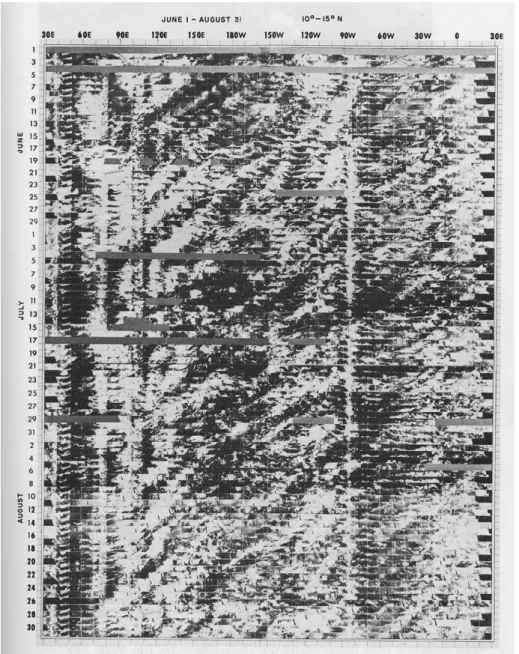
The individual disturbances of the active monsoon and those associated with the near- equatorial troughs move westward in a fairly uniform manner. Such movement is shown clearly in Fig. 1.29. The westward movement is apparent in the bands of cloudiness extending diagonally from right to left across the time-longitude sections.

Figure 1.29: Time-longitude section of visible satellite imagery for the latitude band 10-15^◦N of the tropics. Cloud streaks moving from right to left with increasing time denotes westward propagation. Note that there is typically easterly flow at these latitudes. (From Wallace, 1970)

(34)

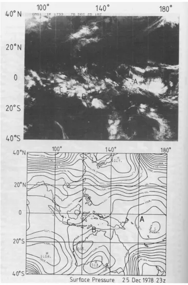
CHAPTER 1. INTRODUCTION TO THE TROPICS 34 To illustrate the structure of propagating disturbances, Webster (1983) discusses a particular example taken from Winter-MONEX) in 1978. Figure 1.30 shows the Japanese geostationary satellite (GMS) infra-red (IR) satellite picture at 1800 UTC on 25 December 1978 for the Winter-MONEX region with the .2300 UTC surface pressure analysis underneath. Figure 1.31 shows the corresponding wind fields at 250 mb and 950 mb. What is striking is the existence of significant structures in the satellite cloud field which have no obvious signature in the surface pressure field.

Indeed, the tropical portion of the pressure field is relatively featureless, except for the heat low in north-western Australia and the broad trough that spans the near equatorial region of the southern hemisphere just west of the date line. The most that one can say is that the major cloud regions appear to reside about the axis of a broad equatorial trough.

Webster considers three major regions of deep high cloudiness denoted by A, B and C which appear to be synoptic scale disturbances. He shows that these can be associated with areas of low-level convergence in the 950 mb wind field lying beneath areas of upper-level divergence at 200 mb. The implication is that these are each deep divergent systems. Such properties: lower tropospheric convergence, deep penetrative convection and upper-level divergence appear characteristic of the synoptic-scale tropical disturbances of the ITCZ and the major convective zones of the monsoon.

Figure 1.32 shows the surface pressure trace for Darwin from 23 - 28 December 1978, covering the period of the case study presented in Figs. 1.29 and 1.30. The major variation in the pressure is associated with the semi-diurnal oscillation which has an amplitude of about 4 mb. Little alteration to the semi-diurnal trend is apparent near 25 December 1978 which coincides with the existence there of the disturbance. Indeed at low latitudes only on rare occasions with the passage of a tropical cyclone will the synoptic-scale pressure perturbations be larger than the semi-diurnal variation.

(35)

Figure 1.30: The winter MONEX region of 25 December 1978. Upper panel shows the GMS IR satellite picture with the surface-pressure pattern shown on lower panel.

Both panels are on the same projection. Pressure analysis after McAvaney et al.

(1981): Letters A. B and C identify synoptic-scale disturbances referred to in the text. (From Webster, 1983)

(36)

Figure 1.31: The 250 mb (upper panel) and 950 mb (lower panel) wind fields for the winter MONEX region of 25 December 1978 with the horizontal wind divergence superimposed in the 20^◦N - 20^◦S latitude strip. In the upper troposphere areas the divergence are stippled whereas in the lower troposphere areas of convergence are stippled. Stippled areas denote divergence magnitudes greater than 50×10⁻⁵s⁻¹. (From Webster, 1983)

(37)

Figure 1.32: The variation of surface pressure at Darwin for the period 23 - 28 December 1978. The structure is dominated by the semi-diurnal atmospheric tide.

(38)

Chapter 2 EQUATIONS AND SCALING AT LOW LATITUDES

The governing equations of atmospheric and oceanic motion are intrinsically complicated, a reflection of the myriad of time and space scales they represent. Therefore, in order to study a specific phenomenon it is desirable to simplify the equations by a scale analysis, removing those terms which are unimportant for the phenomenon in question. The scaling to be described here is incomplete, but is aimed at comparing the dominant processes at low and higher latitudes. A scale analysis for midlatitude synoptic systems is described in DM, Chapter 3.

2.1 The governing equations on a sphere

The basic equations for the motion of a dry atmosphere are ρDu

Dt =−∇p+ρg−ρΩ∧ u+F, (2.1)

Dρ

Dt =−ρ∇ ·u, (2.2)

cp

D

Dtlnθ = Q

T, (2.3)

p=ρ RT. (2.4)

The first three represent the conservation of momentum, the conservation of mass and the conservation of energy (first law of thermodynamics), respectively;

the last is the equation of state. The variables u, p, ρ, T and θ and Q represent the (three-dimensional) fluid velocity, total pressure, density, temperature, potential temperature, and diabatic heating rate, respectively; F represents viscous and or turbulent stresses, and g is theeffective gravity. The potential temperature is related

38

(39)

CHAPTER 2. EQUATIONS AND SCALING AT LOW LATITUDES 39 to the temperature and pressure by the formula θ =T(p^∗/p)^κ, wherep^∗ = 1000 mb and κ = 0.2865.

The shape of the earths surface is approximately an oblate spheroid with an equatorial radius of 6378 km and a polar radius of 6357 km. The surface is close to a geopotential surface, i.e. a surface which is perpendicular to the effective gravity (see DM, Chapter 3). As far as geometry is concerned the equations of motion can be expressed with sufficient accuracy in a spherical coordinate system (λ, φ, r), the components of which represent longitude, latitude and radial distance from the centre of the earth (see Fig. 2.1). The coordinate system rotates with the earth at an angular rate Ω =|Ω|= 7.292×10⁻⁵ rad s⁻¹. An important dynamical requirement in the approximation to a sphere is that the effective gravity appears only in the radial equation of motion, i.e. we regard spherical surfaces as exact geopotentials so that the effective gravity has no equatorial component. Further details are found in Gill (1982; 4.12).

Alternatively, the equations may be written in coordinates (λ, φ, z), where z is the height above the earths surface (or more precisely the geopotential height). Note that r = a+z, where a is the earths radius. Since the atmosphere is very shallow compared with its radius (99% of the mass of the atmosphere lies below 30 km, whereas a = 6367 km), we may approximate r by a and replace ∂/∂r by ∂/∂z. In (λ, φ, z) coordinates, the frictionless forms of Eqs. (2.1) and (2.2) are (Holton, 1979, p 35)

Figure 2.1: The (λ, φ, z) coordinate system

(40)

CHAPTER 2. EQUATIONS AND SCALING AT LOW LATITUDES 40

Du

Dt − uvtanφ a +uw

a∗

=− 1

ρacosφ

∂p

∂λ + 2Ω vsinφ−2Ω w

∗ cosφ, (2.5) Dv

Dt +u²tanφ a +vw

a∗

=− 1 ρa

∂p

∂φ −2Ω usinφ, (2.6)

Dw

Dt − u²+v² a∗

=−1 ρ

∂p

∂z −g+ 2Ωu

∗ cosφ, (2.7)

Dρ

Dt =− ρ acosφ

∂u

∂λ + ∂

∂φ (vcosφ)

−ρ∂w

∂z −2ρw a∗

, (2.8)

where u = a cosφ^dλ_dti+r^dφ_dtj+^dz_dtk = ui+vj+wk. Here u, v and w represent the eastward, northward and vertical components of velocity, and _Dt^D ≡ ∂t^∂ +u· ∇, is the total-, or Lagrangian-, or material- derivative, following an air parcel. The terms with an asterisk beneath them will be referred to later.

2.2 The hydrostatic equation at low latitudes

In Chapter 1 we discussed the enormous diversity of motion scales which exists in low latitudes. We explore now the range of scales for which we may treat the motion as hydrostatic.

To carry out a scaling of (2.7) it is convenient to define a reference density and pressure, ρ0(z) and p0(z), characteristic of the tropical atmosphere and to define a perturbation pressure p^′ as the deviation of p from p0(z). Then −g in Eq. (2.7) must be replaced by the buoyancy force per unit mass, σ =−g(ρ−ρ0(z))/ρ, andp may be replaced by p^′ in Eqs. (2.5) and (2.6). Details may be found in DM, Ch. 3.

Omitting primes, (2.7) may be written Dw

Dt +1 ρ

∂p

∂z −σ= u²+v²

a + 2Ωucosφ. (2.9)

To perform the necessary scale analysis we let U, W, L, D, δp,Σ and τ represent typical horizontal and vertical velocity scales, horizontal and vertical length scales, a pressure deviation scale, a buoyancy scale and a time scale for the motion of a particular atmospheric system. The terms in (2.9) then have scales

W τ

δp

ρD Σ U²

a 2ΩU (2.10)

For a value ofδp≈1 mb (10²Pa) over the troposphere depth (20 km),δp/(ρD)≈ 10² ÷(1.0×2.0×10⁴) = 0.5×10⁻² m s⁻². Also for U ≈ 10 m s⁻¹, Ω ≈ 10⁻⁵ s⁻¹ and a≈6×10⁶ m, the last two terms are of the order of 10⁻⁴ and can be neglected.

(41)

CHAPTER 2. EQUATIONS AND SCALING AT LOW LATITUDES 41 The principal question is whether the vertical acceleration term can be neglected compared with the vertical pressure gradient per unit mass. To investigate this consider

Dw Dt /

1 ρ

∂p

∂z

≈ W

τ / 1

ρ δp D

. (2.11)

We obtain an estimate for δp from the horizontal equation of motion (2.1). This yields two possible scales, depending on whether the motion is quasi-geostrophic, i.e.

1/τ << f, or whether inertial effects predominate, 1/τ >> f. In the latter case (f τ <<1),

δp≈P1 =ρLU/τ; while in the former case (1<< f τ)

δp ≈P2 =ρLUf.

If 1/τ = f, then, of course, δp ≈ P1 = P2. With the foregoing scales for P we can calculate the ratio in (2.11). Using P1 we find that

W τ /1

ρ P1

D = W U

D L

Thus in the high frequency limit (f τ << 1), hydrostatic balance will occur if W << U and/or D/L << 1, provided that the other ratio is no more than O(1).

As we shall see later, this allows gravity waves to be treated hydrostatically, but the approximation is not valid for cumulus clouds.

In the low frequency limit (1<< f τ) we use P2, and obtain W

τ /1 ρ

P₂ D = W

U D L τ f.

Now, even ifW ≈U and D≈L, the hydrostatic approximation is justified provided 1 << f τ; which was the approximation that allowed us to obtain P anyhow. For synoptic-scale (L ≈ 10⁶), or planetary-scale (L ≈ a) motions, for both of which L >> D, the hydrostatic approximation is valid even if 1/τ ≈ f, and therefore as f decreases towards the equator. Thus we are well justified in treating planetary motions as hydrostatic.

We must be careful, however. We note that (2.5) has a component of the Coriolis force that is a maximum at the equator, i.e. although 2Ωvsinφ → 0 as φ → 0, 2Ωwcosφ → 2Ωw. But in invoking the hydrostatic approximation we neglect the term 2Ωucosφin (2.7). Thus forming the total kinetic energy equation with our new hydrostatic set we will produce an inconsistency. It appears in the following manner.

Multiplying (2.5) ×u, (2.6) ×v and (2.7) ×w and adding, we obtain

(42)

D Dt

1

2 u²+v²+w²

=−1 ρ

u acos φ

∂p

∂λ +v a

∂p

∂φ +w∂p

∂z

−gw. (2.12) We notice that all geometric terms and Coriolis terms have vanished by cancel- lation between the equations. This is as it should be as these terms are products of the geometry or are a consequence of Newtons second law being expressed in an accelerating frame of reference. That is, the terms would not appear as forces in an inertial frame and may not change the kinetic energy of the system.

The problem is: if we make the assumption that the system is hydrostatic and note that for large scale flow, |w| << |u|,|v|, then the total kinetic energy may be written as

1 2

D

Dt u²+v²

=−1 ρ

u acosφ

∂p

∂λ + v a

∂p

∂φ

−

2Ωuwcosφ−

u²+v² a

w

. (2.13) The last term in square brackets represents a fictitious or spurious energy source that arises from the lack of consistency in scaling the system of equations. Since each equation is interrelated to the others, it is incorrect to scale one without consideration of the others. Therefore, if the hydrostatic equation is used, energetic consistency requires that certain curvature and Coriolis terms must be omitted also. These are the terms marked underneath by a star in Eqs. (2.5) - (2.8). Similar considerations to these are necessary when “sound - proofing” the equations (see e.g. ADM, Ch.

2).

The hydrostatic formulation of the momentum equations with friction terms included then becomes

Du

Dt =− 1 ρacosφ

∂p

∂λ +

2Ω + u acosφ

vsinφ+Fλ, (2.14) Dv

Dt =− 1 ρa

∂p

∂φ −

2Ω + u acosφ

usinφ+Fφ, (2.15) 0 =−1

ρ

∂p

∂z −g. (2.16)

The need to neglect certain terms in the u and v equations to preserve energetic consistency has not been always appreciated. Many early numerical models, which were hydrostatic, could not conserve the total energy (i.e. kinetic and potential energy). The problem was traced to the inconsistency noted above.

2.3 Scaling at low latitudes

We consider now a more formal scaling of the hydrostatic equations in the vector form

(43)

∂

∂t +V· ∇^h

V+w ∂

∂z V+f k∧ V = −(1/ρ) ∇^hp (2.17) 0 =−1

ρ

∂p

∂z −g (2.18)

∂

∂t +V· ∇^h

ρ+ρ∇^h·V+ ∂

∂z (ρw) = 0 (2.19)

∂

∂t +V· ∇^h

lnθ+w ∂

∂zlnθ =Q/(cpT). (2.20) Here V is the horizontal wind vector, w the vertical velocity component and ∇^h is the horizontal gradient operator. We recognize that perturbations of pressure and density from the basic state p0(z), ρ0(z) are relatively small, but seek to estimate their sizes for low- and middle-latitude scalings in terms of flow parameters.

We define a pressure height scale Hp such that 1/Hp = −(1/p0)(dp0/dz) and note that, using the hydrostatic equation for the basic reference state, Hp =p0/gρ0. With quasi-geostrophic scaling appropriate to middle-latitudes, Eq. (2.17) gives δp ≈ρ0f UL, whereupon

δp

p₀ ≈ f UL gH_p = F²

Ro

Ro <<1 (2.21)

where Ro = _{f L}^U is the Rossby number, and

F = _(gH^U

p)¹^/² is aFroude number.

Note that (2.21) is satisfied even if Ro ≈1, because δp ≈ ρ0f UL then provides the same scale as the inertial scale δp≈ρ0U².

Hydrostatic balance expressed by (2.18) implies hydrostatic balance of the perturbation from the basic state, i.e. ∂p^′/∂z = −gρ^′, whereupon it follows that δp/D≈gδρ, and therefore

δρ

ρ0 ≈ δp

gDρ0 ≈ δp p0

Hs

D

≈ δp p0

= F² Ro

Ro <<1, (2.22) assuming D≈Hp.

Finally, since from the definition of θ, (1−κ)lnp=lnρ+lnθ + constant, δθ

θ₀ ≈ −κδp p₀ ≈ F²

Ro

Ro <<1. (2.23)

(44)

CHAPTER 2. EQUATIONS AND SCALING AT LOW LATITUDES 44 Typically, g ≈ 10 ms⁻², H_p ≈ 10⁴ m whereupon, for U ≈ 10 ms⁻¹, f ≈ 10⁻⁴ s⁻¹(a middle-latitude value), Ro = 0.1 and F² = 10⁻³. It follows that in middle latitudes,

δρ ρ0 ≈ δp

p0 ≈ δθ

θ0 ≈10⁻², (2.24)

confirming that for geostrophic motions, fluctuations in p, ρ and θ may be treated as small.

At low latitudes, f ≈ 10⁻⁵ s⁻¹ so that for the same scales of motion as above, Ro = 1. In this case, advection terms in (2.17) are comparable with the horizontal pressure gradient. However, as we have seen, the foregoing scalings remain valid for Ro≈1 and therefore

δρ ρ0 ≈ δp

p0 ≈ δθ

θ0 ≈10⁻³. (2.25)

Accordingly, we can expect fluctuations inp,ρandθto be an order of magnitude smaller in the tropics than in middle latitudes. The comparative smallness of the low-latitude perturbation may be associated with of the rapidity of the adjustment of the tropical motions to a pressure gradient imbalance; the adjustment being less constrained by rotational effects than at higher latitudes.

Consider now the adiabatic form of (2.20), i.e., put Q = 0. The scaling of this equation implies that

U L

δθ

θ0 ≈W 1 θ0

dθ₀ dz . Using (2.23) and defining

N² = g θ0

dθ0

dz , where N is the buoyancy frequency and,

Ri= N²H_p² U² , is a Richardson number, we have

U L

F²

Ro ≈WN²

g , or W ≈ UD L

1

Ro Ri, (2.26)

an estimate that is valid for Ro = 1. It follows that, for the same scales of motion and in the absence of convective processes of substantial magnitude, we may expect the vertical velocity in the equatorial regions to be considerably smaller than in the middle latitudes. For example, for typical scalesU = 10 ms⁻¹ ,D= 10 km,L= 1000 km, Hp = 10 km, N = 10⁻² s⁻¹,Ri = 10² and W = 10⁻³/Ro ms⁻¹. In the tropics, Ro ≈ 1 so that (2.26) would imply vertical velocities on the order of 10⁻³ ms⁻¹, which is exceedingly tiny.