on the representation of the sea surface temperature in the South Eastern Tropical Atlantic

(1)

https://doi.org/10.1007/s00382-020-05256-9

On the impact of atmospheric vs oceanic resolutions

on the representation of the sea surface temperature in the South Eastern Tropical Atlantic

Alba de la Vara^1,2 · William Cabos³ · Dmitry V. Sein^4,9 · Dmitry Sidorenko⁴ · Nikolay V. Koldunov^4,5 · Shunya Koseki⁶ · Pedro M. M. Soares⁷ · Sergey Danilov^4,8

Received: 10 January 2019 / Accepted: 15 April 2020 / Published online: 23 April 2020

Abstract

Despite the efforts of the modelling community to improve the representation of the sea surface temperature (SST) over the South Eastern Tropical Atlantic, warm biases still persist. In this work we use four different configurations of the fully- coupled AWI Climate Model (AWI-CM) which allow us to gain physics-based insight into the role of the oceanic and atmospheric resolutions of the model in the regional distribution of the SST. Our results show that a sole refinement of the oceanic resolution reduces warm biases further than a single increase of the atmospheric component. An increased oceanic resolution is required (i) to simulate properly the Agulhas Current and its associated rings; (ii) to reinforce the northward- flowing Benguela Current and (iii) to intensify coastal upwelling. The best results are obtained when both resolutions are refined. However, even in that case, warm biases persist, reflecting that some processes and feedbacks are still not optimally resolved. Our results indicate that overheating is not due to insufficient upwelling, but rather due to upwelling of waters which are warmer than observations as a result of an erroneous representation of the vertical distribution of temperature. Errors in the representation of the vertical temperature profile are the consequence of a warm bias in the simulated climate state.

Keywords Oceanic resolution · Atmospheric resolution · Coupled climate model · Sea surface temperature biases · Tropical Atlantic

1 Introduction

Over the last decades, the ability of coupled atmosphere–ocean general circulation models (AOGCMs) to simulate the present climate and its variability has been significantly improved (e.g., Xu et al. 2014). This notwithstanding, there are still key regions where most AOGCMs generally

Electronic supplementary material The online version of this article (https ://doi.org/10.1007/s0038 2-020-05256 -9) contains supplementary material, which is available to authorized users.

* Alba de la Vara adelavaraf@gmail.com

1 Environmental Sciences Institute, University of Castilla-La Mancha, Toledo, Spain

2 Departamento de Matemática Aplicada a la Ingeniería Industrial, E.T.S.I. Industriales, Universidad Politécnica de Madrid, Madrid, Spain

3 Department of Physics, University of Alcalá, Alcalá de Henares, Madrid, Spain

4 Alfred Wegener Institute for Polar and Marine Research, Bremerhaven, Germany

5 MARUM, Center for Marine Environmental Sciences, Bremen, Germany

6 Geophysical Institute, University of Bergen and Bjerknes Centre for Climate Research, Bergen, Norway

7 Instituto Dom Luiz (IDL), Faculdade de Ciências, Universidade de Lisboa, Lisbon, Portugal

8 Jacobs University, Bremen, Germany

9 Shirshov Institute of Oceanology, Russian Academy of Science, Moscow, Russia

(2)

show similar biases. Among those we find the Tropical Oceans, where the sea surface temperature (SST) is overestimated by models contributing to the coordinated Coupled Model Intercomparison Project (i.e., CMIP; see Meehl et al.

2000 for details), especially in the vicinity of their eastern boundaries (Mechoso et al. 1995; Richter 2015). Biases are particularly large over the South Eastern Tropical Atlantic (SETA), where individual models participating in the 5th phase of the CMIP show values that reach even more than 5 °C (Zuidema et al. 2016).

These biases have both an oceanic and/or atmospheric origin and are closely linked to limitations in the model physics and insufficient model resolution (Li and Xie 2012;

Zuidema et al. 2016; Harlaß et al. 2018). A well-known problem is the underestimation of low marine stratiform clouds in the SETA region (Giese and Carton 1994; Tani- moto and Xie 2002; Huang et al. 2007; Wahl et al. 2011;

Exarchou et al. 2018). Another systematic shortcoming

shared by most AOGCMs is the misrepresentation of surface evaporation over the eastern Tropical Oceans, which is often smaller than observational data (Zheng et al. 2011;

Hourdin et al. 2015). SETA biases can also be associated with an incorrect representation of the complex near-surface Angola Benguela Frontal Zone (ABFZ; Fig. 1a), where the southward-directed Angola Current meets the northward- flowing Benguela Current (Wacongne and Piton 1992; Lass et al. 2000). It has been shown that an overestimation of the negative wind stress curl near the African coast reinforces the warm Angola Current, which penetrates too far south relative to observations (Small et al. 2015; Koseki et al. 2018).

A significant correlation between the latitudinal position of the ABFZ and the SST biases has been found in CMIP models (Xu et al. 2014). This indicates that an accurate representation of these currents is a key element to reduce the warm biases. Another major source of biases is insufficient representation of upwelling of cold waters at Benguela,

Fig. 1 a Bathymetry adopted for the low-resolution oceanic grid. The configurations of the main near-surface currents are depicted. AC, BC and AgC refer to the Angola, Benguela and Agulhas currents, respectively. b Bathymetry for the high-resolution oceanic grid. The SETA,

ABA1 and ABA2 regions, as defined in Sect. 4.2, are depicted. c, d Horizontal resolution, in km, of the low- and high-resolution unstructured oceanic grids used in the LR and HR configurations, respectively (see Sect. 2 for details about the construction of these grids)

(3)

which is one of the most intense oceanic coastal upwelling systems (Small et al. 2015). The weaker upwelling has been related to an underestimation of southerly winds parallel to the coast, a poor representation of land-sea temperature gradients and to a weak Benguela Current (Grodsky et al.

2012; Lima et al. 2018a, b). In turn, regional wind stress errors over the SETA have been linked to deficiencies in the simulation of larger-scale atmospheric structures such as the South Atlantic Anticyclone (SAA) and its variability (Lübbecke et al. 2010; Cabos et al. 2017). Recently, Gou- banova et al. (2018) argued that errors in the representation of westerly winds near the equator—through the propagation of equatorial and coastal Kelvin waves—are the primary trigger of SST biases.

The influence of climate models resolution on the SST distribution over the Tropical Atlantic has been an object of previous studies. Some works have concluded that increasing the model resolution improves the overall representation of the mean climate over the Tropical Atlantic, but reduces warm biases in the SETA only to a small extent (Doi et al. 2012; Exarchou et al. 2018). On the contrary Seo et al. (2006) find that an improved representation of oceanic mesoscale processes and a more realistic simulation of upwelling with an eddy-resolving oceanic grid significantly reduces SST biases along the African coast. In line with this study, Gent et al. (2010) report that an increase of the nominal resolution of the atmospheric grid from 2° to 0.5° lowers SST biases up to 60% within the major upwelling areas.

Harlaß et al. (2015) found that a significant improvement of warm biases within the Tropical Atlantic can be reached with a simultaneous refinement of the horizontal and vertical resolutions of the atmospheric grid. Along these lines, Small et al. (2015) claimed that a good representation of the Ben- guela upwelling system requires an eddy-resolving ocean model and an atmospheric model with enough resolution (~ 0.5°) to capture realistically the wind stress curl over the eastern boundary of the Tropical Atlantic Ocean.

Despite the increasing evidence that SST biases could be significantly reduced once oceanic and atmospheric grids achieve finer resolutions, model studies do not converge towards a single response to an enhanced model resolution (see e.g., Zuidema et al. 2016). Often, a simultaneous increase of the oceanic and atmospheric resolutions is performed, making it difficult to determine the driving mechanisms of the improvements. This is exacerbated by the fact that, in many studies, an increase in resolution is accompa- nied by changes in the model parameterisations. In this work we aim to gain physics-based insight into the role of the oceanic and atmospheric resolutions in the warm SST biases over the Tropical Atlantic in a systematic way. One of the novelties of this analysis is that, different to previous works, we run a set of historical simulations with several configurations of the Alfred Wegener Institute Climate Model

(AWI-CM) which only differ in their atmospheric and oceanic grids. The design of the numerical experiments allows us to distinguish between the effects of increasing the atmospheric and oceanic resolutions individually, and is optimal to explore the impact of resolution on the dynamics of the system and the ocean–atmosphere feedbacks. The ocean component of AWI-CM runs on unstructured grids. This is, to our knowledge, the first time an AOGCM with an oceanic component with an unstructured mesh is used to investigate the effect of model resolution in the SST distribution within the SETA. The benefit of the use of an unstructured mesh is that it offers the possibility of locally increasing the resolution in the otherwise global ocean configuration. In this work we use a low- and a high-resolution oceanic configurations.

The first one has a nominal resolution of 1°. The second one has a nominal resolution of ¼° and becomes locally eddy- permitting (10 km) over regions with high eddy variability at the expense of coarser resolution in regions where eddy variability is low i.e., oceanic subtropical regions. For the atmosphere, we adopt two spectral resolutions of T63/L95 (1.9°, 95 vertical layers) and T127/L95 (~ 0.9°, 95 vertical layers). It is worth mentioning that these resolutions are still insufficient to fully represent the mesoscale features in the ocean and the atmosphere, which play an important role in the climate as they modulate the atmospheric boundary layer and the heat exchange with the oceanic deeper water (e.g., Griffies et al. 2015). Therefore, the resolutions used in our simulations cannot be expected to fully eliminate the problem of warm bias in the eastern upwelling zones, but are in the upper limit of the computational resources of most modelling groups that contribute to CMIP6. Our setups allow us to discern to what extent the increase of resolution in the atmospheric and the oceanic components contributes to the SST bias reduction in the SETA in long-term climate simulations with state-of-the-art coupled models. This paper is structured as follows. In Sect. 2 the model setup and the simulations performed are presented. In Sect. 3 we describe the most relevant results regarding the impact of the resolution of the oceanic and atmospheric components on the SETA climate in the different simulations. In Sect. 4 we discuss the processes which contribute to an SST biases reduction over the SETA as the model resolution increases.

Special attention is paid to the processes playing a key role in improving the simulated climate. A summary and conclu- sions are outlined in Sect. 5.

2 Model setup and simulations

The AWI Climate Model (AWI-CM) is a state-of-the-art earth system model that has been shown to properly capture the present-day climate and its variability (Sidorenko et al.

2015; Rackow et al. 2018). AWI-CM is built upon the Finite

(4)

Element Sea-ice Ocean Model (FESOM 1.4, Wang et al.

2014) and is coupled to the atmospheric model ECHAM6 (Stevens et al. 2013) via the parallel OASIS3-MCT coupler.

FESOM 1.4 is a hydrostatic Finite-Element Sea ice–Ocean circulation Model. It operates on unstructured meshes, which offers the possibility of locally increasing the resolution in the otherwise global ocean configuration. This approach allows us to exploit high resolution in the region of study at cheap computational cost. For the experiments presented here, two different configurations of FESOM which differ exclusively in their horizontal grids have been considered. In the lowest-resolution configuration (hereafter LR), the grid has a nominal resolution of 1° which increases up to 25 km over the equatorial strip and high-latitude ocean.

Additionally, the mesh is also refined over coastal regions, in particular within the western Africa coastal areas (Fig. 1c).

In the high-resolution configuration (hereafter HR), the horizontal mesh size is determined by the observed sea surface height (SSH) variability and is locally eddy permitting. The grid size reaches up to 10 km along the pathways of the main currents and near the coasts (Fig. 1d). This allows us to locally achieve resolutions as high as in 1/10° in tradi- tional rectangular Mercator meshes with a total amount of wet grid points similar to a 1/4° Mercator mesh. We should note that near the equator the resolutions of both FESOM setups are comparable and, in the regions of low mesoscale activity, HR is even coarser than LR (see Sein et al. 2016 for details). Regardless of the horizontal resolution, FESOM is discretized vertically using 47 unevenly spaced z-levels. The Gent-McWilliams scheme is used for the parameterisation of eddy transport outside of the eddy-permitting areas (Gent and McWilliams 1990) and the K-profile parameterisation (i.e., KPP) vertical turbulent closure after Large et al. (1994) is used in this study. Similar to the ocean, we consider two configurations of ECHAM6 with different atmospheric resolutions. We adopt the spectral representations T63 and T127, which correspond to Gaussian grids of about 1.9° and 0.9°, respectively. In both configurations the atmospheric grid features L95 hybrid vertical coordinate levels and resolves the atmosphere up to 0.01 hPa (~ 80 km), therefore including the troposphere and the stratosphere. The coupling interval between the ocean and the atmosphere is 1 h. The simulations here presented are a part of an ongoing effort to simulate the climate of the twenty-first century in the framework of CMIP6. The analysis presented in this paper covers the 1988–2007 period.

AWI-CM is run for multiple combinations of low- and high-resolution configurations of FESOM and ECHAM6.

The names of corresponding experiments are given in Table 1. This allows us to explore systematically the individual impact of varying the oceanic and atmospheric components on the dynamics of the Tropical Atlantic and the concomitant feedbacks. All simulations are carried out

according to the HighResMIP protocol (Haarsma et al.

2016). In order to explore in more detail the role of the ocean component in exacerbating climate biases, we also carry out two ocean-only simulations with the HR and LR configurations forced according to the Coordinated Ocean- ice Reference Experiments-Phase 2 (CORE2, Griffies et al.

2012) protocol. To assess the model performance, results obtained from the different configurations are compared to several observational datasets and reanalysis data. The modelled SST is compared to the Hadley Centre Sea Ice and Sea Surface Temperature dataset (HadISST; Rayner et al. 2003), available at https ://www.metoffi ce.gov.uk/hadob s/hadis st, and to the Optimum Interpolation SST V2 dataset (OIS- STV2; Reynolds et al. 2007). The sea surface height (SSH) is validated against the AVISO Altimetry SSH, which can be retrieved from https ://podaa c.jpl.nasa.gov/datas et/AVISO _L4_DYN_TOPO_1DEG_1MO (data was downloaded in April 2017). Surface atmospheric variables such as the 10 m wind and wind stress curl over the ocean are taken from the Scatterometer Climatology of Ocean Winds (SCOW; Risien and Chelton 2008), which can be obtained from https ://cioss .coas.orego nstat e.edu/scow. Sea level pressure (SLP), 2 m temperature (T2M) and both wind components at 925 hPa are taken from the ERA-Interim reanalysis (Dee et al. 2011).

Turbulent and radiative fluxes are compared to the OAF- lux dataset (https ://oaflu x.whoi.edu/index .html). Satellite- based solar radiation is taken from SARAH (Pfeifroth et al.

2018). In addition, we use atmospheric and oceanic data from the partially coupled Climate Forecast System Rea- nalysis (CFSR; Saha et al. 2010). CFSR reanalysis is chosen because it includes ocean–atmosphere coupling during the generation of the fields, so the reanalysis is taking into account the ocean–atmosphere feedbacks when is still close enough to observations. CFSR provides fields that are physi- cally more consistent than other atmosphere—or ocean-only datasets.

Table 1 Summary and classification of the different experiments depending on its coupled or uncoupled configuration, as well as on the horizontal resolution of the atmospheric and oceanic grids Experiment Description Atmospheric grid

(approx. resolution) Ocean grid (approx. resolution)

LR_T63 Coupled T63 (200 km) LR (100 km)

LR_T127 Coupled T127 (100 km) LR (100 km)

HR_T63 Coupled T63 (200 km) HR (25 km)

HR_T127 Coupled T127 (100 km) HR (25 km) LR_UNC Uncoupled T62 (200 km) LR (100 km) HR_UNC Uncoupled T62 (200 km) HR (25 km)

(5)

3 Results

3.1 SST biases in the Tropical Atlantic

In this section, we first examine the SETA SST biases in the coarser AWI-CM setup (LR_T63). Then, we explore the improvements that occur in response to a refinement of the atmospheric and/or oceanic grids. Annual-mean SST computed from HadISST is 26°–28 °C over the equatorial strip and exhibits a progressive decrease southward (Fig. 2a).

The coldest surface waters are found within the Benguela upwelling region (located south of ~ 16° S along the southwestern African coast). There, the SST reaches annual-mean values as low as ~ 16°–17 °C close to 25° S. In terms of structure, annual-mean SST biases in LR_T63 match those of the CMIP5 ensemble annual-mean errors reported in Zuidema et al. 2016 (Fig. 2b). Positive biases concentrate along the African coast—from the equator to the south—and attain values greater than 6 °C between 15° S and 25° S.

These errors extend from the coast offshore, along the Atlan- tic cold tongue, showing a progressive decrease in magnitude to the west. Negative biases are found elsewhere in the Tropical Atlantic and are generally not larger than ~ 2 °C.

It is noteworthy that considerably smaller biases, primarily restricted to the upwelling region, have been found in

ocean-only forced simulations. This indicates that drawbacks in the ocean model dynamics and vertical thermal structure of the ocean could play a partial role in the generation of these biases. This aspect will be tackled in more detail in Sect. 4. SST biases derived from LR_T63 feature a marked seasonal variability which is in line with that from previous model studies (Small et al. 2015; Cabos et al. 2017).

In austral summer (December, January, February ie., DJF), positive biases larger than 6 °C are confined near the African coast between about 15° and 25° S, roughly coinciding with the area of maximum annual-mean biases (Fig. 2c). From that location, positive biases propagate towards the northwest, showing a progressive decrease offshore. In austral winter (June, July, August i.e., JJA), biases exceeding 6 °C arise along the coast from about 0 to 5° S and from 15° to 25° S (Fig. 2d). Positive biases can be traced to the west along the equatorial strip. In both seasons, positive biases do not extend further west than about 15°–30° W.

To assess the individual effect of increasing the horizontal resolution of the atmospheric and oceanic components on SST biases we examine SST changes in the higher-resolution setups (LR_T127, HR_T63, HR_T127) with respect to LR_T63 (Fig. 3a–c, e–g). For all these configurations, the most pronounced reduction of the warm biases, both in intensity and extent, occurs in DJF. The comparison of LR_T127 and LR_T63 (Fig. 3a, e) indicates that the regional

Fig. 2 a Annual-mean SST distribution over the study region, in °C, computed from the HadISST climatology. b Annual-mean SST biases from LR_T63 relative to the HadISST observed climatology. c, d as

for b, but for DJF and JJA, respectively. In b–d, positive values indicate that simulated temperature exceeds that from the climatology.

Means are computed for the 1988–2007 time period

(6)

distribution of the SST is improved to a small extent when only the atmospheric resolution is increased. This is further corroborated if we compare HR_T127 and HR_T63 in Fig. 3d, h.

Noticeable improvements start to occur with HR_T63, when the oceanic resolution is increased (Fig. 3b, f). These improvements occur regardless of the season, reaching in the near-shore of up to 2 °C in DJF. The improved representation of the SST is not only confined to the coastal areas, but also offshore biases are alleviated up to 1 °C.

These results stress that, even with a relatively coarse

atmospheric resolution, the use of a locally eddy-permitting ocean model improves the simulation of the SST and highlights the relevance of oceanic processes in the generation of warm biases within the Tropical Atlantic. With HR_T127, when both resolutions are high, coastal biases are further reduced (Fig. 3c, g). In this setup, biases are lowered up to 2.5 °C in DJF, and up to 2 °C in JJA. It is interesting to note that, in DJF and JJA, climatologi- cal SST differences between HR_T127 and LR_T63 are statistically significant over the region where the SST drops more sharply (see Fig. S1a, b of the Supplementary

Fig. 3 Seasonal differences of SST, in °C, between the different configurations: LR_T127-LR_T63 (a, e), HR_T63-LR_T63 (b, f) and HR_T127-LR_T63 (c, g). d, h show seasonal differences of SST

between HR_T127 and HR_T63. Averages are calculated for the 1988–2007 time period. Left column DJF, right column JJA

(7)

Material). These improvements seem to be related to a better description of the coastal atmospheric flow, namely thermally-driven circulations like land-sea breeze and the Benguela coastal low-level jet (Patricola and Chang 2017; Lima et al. 2018a, b). We can thus conclude that the improved representation of the SST distribution in our model is primarily driven by an increase of the oceanic resolution with a smaller contribution of the atmospheric component. This is further supported by Fig. S1c, d, which show that SST changes in response to a solely increase of the atmospheric resolution are little significant.

3.2 Role of model resolution in the representation of ocean dynamics

3.2.1 Geostrophic flow configuration

Here we focus on the representation of the currents that may contribute to the development of warm biases in the area of study: the Angola Current (AC), the Benguela Current (BC) and the Agulhas Current (AgC), which are

schematized in Fig. 1a. In this study, the geostrophic current is estimated by SSH since the estimation gives a good approximation of the current systems (e.g., Cabos et al.

2017; Koseki et al. 2019). AVISO fields clearly reproduce the AC, which flows from the equator to the south, parallel to the African coast (Fig. 4a, f; see also Wacongne and Piton 1992). Along the southern portion of the African shore, the northward-flowing BC is also present (Peter- son and Stramma 1991). The convergence of both coastal currents near 16° S, drives the Angola-Benguela Frontal Zone, ABZF (e.g., Lass et al. 2000). Further south, parallel to the South African coast, the AgC enters the Atlan- tic, extends until ~ 14°–16° E and then retroflects to return back to the Indian Ocean. West of the AgC, a series of rings, which are particularly intense in DJF, arise associated to this highly-energetic current (see Veitch and Pen- ven 2017 and references therein). Our lowest resolution setup, LR_T63, simulates a southeastward flow branch near the equator in both seasons (Fig. 4b, g). In DJF, the AC extends too far south (up to ~ 26° S) and the BC is too weak. The northward flow of the BC is hampered by the

Fig. 4 Seasonal averages of SSH (colours), in cm, and geostrophic velocities (vectors), in cm/s, computed from AVISO (a, f), as well as from LR_T63 (b, g), LR_T127 (c, h), HR_T63 (d, i) and HR_T127

(e, j) computed for the 1988–2007 period. The steric contribution on the SSH has been removed from AVISO fields. The contour interval is 2.5 cm. Upper row DJF, lower row JJA

(8)

presence of a well-developed, spurious oceanic cyclonic structure close to ~ 25° S. In JJA, this cyclone gets more elongated and increases its surface area, blocking to a larger extent the BC, which is less realistic than in DJF.

In both seasons, the model fails to reproduce the AgC, which extends too far west (until 0–5° E), as well as its associated rings. The increased atmospheric resolution in LR_T127 (Fig. 4c, h) brings several improvements.

In DJF, the above mentioned cyclone becomes weaker and approaches the coast, allowing the BC to penetrate slightly further north. However, the intensity and size of this cyclone are not sufficiently reduced to allow the development of a well-established BC in JJA. Interest- ingly, the increase of the atmospheric resolution in LR_

T127 does not improve the representation of the AgC and the corresponding rings.

It is the refinement of the oceanic mesh in HR_T63 which brings major improvements to the simulated circulation (Fig. 4d, i). In both seasons, the retroflection of the AgC, as well as the cyclonic rings west of it, are properly captured for the first time and, in DJF, the BC notably strengthens. However, a cyclonic structure which is even wider and stronger than in LR_T63, prevents the BC to flow northward of ~ 27° S in DJF. The most realistic

circulation pattern is simulated with HR_T127 (Fig. 4e, j). The cyclonic structure, reduces its strength in both seasons, allowing the intense BC to flow until ~ 24° S in DJF and, for the first time, also in JJA. The fact that the mitigation of this cyclonic structure (that hampers the northward flow of the BC) necessarily requires a refined atmospheric grid, highlights that tan increased atmospheric resolution also improves the representation of these two currents. The main features of the AgC remain roughly unchanged relative to those simulated with HR_

T63. This confirms that an enhanced oceanic resolution is required to properly resolve this current.

3.2.2 Benguela upwelling system

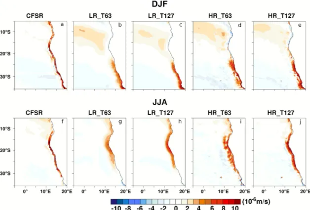
To assess the representation of the Benguela coastal upwelling system, we examine seasonal averages of vertical velocity at a depth of 20 m (Fig. 5). This depth is chosen because upwelling is most intense in the upper meters of the water column. CFSR current velocities indicate that coastal upwelling occurs over a narrow, along-shore band which extends over a variable latitudinal band depending on the season (Fig. 5a, f). In DJF, upwelling is found from 5° S to the south with continuous velocities close to 10 × 10^–6 m/s

Fig. 5 Seasonal means of vertical velocity, in 10–6 m/s, given at a depth of 20 m as computed from CFSR reanalysis (a, f), LR_T63 (b, g), LR_T127 (c, h), HR_T63 (d, i) and HR_T127 (e, j) averaged for

the 1988–2007 period. Positive values point to upwelling and nega- tives ones downwelling. Upper row DJF, lower row JJA

(9)

from about 35° to 23° S. In this season, all our setups fail to represent the intense upwelling near the ABFZ captured in CFSR. In JJA, upwelling develops from 10° to 30° S, with velocities near 10 × 10^–6 m/s from about 15° to 25° S.

Vertical velocities from LR_T63 also exhibit a clear seasonal shift (Fig. 5b, g).In DJF, in line with CFSR, upwelling is particularly intense from 35° to 23° S. In JJA, upwelling occurs from near the equator to 25° S, whilst it extends further south in CFSR. In both seasons, velocities are underestimated and do not attain values typical of CFSR in the near-shore area. Also, upwelling regions extend too far west in comparison to reanalysis data in LR_T63. The increase of the atmospheric resolution in LR_T127 leads to vertical velocities more confined to the coast (Fig. 5c, h). Regardless of the season, vertical velocities in LR_T127 are stronger than in LR_T63.

The higher oceanic resolution in HR_T63 improves the representation of upwelling, which becomes closer to CFSR especially over the regions adjacent to the coast (Fig. 5d, i). Upwelling in HR_T63 is slightly stronger than in both LR configurations and simulated vertical velocities attain values close to ~ 10 × 10^–6 m/s in DJF. In JJA, upwelling regions extend further south. Results presented so far, are in line with Small et al. (2015), who found

that a realistic representation of horizontal currents and upwelling involves small-scale motions which are only captured with a high-resolution oceanic grid. However, positive velocities are not as close to the coast as in LR_

T127, pointing to the impact of atmospheric resolution in the narrowing of the band of coastal upwelling. Again, the most realistic representation is obtained with HR_T127 (Fig. 5e, j). In this case, higher atmospheric resolution brings upwelling areas closer to the coast and higher oceanic resolution strengthens notably coastal along-shore vertical velocities, which become closer in magnitude to those from CFSR.

3.3 Role of model resolution in the representation of atmospheric dynamics

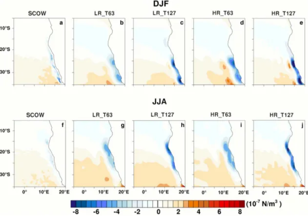
3.3.1 Meridional wind and wind stress curl

Coastal currents and upwelling systems are set to a large extent by the wind distribution near the coast (e.g., Small et al. 2015). The connection between the Benguela upwelling system and wind representation is twofold. On the one hand, strong near-shore wind stress parallel to the coast directed towards the equator leads to westward

Fig. 6 Seasonal averages of meridional wind speed, expressed in m/s, computed from SCOW (a, f), LR_T63 (b, g), LR_T127 (c, h), HR_T63 (d, i) and HR_T127 (e, j) for the 1988–2007 time period. Upper row DJF, lower row JJA

(10)

transport and coastal upwelling (Bakun 1990). On the other hand, negative wind stress curl close to the coast generates Ekman pumping, inducing upwelling (Enriquez and Friehe 1995). In the analysis below, we evaluate the ability of the different model configurations to reproduce the seasonal variability of the meridional wind speed at 10 m (Fig. 6) and the wind stress curl (Fig. 7). Meridional wind speed from SCOW indicates that prevailing winds are equatorward (Fig. 6a, f). In DJF, near-shore wind speeds are 5 m/s or higher from about 15° S to the south. A maximum that exceeds 8 m/s arises near shore, close to 28° S. In JJA, near- shore wind speeds greater than 5 m/s appear from ~ 25°–27°

S northward and, in two small areas between 15° and 20° S, maximum speeds of ~ 7 m/s arise. It is worth noting that the seasonally-dependent location of the areas where maximum wind speeds arise show a good agreement with the position of the most intense upwelling areas (Fig. 5) and the regions where maximum frequencies of occurrence of the Benguela coastal low-level jet are found (Lima et al. 2018a, b). This is to be expected since southerly surface winds associated with the Benguela low-level coastal jet exert a first-order control on the development of the Benguela upwelling system (e.g.

Patricola and Chang 2017). The LR_T63 simulation does not reproduce the maximum velocities found in SCOW in

DJF and shows a rather sharp and unrealistic wind slacken- ing north of 15° S (Fig. 6b). In JJA, a maximum of the same magnitude as in SCOW is simulated, but the area over which it extends is overestimated (Fig. 6g). The refinement of the atmospheric resolution in LR_T127 leads to an improved, smoother meridional wind speed pattern (Fig. 6c, h). How- ever, in DJF, the maximum velocities from SCOW are still not found in LR_T127. In JJA, the surface area over which the maximum speeds occur becomes smaller than with LR_

T63, but this is still larger than in SCOW.

Interestingly, the combination of a coarse atmospheric grid with a refined, eddy-permitting ocean grid in HR_T63 triggers the development of a maximum meridional wind of 8 m/s in DJF (Fig. 6d). Whereas this maximum appears displaced offshore and its surface area is overestimated, this result stresses that a solely increase of the oceanic resolution promotes maximum wind speeds of the correct magnitude.

This could indicate that the decrease of the SST along the Namibian coast with a finer-resolution oceanic grid acceler- ates the Benguela coastal low-level jet. In JJA, the surface area over which winds blow more intensely is again magni- fied (Fig. 6i). Results from HR_T127 show that the refinement of both oceanic and atmospheric grids leads to the most accurate representation of meridional winds (Fig. 6e,

Fig. 7 Seasonal means of wind stress curl, in 10–7 N/m³, derived from SCOW (a, f), as well as from LR_T63 (b, g), LR_T127 (c, h), HR_T63 (d, i) and HR_T127 (e, j) for the 1988–2007 period. Upper row DJF, lower row JJA

(11)

j). The largest improvements occur in DJF, when the highest velocities attain a correct regional distribution and magnitude. In JJA, the meridional wind speed pattern is similar to that obtained with LR_T127.

SCOW wind stress curl (hereafter WSC) shows mostly negative values along the African coast in both seasons (Fig. 7a, f). In DJF, three regions where WSC is particularly enhanced are distinguished: (i) between 20° and 25°

S; (ii) between 25° and 30° S and (iii) near Cape Town. In JJA, negative WSC achieves a smaller magnitude (in abso- lute value) and peaks within two regions: (i) near 15° S and (ii) close to 25° S. The LR_T63 configuration reproduces the approximate location of two (out of three) areas where negative WSC is prominent in DJF, although these are larger and extend further offshore than in SCOW (Fig. 7b). Over these two regions WSC is slightly smaller than in SCOW and shows values close to − 4 × 10^–7 N/m³. In JJA, LR_T63 reproduces the two areas with negative WSC but, again, they extend far too seawards (Fig. 7g). The increase of the atmospheric resolution in LR_T127 improves the representation of WSC (Fig. 7c, h). In DJF and JJA, WSC is more negative, appears more confined towards the coast and peaks at the same areas as in LR_T63 (Fig. 7c, h). In DJF, WSC attains up to − 8 × 10^–7 N/m³, in line with SCOW. In JJA, WSC reaches up to − 8 × 10^–7 N/m³ and − 6 × 10^–7 N/m³ in the northern and southern regions of enhanced WSC, respectively. In HR_T63, the areas with negative WSC roughly coincide with those found in LR_T63 but, in this case, negative WSC is more intense and takes values between those from LR_T63 and LR_T127 (Fig. 7d, i). The increase of the oceanic resolution enhances coastal WSC but, as expected, the intensification is smaller than when only the atmospheric resolution is refined. In DJF, the WSC peaks at

− 7.5 × 10^–7 N/m³ and − 4.5 × 10^–7 N/m³ over the northern and southern regions, respectively. In JJA, a subtle intensification relative to LR_T63 is seen. In HR_T127, patterns of negative WSC very similar to those from LR_T127 are found (Fig. 7e, j). Different to LR_T127, in this case, the two peaks reproduced in each season are more extensive, intense and all of them reach up to − 8 × 10^–7 N/m³. Inter- estingly enough, in DJF, the model reproduces a small, moderate-intensity WSC area near 30° S which is also present in SCOW. While an increase of the oceanic resolution intensifies negative WSC, a refinement of the atmospheric grid drives an intensification of WSC and a confinement of the areas where negative WSC arises towards the coast.

As seen in Sect. 3.2.2, a similar response to changes in the atmospheric and oceanic resolutions have been found for the Benguela upwelling system, underlining the clear link between this and wind representation.

3.3.2 Mean sea‑level pressure and wind biases

Wind speed errors driven by mean sea level pressure (MSLP) biases can lead to deficiencies in the simulation of the South Atlantic Anticyclone (SAA). In turn, a misrepresentation of this structure has been related to a weakening of equatorward winds over the SETA region (e.g., Cabos et al. 2017 and references therein). MSLP and 925 hPa wind speed biases with respect to ERA-Interim, respectively, are depicted in Fig. 8. In DJF, all configurations feature systematic negative MSLP biases over the area occupied by the SAA. In JJA the negative MSLP biases become less negative over the eastern Tropical Atlantic and concentrate along a variable extension of the African coast. These biases are a result of both a shifted and weaker SAA, which is reflected in an incorrect position of the ITCZ, and a biased surface wind over the equator. With LR_T63, negative MSLP anomalies are encountered in both seasons (Fig. 8a, e). In DJF, these are located within a band that extends from near the equator to South Africa and then, until the American coast, and biases reach a maximum of − 4 hPa. In JJA, negative MSLP biases are more modest and do not extend further west than 15° W, reaching a maximum of − 3 hPa. When the atmospheric resolution is increased, interesting differences can be observed in comparison to the previous case (Fig. 8b, f). In DJF, maximum values of − 4 hPa are confined towards a less extensive area. In contrast, in JJA, biases extend from the equator to the south with two peaks of − 3 hPa, one near 0°–15° E and another one between 35° and 45° S.

The increase of the oceanic resolution in HR_T63 lowers negative biases substantially (Fig. 8c, g). This indicates that insufficient resolution of the ocean component is an important driver of MSLP biases in coupled models. Although biases in DJF present a similar structure as with the two former configurations, these are generally not larger than

− 2 hPa. In JJA, biases generally do not exceed − 2 hPa and concentrate between 0° and 15° S. An increase of the atmospheric resolution in HR_T127 features small differences relative to HR_T63 (Fig. 8d, h). In DJF, negative MSLP anomalies are not larger than − 2 hPa and concentrate over a slightly stretched latitudinal band relative to HR_T63. The bias distribution found in JJA does not show noticeable differences in comparison to HR_T63 over the SETA. There- fore, improvements in the representation of the MSLP as the model resolution is refined, have a concomitant effect on bias reduction when compared to ERA-Interim. This improves the simulation of the SAA, which reinforces along- shore equatorward winds over the SETA (Fig. 8c, d, g, h).

3.3.3 Net downward heat flux

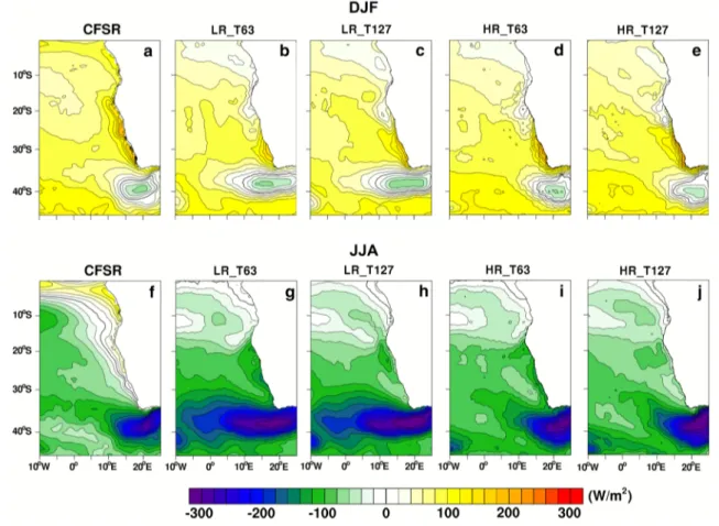
We now explore the seasonal variability of the net heat flux for the different setups, taking as a reference the CFSR

(12)

Fig. 8 Seasonal mean biases of MSLP in hPa (colours) and wind speed in m/s (vectors) for LR_T63 (a, e), LR_T127 (b, f), HR_T63 (c, g) and HR_T127 (d, h) relative to ERA-Interim, averaged over the 1988–2007 time period. Left column DJF, right column JJA

(13)

fluxes (Fig. 9). CFSR indicates that in DJF the strongest positive values arise from about 20° to 35° S near the western coast of Africa, reaching ~ 200 W/m², while the strongest negative flux of about − 80 W/m² is attained where the AgC retroflects (Fig. 9a). In JJA, the heat flux becomes smaller towards the south and maximum negative values within the AgC region reach − 300 W/m² (Fig. 9f). In agreement with CFSR, the net heat flux in LR_T63 is positive over the SETA in DJF (Fig. 9b). Maximum values close to 200 W/m² can be found there, but these are confined too far south. Within the AgC region, as in CFSR, − 80 W/m² are reached. In JJA, the simulated net heat flux is mostly negative along the coast and therefore, smaller than in CFSR (Fig. 9g). As in CFSR, the heat flux becomes more negative to the south and more positive to the north. Close to the AgC, the simulated flux is near − 300 W/m². Focusing on LR_T127, the regional distribution of the heat flux in DJF does not deviate much from that found for LR_T63 (Fig. 9c). However, now positive coastal values greater than with LR_T63 arise from 25° to 35° S, thus improving the heat flux representation (Fig. 9c).

In JJA, the main difference relative to LR_T63 is that, with this configuration, values near the southern portion of the western African coast become less negative (Fig. 9h).

In DJF, with HR_T63, the regional distribution of the heat flux resembles that from LR_T127, but several improvements are noticed (Fig. 9d). First, values greater than 160 W/

m² extend further offshore. Second, the improved simulation of the AgC keeps negative values more confined to the east. In JJA, the simulated heat flux is similar to that derived from LR_T63, but negative near-shore values are in this case less negative from about 20° S along the western coast of Africa (Fig. 9i). The representation of the heat flux within the region occupied by the AgC also improves. The heat flux reproduced with HR_T127 exhibits a similar distribution as in HR_T63 (Fig. 9e, j). The most noticeable differences between HR_T127 and HR_T63 are the increase of the heat flux along the western African coast towards offshore in DJF and the magnitude reduction of negative coastal values from 20° S to the south in JJA. Therefore, the regional distribution of the heat flux improves as the resolution of the model’s components is increased. In DJF, improvements in the simulation of the heat flux are primarily controlled by an enhanced oceanic resolution. In JJA, the heat flux is better reproduced along the southwestern coast of Africa when the atmospheric resolution is high, but this is only properly simulated over the AgC region when also the oceanic grid

Fig. 9 Seasonal averages of the net heat flux, in W/m², computed from CFSR (a, f), LR_T63 (b, g), LR_T127 (c, h), HR_T63 (d, i) and HR_

T127 (e, j) for the 1988–2007 period. A positive sign indicates that the ocean gains heat from the atmosphere. Upper row DJF, lower row JJA

(14)

is refined. It is interesting to point out that, in both seasons, an improved representation of the coastal heat flux entails an increase of its magnitude from 20° S southwards, coinciding with the areas where coastal biases are alleviated (see Fig. 3). This may indicate that warm biases are not linked to an inadequate regional distribution of the heat flux, but rather to the heat supplied through coastal upwelling.

4 Discussion

Our sensitivity study highlights that, although important improvements from LR_T63 to HR_T127 are observed, SST biases remain. Whilst the magnitude of the biases is in line with previous modelling studies (e.g., Toniazzo and Woolnough 2014), the persistence of errors reveals that some dynamical processes and air-sea feedbacks are still not properly simulated. The objective of this section is twofold. On the one hand, we aim to gain physics-based insight into the different mechanisms that drive the improvements observed in the regional distribution of the SST as the model resolution is increased. On the other hand, we try to detect deficiencies in the representation of processes which can potentially contribute to the generation of warm biases over the SETA. Table 2 offers a summary of the mean biases in SST, meridional 10-m wind speed and vertical velocity south of the ABFZ.

4.1 Horizontal heat advection and overshooting of the Angola Current

From the results presented so far one can conclude that in our experiments warm SST biases in the SETA region are primarily alleviated by an increase of the oceanic resolution, whereas changes in the atmospheric resolution seem to be less important. A long-lasting problem common to most models participating in the CMIP5 initiative is the inaccu- rate representation of the AC and the BC (Xu et al. 2014;

Koseki et al. 2018). Generally, the AC is too strong and/or the BC is too weak, giving place to an overshooting of the AC which in turn provokes a southward shift of the ABFZ in comparison to observations. The wrong configuration of these currents has been linked to unrealistic heat advection to high southern latitudes that contributes to overheating of the SETA region (Xu et al. 2014). The seasonal cycle of the latitudinal position of the ABFZ, defined by the maximum meridional SST gradient (see Colberg and Reason 2006), is illustrated in Fig. 10. For the time period considered, in agreement with Lass et al. (2010), CFSR shows that the ABFZ is near 16° S and is subjected to a subtle latitudinal variation over the year (Fig. 10a). The ABFZ is well defined in all months except from June to September, when its position is more diffuse (Meeuwis and Lutjeharms 1990).

Although in the simulated results the ABFZ is visible, this is not as clearly depicted as in CFSR (Fig. 10b–e). In all setups, the ABFZ appears to be displaced to the south in austral winter and summer. This is not in agreement with results from Cabos et al. (2017), which indicate that the overshooting of the AC is a typical feature of DJF. The southward shift of the ABFZ is more pronounced with LR_T63 and more modest with HR_T127. Specifically, with LR_T63, the front is placed near 26° S in DJF and close to 29° S in JJA. With HR_T127, this is found near 23°–24° S in DJF and at about 23° S in JJA. The values we report are close to 25° S, which nearly coincides with the converge zone derived from the CMIP5 multi-model ensemble mean (Xu et al. 2014). In Fig. 10 we also observe that the position of the front is also consistent with enhanced upwelling, which has been found to be one of the sources of frontogenesis (Koseki et al. 2019). The intensification of upwelling with the HR configurations (refined oceanic resolution), specially with HR_T127, can also be appreciated from this figure.

The southward migration of the ABFZ, set by the relative importance of the near-surface (opposing) Angola and Benguela currents, has a clear imprint on the horizontal heat transport and therefore on water temperature, which are both computed at a depth of 10 m (Fig. 11). Regard- less of the season, the increase of the oceanic resolution (HR) narrows the AC, which is closer to the coast and this reduces offshore biases (see Fig. 3). To the south, water temperature lowers remarkably when the oceanic resolution is enhanced. The increased transport of colder waters in this region with HR is caused by (i) an intensification of the BC and (ii) the development of a series of energetic rings associated with the AgC that transport cold waters towards the northwest (see also Fig. 4). Our results thus corroborate that the southward displacement of the ABFZ is translated into an excessive heat transport via the AC which occurs in all seasons and is more exacerbated when the oceanic resolution is low (see also Zuidema et al. 2016). The main conclusion from the results described in Sect. 3.1 is that,

Table 2 Biases in the simulated mean sea-surface temperature (°C), meridional 10-m wind speed (m/s) and vertical velocity at a depth of 20 m (10–6 m/s) for the different model configurations

Calculations are performed over the ABA2 region (defined in Sect. 4.2), taking into account the 1988–2007 period. Biases in sea- surface temperature are computed with respect to OISSTV2. Wind biases are calculated relative to SCOW. Biases in vertical velocity are expressed with respect to CFSR. Positive biases indicate that the corresponding variables are overestimated

LR_T63 LR_T127 HR_T63 HR_T127 Sea-surface temperature 7.55 6.32 6.26 4.41 Meridional 10-m wind

speed − 1.18 − 0.91 − 0.55 − 0.28

Vertical ocean velocity − 2.28 − 1.92 − 0.60 − 0.60

(15)

regardless of the season, SST biases are particularly reduced when the oceanic resolution is refined, i.e., in HR_T63 and HR_T127 (Fig. 3). Specifically, the sharpest SST decrease takes place approximately over the region occupied by the BC in our simulations. This indicates that strengthening of the BC, which only occurs with a refined ocean resolution (Fig. 4), is contributing importantly to the alleviation of SST biases. Overall, the intensity of the geostrophically adjusted, equatorward BC is set by: (i) the Agulhas leakage, (ii) surface southerly winds blowing along the Angolan-Namibian coasts and (iii) bathymetric features. Previous works have shown that the AgC provides momentum to the BC by means of the Agulhas leakage (Veitch and Penven 2017).

We propose that the improved simulation of the AgC and its associated rings, which is only achieved when the resolution of the oceanic component is high, provides kinetic energy to the BC. This, in turn, favours its correct representation in terms of trajectory and intensity. In addition to that, these rings transport cold water from the south towards the northwest, therefore contributing to a reduction of offshore warm biases (see Figs. 3 and 11).

As to the role of winds, in Sect. 3.3.1 we find that, with a coarse oceanic grid, the increase of the atmospheric resolution from T63 to T127 improves to a large extent the representation of southerly meridional winds (Fig. 6). However, with LR_T127 the BC is still too weak and, as stated above, a significant reinforcement of this current requires a high- resolution oceanic grid. This suggests that improvements observed in the representation of the BC may be attributed to the refined resolution of the oceanic component. A key insight extracted from Sect. 3.2.1 is that, even with a high- resolution oceanic grid, a cyclonic structure that limits the northward path of the BC arises when the atmospheric resolution is coarse (Fig. 4). This cyclonic structure is more developed with HR_T63 and is nearly vanished with HR_

T127. The origin of this cyclonic error may be related to the observed offshore displacement of the areas where southerly winds are maximum when atmospheric resolution is coarse, which may cause negative near-shore wind stress curl to extend further offshore (Fig. 7). The seaward shift of wind maximum over this region with a low-resolution atmospheric grid has also been encountered in previous works

Fig. 10 Seasonal cycle of the meridional gradient of SST (°C/105 m;

colours) averaged over 11°–14° E to 10°–32° S, as well as the vertical velocity at a depth of 20 m (10–6 m/s; contours). These are com-

puted from CFSR (a), LR_T63 (b), LR_T127 (c), HR_T63 (d) and HR_T127 (e), for the 1988–2007 time period

(16)

(e.g., Patricola et al. 2016). Within this area, wind stress curl provides negative vorticity, consistent with cyclonic motion in the southern hemisphere. The impact of bathymetric features on the near-surface configuration will be tackled in Sect. 4.4 of the discussion.

4.2 Sensitivity to coastal upwelling: vertical velocities vs thermocline

Xu et al. (2014) find that the intensity of coastal upwelling, given as the vertical mass transport, is not directly corre- lated to the severity of SST biases over the SETA. This, they argue, implies that vertical heat advection is not exerting a primary control on the development of coastal overheating.

In contrast to this, our results show that the regions where SST biases are reduced from LR_T63 to HR_T127, roughly coincide with locations where upwelling is enhanced (Figs. 3 and 5). This is an indication that in our experiments upwelling is a contributing factor to the bias generation. As seen in Sect. 3.2.2, coastal upwelling is more intense and closer to the coast when the atmospheric resolution is finer, whereas a solely refinement of the oceanic grid leads to a more pronounced strengthening of the upwelling system (Fig. 5). The confinement of upwelling to the near-shore

region is intimately related to the WSC which, in line with the findings of Patricola et al. (2016), becomes negative over a narrower, along-shore band when the atmospheric resolution is finer (Fig. 7). The enhanced upwelling with a higher-resolution oceanic grid may be set by the intensification of the BC due to the reasons described above. Although with HR_T127 upwelling has a similar magnitude and a similar regional distribution relative to CFSR along most of the Namibian coast, especially in DJF, warm biases still remain over this region. This allows us to conclude that, in HR_T127, insufficient upwelling is not the major driver of SST biases. Our results rather point to deficiencies in the representation of the sharp thermocline of the SETA, caus- ing an uplift of waters which are warmer than observations (Richter 2015; Cabos et al. 2017). This is supported by Fig.

S2 of the Supplementary Material, which shows that warm biases extend from the surface over the water column in the region occupied by the BC, especially when the model resolution is coarse (LR_T63). In addition to this, our results allow us to discard vertical stratification of the water column as a primary driver of insufficient upwelling in LR (see Fig.

S3).To assess this aspect, we examine the seasonal cycle of water temperature averaged over the box areas 9.5°–15° E,

Fig. 11 Seasonal averages of water temperature in °C (colours) and horizontal heat transport in K·m/s (u·T; vectors) both at a depth of 10 m. These are computed from CFSR (a, f), LR_T63 (b, g), LR_

T127 (c, h), HR_T63 (d, i) and HR_T127 (e, j) for the 1988–2007 period. Upper row DJF, lower row JJA

(17)

21°–15.5° S (thereafter ABA1) and 12.5°–16° E, 27.5°–21°

S (thereafter ABA2) depicted in Fig. 1, evaluated at a depth of 40 m (Fig. 12). This depth is chosen because, in our experiments, vertical velocity (i.e., upwelling) is strongest in the upper meters of the water column (see Fig. S2 of the Supplementary Material). Whilst in the work of Castaño- Tierno et al. (2018) the thermocline is defined as the depth of maximum vertical thermal gradient, we consider that the study of water temperature at the depth of maximum upwelling is a good first-order approximation to evaluate the modelled subsurface water temperature relative to CFSR.

ABA1 includes the ABFZ and is similar to the ABA (Angola Benguela Area) region used in Lübbecke et al. (2010). It covers the zone of ABA in which our refined setups show improvements with respect to ocean temperature biases. The ABA2 region includes part of the northern domain of the Benguela upwelling system, where the refinement of the grids leads to the strongest improvements in the simulated SST. Throughout the year, in both ABA1 (Fig. 12a) and ABA2 (Fig. 12b) regions, the model simulations produce higher temperatures than observations. In particular, the better and worst agreement with observations is obtained with HR_T127 and LR_T63, respectively. This is consistent with the fact that the average heat content at ABA1 and ABA2 at shallow depths (150 m and 300 m), takes the maximum and minimum values with LR_T63 and HR_T127, respectively, and that heat content is more importantly reduced when the oceanic resolution increases (not shown). These findings support the hypothesis that upwelled waters warmer than observations are contributing to warm biases. As expected, HR_T127 and LR_T63 show better and worst agreement with observations, respectively, with ABA2 being the region that shows a more noticeable improvement with HR_T127 relative to LR_T63. The temperature drop observed as the model resolution increases, especially with HR_T127, is in line with the reduction of biases observed with those

configurations (see Fig. 3). The fact that temperature differences with CFSR are larger in JJA than in DJF, is consistent with a less pronounced bias reduction in JJA, partly due to the underestimation of the intensity of the BC (see Sect. 3.1).

At this point, it is interesting to investigate the mechanisms that cause the misrepresentation of sub-surface water temperature. A well-known feature of the Tropical Atlantic basin is the presence of a strong zonal temperature gradient caused by cold waters along its eastern rim and warmer waters along its western flank. According to Seager et al.

(2003), this temperature gradient is sustained by oceanic processes, namely water transport. Water transport promotes dynamic upwelling and cools down surface waters which are subsequently horizontally advected. The SAA reinforces coastal upwelling and favours equatorward advection of cold waters over the eastern Atlantic, while it intensifies pole- ward flow of warm temperatures over the western Atlantic.

Therefore, insufficient northward transport due to a weakening of the BC will lead to a reduced east–west temperature gradient and to a deficient representation of the SAA due to subsidence reduction in the eastern part of the basin and convection in the western coast of the midlatitude ocean.

This mechanism could also induce temperature biases in other regions of the basin via horizontal advection through near-surface currents.

The SST anomalies relative to the zonal mean are presented in Fig. 13. OISSTV2 shows that, in line with Seager et al. (2003), negative zonal anomalies arise to the east, while positive anomalies concentrate to the west of the Trop- ical Atlantic (Fig. 13a, f). In spite of quantitative differences, the simulated zonal anomalies of SST exhibit spatial patterns similar to OISSTV2 in DJF (Fig. 13b–e). Specifically, when the atmospheric resolution is low, zonal anomalies of SST are smaller than in IOSSTV2. Zonal temperature anomalies are better represented when the oceanic resolution

Fig. 12 Monthly-average cycle of water temperature at 40 m, expressed in °C, averaged over ABA1 (a) and ABA2 (b), as defined in Sect. 4.2, for the 1988–2007 period (CFSR:

brown; LR_T63: blue dots;

LR_T127: blue, dashed line;

HR_T63: red dots; HR_T127:

red, dashed line; LR_UNC:

blue; HR_UNC: red). Note that the last two configurations (UNC) will be described in Sect. 4.4

(18)

Fig. 13 Seasonal averages of SST anomalies relative to the zonal mean computed for each latitude, in °C, from OISSTV2 (a, f), LR_T63 (b, g), LR_T127 (c, h), HR_T63 (d, i) and HR_T127 (e, j) over the 1988–2007 time period. Left column DJF, right column JJA

(19)

increases, thus supporting the idea that this thermal asym- metry is primarily controlled by oceanic processes. In JJA, the model has more difficulties to reproduce the pattern inferred from OISSTV2 (Fig. 13g–j). In view of our results, the mechanism proposed by Seager et al. (2003) seems to play a relevant role in the generation of biases over the SETA. According to our findings, overheating of the water column would be induced by a weakening of the BC, which does not advect enough cold waters to the north, reducing the SST gradient between the eastern and western rims of the South Atlantic. In that case, air-sea feedbacks decrease the intensity of the SAA (see Fig. 8), reducing even more the northward transport of low-temperature waters due to a weakening of equatorward winds over the eastern Atlan- tic. This would finally lead to upwelling of waters with an anomalously high temperature.

4.3 Role of the atmospheric heat flux components Results presented in Sect. 3.3.3 indicate that the regional distribution of the net heat flux is better reproduced as

the model resolution is refined, especially in DJF. In both seasons, improvements involve an alongshore increase of the net heat flux from about 20° S all the way to the south, roughly coinciding with the areas where biases become smaller. Whereas this is a first-order indication that the heat flux is not a key player in the generation of coastal SST biases, it is still interesting to examine the individual contri- butions of the different components of the heat flux. In this context, a well-known drawback of atmospheric models is their inability to reproduce realistically the low-level strato- cumulus clouds over the eastern subtropical oceans (Richter and Mechoso 2006). The underestimation of the cloud cover, in turn, has been associated to an unrealistic warming of the sea surface due to an excessive penetration of solar radiation over the SETA (Huang et al. 2007; Wahl et al. 2011).

Figure 14 shows that, in DJF, near-shore incoming radiation from about 20° S southward becomes generally smaller as the atmospheric and oceanic resolutions are refined. In JJA, differences between the different setups from 20° S to the south are relatively small. These results provide evidence that the observed increase of the heat flux over the SETA is

Fig. 14 Seasonal averages of incoming surface shortwave radiation, in W/m², computed from SARAH (a, f), LR_T63 (b, g), LR_T127 (c, h), HR_T63 (d, i) and HR_T127 (e, j) for the 1988–2007. Upper row DJF, lower row JJA

(20)

Fig. 15 Monthly-average cycle of the downward shortwave flux (a, b), net longwave flux (c, d), sensible (e, f) and latent heat fluxes (g, h), in W/m², within ABA1 and ABA2 regions, as defined in Sect. 4.2, for the 1988–2007 period (CFSR:

brown; OAFlux: black; LR_

T63: blue dots; LR_T127: blue, dashed line; HR_T63: red dots;

HR_T127: red, dashed line)

(21)

not driven by an increase of the incoming radiation, mean- ing that a correct representation of low-level deck clouds alone is insufficient to improve simulated biases in our experiments. The seasonal cycle of the incoming shortwave radiation is well captured in ABA1 and ABA2 (Fig. 15a, b).

Simulated curves take intermediate values between CFSR and OAFlux. Setups with higher atmospheric resolution are closer to OAFlux.

Similarly to the shortwave radiation, the seasonal variability of the net longwave radiation appears relatively well captured within ABA1 and ABA2 (Fig. 15c, d). Curves constructed from LR_T127 and HR_T127 closely match observations. On the other side, longwave radiation from coarser atmospheric configurations is slightly lower than observations, especially in JJA. The computed sensible heat flux exhibits lower values than observations (Fig. 15e, f).

Simulated curves present a stronger seasonal amplitude than observations, but it is difficult to qualitatively determine whether the seasonal cycle is well captured or not due to the differences in the data from OAFlux and CFSR. Values from the simulated curves and the datasets deviate more in JJA, when the differences can be as large as 50 W/m². Whereas the sensible heat flux may contribute to the negative heat flux biases in JJA, this component cannot fully explain the observed differences relative to CFSR in the coastal regions with LR_T63 (see Fig. 9f, g). The seasonal cycle of the latent heat flux shows the largest differences in comparison to OAFlux and CFSR curves (Fig. 15g, h). The simulated seasonal cycles are up to about 100 W/m² more negative than in the datasets in the central months of the year. Differ- ences are minimised in T127. In view of our results, we can conclude that the negative heat flux biases encountered in JJA relative to CFSR (Fig. 9) are triggered by an excessive latent heat loss and exacerbated by a too negative sensible heat flux. In JJA, when warm biases are the largest, enhanced warming of surface waters increases evaporation and leads to an excessive heat loss via the latent heat flux. In DJF, when warm biases are more modest, latent heat losses are less pronounced (see e.g., Xu et al. 2014; Cabos et al. 2017).

4.4 Coupled vs uncoupled simulations: role of air‑sea feedbacks in SST biases

To qualitatively assess the role of air–sea coupling in the occurrence of coastal SST biases over the SETA, two com- plementary uncoupled simulations have been run. The FESOM configurations in these simulations are identical to the ones used in the coupled simulations (LR and HR). As observed in Fig. 16a, b, annual-mean SST biases from LR_

UNC and HR_UNC are much smaller than those derived from any of the coupled configurations (see Figs. 2 and 3).

Specifically, from about 15° S to the south, coastal biases do not exceed 2 °C with LR_UNC and 1 °C with HR_UNC,

these being as large as 6 °C with LR_T63. In the Supple- mentary Material (Fig. S4a, b) we show that within ABA1 and ABA2, the seasonal cycle of the net heat flux with HR_

UNC is close to the curves derived from the datasets. In comparison to the coupled runs, the net heat flux reproduced in the stand-alone simulations increases, especially in the central months of the year.

To determine the impact of the improved representation of atmospheric fluxes on the ocean circulation we examine zonal anomalies of SST for LR_UNC and HR_UNC (Fig. 16c–f). The forced runs show a far better simulation of the SST gradient than any of the coupled configurations.

This is particularly clear with HR_UNC, where the negative values of zonal SST anomalies along the African coast attain a higher magnitude and a better representation of the zonal SST gradients is achieved. This in turn drives an improved simulation of ocean temperature at a depth of 40 m within ABA1 and ABA2, especially in HR_UNC (Fig. 12). In Sect. 4.1 we stated that a more detailed bathymetry could lead to a better simulation of ocean currents. The fact that both LR_UNC and HR_UNC exhibit smaller coastal SST biases than in any of the coupled configurations indicates that bathymetric features are not the main drivers of the misrepresentation of ocean currents when the oceanic resolution is low. Therefore, the coupling strongly changes the simulated SST and, as a consequence, a less realistic heat flux develops in the coupled runs. This, in turn, influences both the atmospheric and oceanic circulations within the SETA region, magnifying the ocean biases. The effect of the coupling is modulated by both the atmospheric and oceanic resolutions. The impact of atmospheric resolution can be seen in changes of the wind stress curl spatial distribution and strength when we change atmospheric resolution keeping the same ocean resolution (i.e., compare LR_T63 and LR_T127 or HR_T63 and HR_T127). Wind changes impact atmospheric fluxes and, to a lesser extent, both the coastal circulation and the Agulhas current. The increase of the ocean resolution from the coarse LR to the locally eddy-permitting HR setup leads to a better simulation of the boundary currents, upwelling and SST gradients (see Figs. 13 and 16, where the zonal SST anomalies for coupled and uncoupled runs are represented). These changes have a concomitant effect on the simulated wind. In turn, these regional changes influence the atmospheric and oceanic large-scale circulation over the South Atlantic. This is reflected in the strength and location of the South Atlantic anticyclone and the SST zonal anomalies distribution. We can infer that the regional-scale feedbacks in the SETA region determine the upwelling, the wind strength and atmospheric fluxes in the region, which are not only important locally, but also influence the basin- wide circulation. Consequently, the large-scale atmospheric and oceanic circulations (through the subsurface circulation and SAA strength and location) have a large impact

(22)

on the SETA simulated SST. Although out of the scope of this work, it is interesting to note that an additional analysis performed (not shown) reveals that an increase of the atmospheric and oceanic model resolution is beneficial to improve the Bjerknes Feedback in the equatorial Atlantic

(e.g., Keenlyside and Latif 2007) and possibly in the coastal upwelling region (coastal Bjerknes Feedback, Kataoka et al.

2013). A more extensive analysis addressing the role of the oceanic and atmospheric resolutions in the Bjerkness Feed- back could constitute an excellent follow-up of this work.

Fig. 16 Annual-mean SST bias relative to HadISST climatology for LR_UNC (a) and HR_UNC (b), in °C. Seasonal averages of SST anomalies relative to the zonal mean calculated for each latitude, in

°C, for LR_UNC (c, e) and HR_UNC (d, f). Means are computed for the 1988–2007 period