The influence of dissolved organic matter on the marine production of carbonyl sulfide (OCS) and carbon disulfide (CS
2) in the Eastern Tropical South Pacific
Sinikka T. Lennartz
1,a, Marc von Hobe
2, Dennis Booge
1, Henry Bittig
3, Tim Fischer
1, Rafael
5
Gonçalves-Araujo
4,5, Kerstin B. Ksionzek
4,6, Boris P. Koch
4,7,8, Astrid Bracher
4,8, Rüdiger Röttgers
9, Birgit Quack
1, Christa A. Marandino
11 GEOMAR Helmholtz Centre for Ocean Research Kiel, Düsternbrooker Weg 20, 24105 Kiel, Germany
2 Forschungszentrum Jülich GmbH, Institute of Energy and Climate Research (IEK-7), Wilhelm-Johnen-Strasse, 52425 10 Jülich, Germany
3 Leibniz Institute for Baltic Sea Research Warnemünde, Seestraße 15, D-18119 Rostock
4 Alfred Wegener Institute Helmholtz Centre for Polar and Marine Research, Am Handelshafen 12, 27570 Bremerhaven, Germany
5Aarhus University, Department of Bioscience, Frederiksborgvej 399, 4000 Roskilde, Denmark 15 6MARUM Center for Marine Environmental Sciences, Leobener Straße, D-28359 Bremen, Germany.
7 University of Applied Sciences, An der Karlstadt, 27568 Bremerhaven
8 Institute of Environmental Physics, University of Bremen, 28334 Bremen, Germany
9 Helmholtz-Zentrum Geesthacht, 21502 Geesthacht, Germany
anow at: Insitute for Biology and Chemistry of the Marine Environment, University of Oldenburg, Oldenburg 20
Correspondence to: Sinikka T. Lennartz (sinikka.lennartz@uni-oldenburg.com)
Abstract. Oceanic emissions of the climate relevant trace gases carbonyl sulfide (OCS) and carbon disulfide (CS2) are a major source to their atmospheric budget. Their current and future emission estimates are still uncertain due to incomplete process understanding and, therefore, inexact quantification across different biogeochemical regimes. Here we present the 25
first concurrent measurements of both gases together with related fractions of the dissolved organic matter (DOM) pool, i.e.
solid-phase extractable dissolved organic sulfur (DOSSPE), chromophoric (CDOM) and fluorescent dissolved organic matter (FDOM) from the Eastern Tropical South Pacific (ETSP). These observations are used to estimate in-situ production rates and identify their drivers. We find different limiting factors of marine photoproduction: while OCS production is limited by the humic-like DOM fraction that can act as a photosensitizer, high CS2 production coincides with high DOSSPE 30
concentration. The lack of correlation between OCS production and DOSSPE may be explained by the active cycling of sulfur between OCS and dissolved inorganic sulfide via OCS photoproduction and hydrolysis. In addition, the only existing parameterization for OCS dark production is validated and updated with new rates from the ETSP and the Indian Ocean. Our results will help to predict oceanic concentrations and emissions of both gases on regional and, potentially, global scales.
35
1
1 Introduction
Oceanic emissions play a dominant role in the atmospheric budget of the climate relevant trace gases carbonyl sulfide (OCS) and carbon disulfide (CS2) (Chin and Davis, 1993; Kremser et al., 2016). OCS is the most abundant sulfur gas in the atmosphere, and CS2 is its most important precursor. Both gases influence the climate directly (OCS) or indirectly (CS2 by oxidation to OCS in the atmosphere), as OCS is a major supplier of stratospheric aerosols (Brühl et al., 2012; Crutzen, 5
1976), which exert a cooling effect on the atmosphere and can foster ozone depletion (Junge et al., 1961; Kremser et al., 2016). Furthermore, OCS has been suggested as a proxy to constrain global terrestrial gross primary production (Campbell et al., 2008; Montzka et al., 2007; Berry et al., 2013). The oceanic emissions of both gases have recently gained interest because they are suggested to account for a missing source of atmospheric OCS (Berry et al., 2013; Kuai et al., 2015;
Glatthor et al., 2015; Launois et al., 2015). In-situ measurements of OCS in surface seawater are still limited, but those 10
available suggest that oceanic emissions are too low to fill the proposed gap of 400-600 Gg S yr-1 in the atmospheric budget (Lennartz et al., 2017). Still, oceanic emission estimates are associated with high uncertainties (ca. 50%) (Kremser et al., 2016; Whelan et al., 2018). Reducing these uncertainties for present and future emission estimates requires i) increasing the existing field data across various biogeochemical regimes and ii) increasing process understanding and quantification in the whole water column to facilitate model approaches.
15
Most of the in-situ observations of OCS and CS2 in seawater were reported from the Atlantic Ocean and adjacent seas, and mainly represent surface ocean measurements (see Whelan et al. (2018) for an overview). Here we report the first concurrent measurements in the surface ocean and the water column for both gases from the Eastern Tropical South Pacific (ETSP). The ETSP is one of the most biologically productive regions in the global ocean, due to the upwelling of nutrient rich water. The upwelling influences the pool of dissolved organic matter (DOM) exposed to sunlight by transporting DOM from the deep 20
ocean to the surface. The DOM pool is relevant in this context, because it contains the precursors and photosensitizers for the photochemical production of OCS and CS2 (Pos et al., 1998; Flöck et al., 1997; Uher and Andreae, 1997). Here we show measurements of chromophoric and fluorescent DOM as well as solid-phase extractable dissolved organic sulfur (DOSSPE), in order to further specify drivers of production processes and improve parameterizations of production rates in biogeochemical models.
25
Chromophoric DOM (CDOM) is the fraction that absorbs light in the UV and visible range, and contains the photosensitizers that absorb light and form radicals for photochemical reactions (Coble, 2007). A part of the CDOM fraction fluoresces (FDOM), i.e. emits absorbed light at a shifted wavelength. Distinct groups of molecules have a specific fluorescence pattern, enabling the molecule classes such as humic substances or proteins (FDOM components) to be differentiated (Coble, 2007; Murphy et al., 2013). DOSSPE is operationally defined as the dissolved organic sulfur retained by 30
solid-phase extraction (Dittmar et al., 2008). The method favors the retention of polar molecules, which comprise approximately 40 % of the total dissolved organic carbon (DOC) in marine waters. Due to the operational definition, no direct comparison to the CDOM and FDOM pools is possible (Wünsch et al., 2018).
2
OCS is produced in the surface ocean by interaction of UV radiation with CDOM (Uher and Andreae, 1997). A reaction pathway through an acylradical intermediate in addition to a thiyl (organic RS·) or sulfhydryl (inorganic SH·, from bisulfide) radical pathway has been proposed by Pos et al. (1998) based on incubation experiments. Indeed, the amount of OCS produced has been shown to depend on CDOM and a variety of organic sulfur-containing precursors, such as methionine or gluthathione (Zepp and Andreae, 1994; Flöck et al., 1997). On larger spatial scales, the CDOM absorption coefficient at 350 5
nm (a350) can serve as a proxy for both photoexcitable carbonyl-groups and organic sulfur precursors, making the overall photoproduction rate second-order dependent on a350 (von Hobe et al., 2003). Accordingly, a global parameterization for photochemical production was developed based on a350, by integrating data from the Atlantic, Pacific and Indian ocean (Lennartz et al., 2017). To improve this parameterization on a regional scale, we tested whether the precursors can be further specified by an easily measurable fraction of the DOM pool (FDOM components, DOSSPE), without performing costly and 10
potentially incomplete analysis on the molecular level. In addition, OCS is produced in a light-independent reaction termed dark production (Flöck and Andreae, 1996; Von Hobe et al., 2001). Two hypotheses exist to date: an abiotic reaction involving thiyl radicals formed by O2 or metal complexes (Pos et al., 1998; Flöck et al., 1997; Flöck and Andreae, 1996), and a coupling to microbial processes during organic matter remineralization (Radford-Knȩry and Cutter, 1994). Dark production is parameterized based on temperature and a350 derived from field data in the Atlantic Ocean and the 15
Mediterranean Sea (Von Hobe et al., 2001). It is yet unclear whether this parameterization is valid on a global scale.
Furthermore, OCS is degraded by hydrolysis yielding CO2 and hydrogen sulfide (H2S) or bisulfide (SH-), in the following summarized as sulfide. The hydrolysis degradation rate increases strongly with temperature, and has been well quantified by a comprehensive laboratory study over a wide temperature range (Elliott et al., 1989) and by seawater incubation studies (Radford-Knȩry and Cutter, 1994). Oceanic OCS concentrations have been modelled using surface box models on regional 20
(von Hobe et al., 2003) and global scales (Lennartz et al., 2017), in the water column (von Hobe et al., 2003) as well as with a global 3D circulation model (Launois et al., 2015) based on the parameterizations above. Here we test whether subsurface concentrations can be numerically simulated by coupling the box model to a physical 1D water column host model.
Production and loss processes for CS2 are less well constrained. Photochemical incubation studies indicate that the photoproduction of CS2 has a similar wavelength-dependence (spectrally resolved apparent quantum yield, AQY), but only a 25
quarter of the magnitude compared to OCS (Xie et al., 1998). It is currently unclear whether in-situ photoproduction rates of both gases co-vary on larger spatial scales. A covariation is expected only when identical drivers limit the production for both gases. Evidence for biological production comes from incubation studies (Xie et al., 1999), indicating varying CS2
production for different phytoplankton species. Outgassing to the atmosphere appears to be the most important sink for CS2
in the mixed layer (Kettle, 2000). Although CS2 is hydrolyzed and oxidized by H2O2, the corresponding lifetimes are too 30
long to rival emission to the atmosphere at the surface (Elliott, 1990). Additional to this long lifetime due to hydrolysis and oxidation, Kettle (2000) proposed a sink with a lifetime on the order of weeks, to match observed concentrations with a surface box model. No underlying mechanism for such a sink is currently known, hampering further model approaches.
3
The goal of this study is to quantify production rates for both gases in the ETSP and to further specify their drivers. We use the comprehensive dataset together with simple biogeochemical models to increase the understanding and quantification of the cycling of both gases in the water column and to improve model capability to predict OCS and CS2 seawater concentrations.
2 Material and Methods 5
2.1 Study area
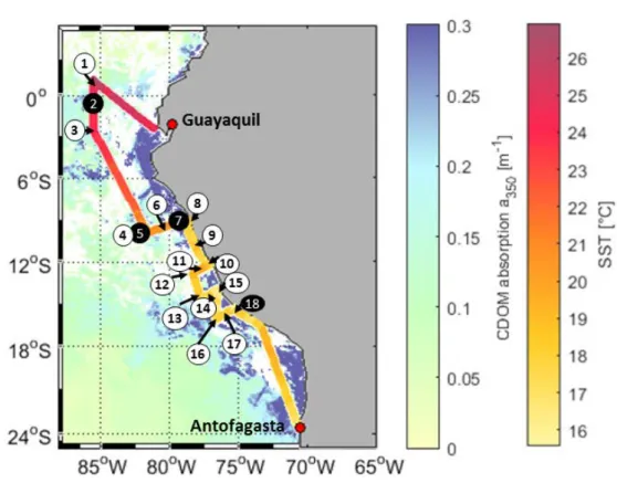
The cruise ASTRA-OMZ on RV SONNE started in Guayaquil, Ecuador, on 05.10.2015 and reached Antofagasta on 22.10.2015 (Fig. 1). It covered several regimes from the open ocean to the coastal shelf between 5°N and 17°S. The hydrographic conditions encountered during this cruise have been described elsewhere (Stramma et al., 2016). The area off Peru belongs to one of the four major global eastern boundary upwelling systems (Chavez et al., 2008). A large oxygen 10
minimum zone expands into the Pacific Ocean at depths between 100 and 900 m, resulting from weak ventilation and strong respiration (Karstensen et al., 2008). The cruise covered areas of open ocean with warm sea surface temperatures (SST) between 22-27°C (stations 1-6), and regions with colder SSTs below 20°C closer to the coast (stations 7-18). Upwelling occurred at the southernmost transects indicated by the lowest SSTs (15-18°C) encountered during that cruise (stations 15- 18).
15
2.2 Measurement of trace gases
Carbonyl sulfide concentrations were determined with an off-axis integrated cavity output spectrometer (OA-ICOS, Los Gatos Inc., USA) coupled to a Weiss-type equilibrator (Lennartz et al., 2017). The Weiss-type equilibrator was supplied with 2-4 L min-1 of seawater from the hydrographic shaft of the ship 5 m below the surface. The sample gas stream from the headspace of the equilibrator was filtered (Pall Acro Filter, 0.2 µm) and dried (Nafion® dryer, Gasmet Perma Pure) before 20
entering the cavity of the OCS analyzer. The outlet of the OCS analyzer was connected to the Weiss-equilibrator, as this recirculation method kept the concentration gradient between the water and gas phases small, enabling rapid equilibration.
OCS calibrations using standards from permeation tubes (Fine Metrology, Italy) were performed before and after the cruise, showing good agreement. Details on the OA-ICOS spectrometer can be found in Schrade (2011). The precision of this set-up is 15 ppt, and the limit of detection is 180 ppt (corresponding to 4 pmol L-1 at 20°C). Additionally, independent samples for 25
comparison measured with GC-MS (Schauffler et al., 1998; de Gouw et al., 2009) reflected <2% difference between the NOAA scale and the perm tube standards. A corrected calibration led to a minor change in absolute concentrations of OCS compared to (Lennartz et al., 2017), which was on average +2 pmol L-1. Marine boundary layer air was measured every hour for 10 min by pumping air from the ship’s deck (ca. 35 m) through a metal tube (Decabon) with a chemically inert pump (KNF Neuberger).
30
4
OCS depth profiles were obtained using a newly developed submersible pumping system. A rotary pump (Lowara, Xylem) connected to a 1” PTFE hose supplied the Weiss-equilibrator with 2-4 L seawater min-1. The pump inlet was held at a constant depth for 10-15 min to ensure full equilibration at 4-6 depths during each profile.
CS2 was measured with a purge and trap system attached to a gas chromatograph and mass spectrometer (GC/MS; Agilent 7890A/Agilent 5975C; inert XL MSD with triple axis detector) running in single-ion mode (Lennartz et al., 2017). 50 mL 5
samples were taken in 1 to 3 hour intervals from the same underway system as for continuous OCS measurements. After purging for 15 min with helium (70 mL min-1), the gas stream was dried with a Nafion® membrane drier (Gasmet Perma Pure) and trapped with liquid nitrogen for preconcentration. Hot water was used to heat the trap and inject CS2 into the GC/MS. The retention time for CS2 (𝑚𝑚𝑧𝑧 =76, 78) was 4.9 min. The analyzed data were calibrated daily using gravimetrically prepared liquid CS2 standards in ethylene glycol. During purging, 500 μL gaseous deuterated DMS (d3-DMS) and isoprene 10
(d5-isoprene) were added to each sample as an internal standard to account for possible sensitivity drift between calibrations.
The limit of detection was 1 pmol L-1. Discrete samples from depth profiles were obtained from the rosette sampler connected to a CTD. Note that OCS and CS2 profiles were not obtained at the same time, but up to seven hours apart. The stations were defined by geographical location and not by a Lagrangian experiment following the same water mass, which explains temperature changes between OCS and CS2 profiles for example at station 2 (see Fig. 2c, S-Table 2).
15
2.3 Chromophoric dissolved organic matter (CDOM)
The spectral absorption coefficient of CDOM (a350) was determined for samples collected from the CTD's Niskin bottles or from the underway system, here in a 3-hour interval. The sampled water was filtered through a sample-washed, 0.2 µm membrane (GWSP, Millipore) after pre-filtration through a combusted glass-fiber filter (GFF, Whatman). The optical density of the CDOM in the filtrate was analyzed using a spectrophotometric setup with a liquid waveguide capillary cell 20
(LWCC, WPI; path length: 2.5 m) (Miller et al., 2002). Spectra were recorded for wavelengths between 270 to 700 nm at 2 nm spectral resolution for the sample filtrate and purified water as the reference, with sample and reference at room temperature. The absorption coefficient is determined from the obtained optical density using the Lambert-Beer law and corrected for salinity effect (see (Lefering et al., 2017) for details).
2.4 Fluorescent dissolved organic matter (FDOM) 25
Fluorescent dissolved organic matter (FDOM) was recorded in Excitation-Emission-Matrices (EEMs) with a UV-vis- spectrophotometer (Hitachi F2700) from filtered seawater samples (0.2 µm, <200 mbar below atmospheric pressure) directly onboard. Excitation wavelengths ranged from 220 nm to 550 nm with a resolution of 10 nm. Emission wavelengths were recorded from 250 nm to 550 nm in 1 nm resolution at a voltage of 400 or 800 V, due to a change of method during the campaign (from 10 Oct 2015 onwards). For both voltages, calibration curves with quinine sulfate (5 to 30 ppb) in sulfuric 30
acid were measured with R² of 0.9991 and 0.9971, respectively. EEMs were blank subtracted and Raman normalized
5
(Murphy et al., 2013). The values are reported here in quinine sulfate QS units (QSU). A parallel factor analysis (PARAFAC) was performed using the drEEM Toolbox (Murphy et al., 2013; Stedmon and Bro, 2008) to separate the superimposed optical signals of different fluorophores (‘components’) in the EEMs. FDOM concentrations are reported here in quinine sulfate units (QSU), the conversion factor between QS units and Raman units was 0.3540 and 0.4256 respectively.
The components were compared to the database OpenFluor (Murphy et al., 2014) to identify similar components from 5
previous studies in other environments.
2.5 Solid-phase extractable dissolved organic sulfur (DOSSPE)
DOSSPE was sampled from the underway system or from submersible pump profiles directly into glass bottles and filtered through pre-combusted GF/F filters (Whatman, 450°C for >5h) at maximum 200 mbar below atmospheric pressure. 450 mL of each filtered samples were acidified to pH 2 (hydrochloric acid, suprapur, Merck), extracted according to Dittmar et al.
10
(2008) (PPL, 1 g, Mega Bond Elut, Varian) and stored at -20°C until further analysis. For analysis, the PPL-cartridges were eluted with 5 mL of methanol (LiChrosolv, Merck). DOSSPE was quantified with an inductively coupled plasma optical emission spectrometer (ICP-OES, iCAP 7400, Thermo Fisher Scientific). 100 µL of the extract was evaporated with N2 and redissolved in 1 mL nitric acid (1 M, double distilled, Merck). 1 mL of Yttrium (2 µg L-1 in the spike solution) was added as internal standard. The sulfur signal was detected at a wavelength of 182.034 nm. Nitric acid (1 M, double distilled, Merck) 15
was used for analysis blank. Calibration standards were prepared from a stock solution (1000 mg L-1 sulfur ICP-standard solution, Carl Roth). To assess the accuracy and precision of the method, the SLRS-5 reference standard was analyzed five times during the run. Although sulfur is not certified for SLRS-5, a previous study (Yeghicheyan et al., 2013) reported S concentrations of 2347 – 2428 µg S L-1, which is in agreement with our findings. The limit of detection (according to German industry standard DIN 32645) was 1.36 µmol L-1 S corresponding to 0.015 µmol L-1 DOSSPE in original seawater 20
(average enrichment factor of 89.4).
2.6 Shortwave radiation in the water column
Underwater shortwave radiation was assessed through downwelling irradiance profiles obtained with the hyperspectral radiometer RAMSES ACC-VIS (TriOS GmbH, Germany). This instrument covers a wavelength range of 318 nm to 950 nm with an optical resolution of 3.3 nm and a spectral accuracy of 0.3 nm. Measurements were collected with sensor-specific 25
automatically adjusted integration times (between 4 ms and 8 s). Radiometric profiles were collected down to the maximum where light could be recorded prior or after CDOM/FDOM sampling except at Station 7 where sampling took place at night only. Short wave radiation was approximated at this station with the shortwave radiation profile at station 6, which had similar properties in chlorophyll a distribution in the water column. Following the NASA protocols (Mueller et al., 2003), the downwelling irradiance profiles were corrected for incident sunlight using simultaneously obtained downwelling 30
irradiance at the respective wavelength, measured above the surface with another hyperspectral RAMSES irradiance sensor.
Finally, these data were interpolated on discrete intervals of 1 m.
6
As surface waves strongly affect measurements in the upper few meters, deeper measurements that are more reliable can be further extrapolated to the sea surface. Each profile was checked and an appropriate depth interval was defined (ranging from 4-25 for Station 2 and 2-25 m for the other three stations) to calculate the vertical attenuation coefficients for downwelling irradiance, [i.e. Kd(λ,z’)] for the upper surface layer. With Kd(λ,z’) the subsurface irradiance Ed−(λ, 0 m) were extrapolated from the profiles of Ed(λ,z) within the respective depth interval. Finally, short wave radiation rad(z) and photosynthetic 5
active radiation PAR(z) was calculated as the integral over Ed−(λ, z) for λ = 318 to 398 nm and for λ = 400 to 700 nm, respectively, using equation 1 for the depths above the lower limit of the respective depth interval and the originally measured Ed−(λ, z) for the depths below. Finally the euphotic depth Zeu at each station was calculated from the in-situ PAR profiles as the 1% light depth where PAR(z) 0.01 of PAR(z=0m).
2.7 Determination of gas diffusivity with microstructure profiles 10
Diapycnal diffusive gas fluxes, i.e. fluxes of dissolved gas compounds caused by turbulent mixing in direction perpendicular to the stratification, were calculated for the four stations 2, 5, 7 and 18. The diapycnal diffusive flux of a compound, φdia
[pmol m-2 s-1], is estimated as
Φ𝑑𝑑𝑑𝑑𝑑𝑑≈ 𝜌𝜌 ∙ 𝐾𝐾𝜌𝜌∙𝜕𝜕𝜕𝜕𝜕𝜕𝑧𝑧 (1)
where 𝜕𝜕𝜕𝜕𝜕𝜕𝑧𝑧 [pmol kg-1 m-1] is the vertical gradient of gas concentration across a layer of ideally constant stratification and 15
constant diffusivity, 𝐾𝐾𝜌𝜌 [m2 s-1] is the diapycnal turbulent diffusivity, and ρ [kg m-3] is the water density. Fluxes can be estimated for depth ranges that are limited above and below by concentration measurements, and that do not vary systematically in stratification and turbulent mixing within. Particular focus is on fluxes to/from the mixed layer (ML), which however cause particular issues because of the sudden changes in stratification and mixing intensity at the mixed layer depth (MLD). That is why we approximate ML fluxes by fluxes through a transition zone at 5 to 15 m below the MLD, 20
following Hummels et al. (2013) Hummels et al. (2013), because stratification there is typically strong and relatively constant. MLD was defined here as the depth where the density has increased by an amount equivalent to a 0.5 K temperature decrease compared to the surface (Schlundt et al., 2014). The diapycnal turbulent diffusivity 𝐾𝐾𝜌𝜌 was estimated from the average dissipation rate of turbulent kinetic energy, which in turn was estimated from profiles of velocity microstructure. The microstructure profiles were obtained with a tethered profiler (type MSS 90D of Sea & Sun 25
Technology). Details on the methodology to estimate diapycnal fluxes of dissolved substances from microstructure measurements and concentration profiles can be found in Fischer et al. (2013) and Schlundt et al. (2014).
The depths where fluxes could be estimated were then used as upper and lower bounds of budget volumes. The difference of the diapycnal fluxes in and out of each volume determines convergence or divergence of the diapycnal flux. If other transport processes are negligible and if steady state is assumed, sources/sinks to compensate for the flux 30
divergence/convergence can be determined.
7
Uncertainties of fluxes have been calculated by error propagation from measurement uncertainties of the gas concentrations and of the average 𝐾𝐾𝜌𝜌 values. There are additional uncertainties not quantified, e.g. from the approximation of the average gas gradient, or from the neglect of other gas transport processes than diapycnal mixing. It should be noted that the diffusivity profile only represents current conditions during profiling, and can change on a daily basis due to varying stratification, surface winds etc.
5
2.8 Determination of OCS dark production rates
Dark production rates were determined from measured seawater concentrations at nighttime or at depths below the euphotic zone. Concentration data from this study and a previous study from the Indian Ocean (Lennartz et al., 2017) were used to calculate dark production rates. The determination of dark production rates relies on the principle that in the absence of light, an equilibrium between dark production and loss by hydrolysis results in stable concentrations (Von Hobe et al., 2001). In 10
steady state (early morning or below euphotic zone), dark production PD [pmol L-1 s-1] equals loss by hydrolysis LH [pmol L-1 s-1], the latter being the product of the steady-state concentration [OCS][pmol L-1] and the rate constant kh [s-1] according to eq. 2:
𝑃𝑃𝐷𝐷 =𝐿𝐿𝐻𝐻= [𝑂𝑂𝑂𝑂𝑂𝑂]∙ 𝑘𝑘ℎ (2) 15
The rate constant for hydrolysis, kh [s-1], was calculated according to Elliott et al. (1989), eq. 3 and 4:
𝑘𝑘ℎ =𝑒𝑒(24.3−10450𝑇𝑇 )+𝑒𝑒(22.8−6040𝑇𝑇 )∙𝑑𝑑[𝐻𝐻𝐾𝐾𝑤𝑤+] (3)
−𝑙𝑙𝑙𝑙𝑙𝑙10𝐾𝐾𝑤𝑤=3046.7𝑇𝑇 + 3.7685 + 0.0035486∙ √𝑂𝑂 (4) 20
with temperature T, salinity S,a[H]+ the proton activity and Kw the ion product of seawater (Dickinson and Riley, 1979).
The temperature dependency of the reaction rate PD can be described with an Arrhenius-relationship, resulting in the following equation (eq. 5) in its linearized form:
ln�𝑑𝑑𝑃𝑃𝐷𝐷
350�=𝑑𝑑𝑇𝑇+𝑏𝑏 (5)
with a350 being the absorption coefficient of CDOM at 350 nm [m-1], T the temperature [K] and a and b coefficients 25
describing the temperature dependency of the reaction. The production rate PD is normalized to a350 (von Hobe et al., 2001).
The parameters a and b in eq. 5 were derived from PD (eq. 5) in the Arrhenius-plot to obtain a parameterization for dark production rate in relation to temperature and a350.
8
2.9 Surface box models to estimate photoproduction rate constants
The surface box model for OCS has already been used in Lennartz et al. (2017) to estimate OCS photoproduction rate constants. The model consists of parameterizations for the four processes hydrolysis (Elliott et al., 1989), dark production (Von Hobe et al., 2001), photoproduction (Lennartz et al., 2017) and air-sea exchange (Nightingale et al., 2000). In-situ measurements of meteorological, physical and biogeochemical parameters are used as model forcing. Photochemical 5
production was calculated according to eq. 6:
𝑑𝑑𝜕𝜕𝑝𝑝ℎ𝑜𝑜𝑜𝑜𝑜𝑜
𝑑𝑑𝑑𝑑 =∫𝑀𝑀𝑀𝑀𝐷𝐷0 𝑈𝑈𝑈𝑈 ∙ 𝑎𝑎350∙ 𝑝𝑝 (6)
with 𝑑𝑑𝜕𝜕𝑝𝑝ℎ𝑜𝑜𝑜𝑜𝑜𝑜𝑑𝑑𝑑𝑑 being the change in concentration due to photoproduction [pmol L-1 s-1], UV the irradiance in the UV range [W m-2], a350 the absorption coefficient of CDOM at 350 nm [m-1] and the photoproduction rate constant p [pmol J-1]. The model was set up in an inverse mode constrained by time series of OCS measurements �𝑑𝑑𝜕𝜕𝑑𝑑𝑑𝑑� to optimize the photoproduction rate 10
constant p during each daylight period (13:00 to 23:00 h UTC) with a Levenberg-Marquardt-routine (MatLab version 2015a, Mathworks, Inc.). The rate constant p can be seen as the contribution of the prescursors, as detailed in von Hobe et al.
(2003).
An analogous model set-up was developed for CS2, including only the processes of air-sea exchange and photoproduction.
The estimated production rate hence compensates the sink of air-sea exchange. Processes without known parameterizations, 15
such as possible biotic production and a potential (chemical) sink are excluded at this stage (see discussion). More information on the model forcing parameters can be found in the supplementary material.
2.10 1D water column modules for OCS and CS2
The Framework for Aqueous Biogeochemical Modelling (FABM) was used to couple the box model to a 1D water column model (Bruggeman and Bolding, 2014) and compare simulated concentrations to observations at stations 2, 5, 7 and 18.
20
FABM provides the frame for a physical host model and a biogeochemical model, wherein the physical host is responsible for tracer transport and the biogeochemical model provides local source and sink terms. The physical host used here is the General Ocean Turbulence Model (GOTM), which is a 1D water column model simulating hydrodynamic and thermodynamic processes related to vertical mixing (Umlauf and Burchard, 2005). GOTM derives solutions for the transport equations of heat, salt and momentum.
25
In-situ measurements of radiation, temperature, salinity, CDOM and meteorological parameters were used as model forcing to represent conditions under which the concentration profiles were taken. Diurnal radiation cycles and constant meteorological conditions, salinity and water temperature were repeated for 5 days for OCS to obtain stable diurnal concentration cycles and 21 days for CS2 due to its longer lifetime.
The same process parameterizations as for the box models were used as local source and sink terms in the 1D water column 30
modules for OCS and CS2 in FABM. Photochemical production was calculated in the wavelength-integrated approach (300- 9
400 nm) described above in eq. 6, and in addition in a wavelength-resolved approach. For this purpose, we used in-situ measured, wavelength resolved downwelling irradiance profiles together with in-situ wavelength-resolved CDOM absorption coefficients to model the photoproduction of both gases in the water column based on previously published apparent quantum yields (AQY) by Weiss et al. (1995) for OCS and by Xie et al. (1998) for CS2. In addition, the photoproduction rate constant p of OCS in eq. 6 was calculated based on the relationship with FDOM component 2 5
developed in this study.
In addition, sensitivity tests were performed to further constrain production and consumption processes for CS2. Here we assessed the sensitivity of the general shape of the profiles and did not focus on exact production rates, since both sink and source processes are too poorly constrained to derive reaction rates from single concentration profiles. These tests demonstrate 1) the sensitivity of surface CS2 concentrations against diurnal mixed layer variations (simulations X98, X98d, 10
X98s), and 2) the sensitivity of the subsurface CS2 peak against the photoproduction rate constant and wavelength resolution (simulations X98x2, pfit, psfit). To test the sensitivity against diurnal mixed layer variations is important because the surface CS2 concentrations depend on the amount of photochemical production occurring within the mixed layer. Air-sea exchange as the major sink for CS2 within the mixed layer led to a relatively long lifetimes on the order of days during this cruise, so that the conditions during the days prior to the CS2 profile measurements become important. Simulations with adjusted 15
temperature and salinity profiles with a diurnally varying mixed layer between 10m-25m (‘shallow’ simulation X98s) and 25-50m (‘deep’ simulation X98d) were performed. For the second test, demonstrating the sensitivity of the subsurface peak, we chose station 5 where photochemical production still occurs below the mixed layer, but the major sink of air-sea exchange is absent. We used two scenarios to assess the subsurface concentrations with one photoproduction rate constant p across the profile, which is consistent with surface concentrations: 1) a scenario during which the AQY by Xie et al. (1998) 20
is scaled by a factor of 2 to match the surface concentration in a wavelength-resolved approach, and 2) a scenario where p is fitted with a wavelength-integrated approach (eq. 6) with (simulation psfit) and without (simulation pfit) allowing for an additional chemical first-order sink.
An overview of the model experiments is listed in Table 1, more information on the model forcing and set-up can be found in the supplementary material (S-Table 2).
25
3 Results
3.1 CDOM, FDOM and DOSSPE
DOM showed strong spatial variability in FDOM, but less in the DOSSPE concentration and CDOM absorbance. CDOM, here shown as the absorption coefficient at 350 nm, was on average a350=0.15 ±0.03. Highest absorption coefficients were found closest to the continent and in the upwelling-influenced region between 17-20°S (Fig. 2e), as expected in upwelling 30
regions (Nelson and Siegel, 2013). This spatial pattern was consistent with the monthly composite of satellite data (Fig. 1).
10
Four different components of FDOM, representing groups of similarly fluorescing molecules, were isolated and validated with PARAFAC analysis. Components C1 and C4 have their fluorescence peak in the UV part of the EEM (see supplements, S-Fig. 1). They resemble the naturally occurring amino acids tryptophane and tyrosine (Coble, 2007). Components C2 and C3 fluoresce in the visible range (VIS-FDOM) of the EEM. Their fluorescence pattern showed characteristics of humic-like substances, and were abundant especially in the southern part of the cruise, closer to the continent and upwelling region (C2 5
in Fig. 2f, S-Fig. 1).
Surface DOSSPE only showed minor variations along the cruise track with concentrations of 0.16±0.05 µmol L-1. Highest surface DOSSPE concentrations were found in the 16°S transect connected to an active upwelling cell and in the open ocean part of the cruise (Fig. 2g). DOSSPE concentrations in the water column (not shown) decreased with depth, as also found in the eastern Atlantic Ocean and the Sargasso Sea (Ksionzek et al., 2016).
10
3.2 Carbonyl Sulfide (OCS)
3.2.1 Horizontal and vertical distribution
OCS surface water concentrations ranged from 6.4 to 144.1 pmol L-1 (average 30.5 pmol L-1) with strong diurnal cycles as described in Lennartz et al. (2017). Surface concentrations increased towards shelf and coast, and were highest along a shelf transect from 8° to 12° S and connected to a fresh upwelling patch around 16°S (Fig. 2a). The concentrations in the water 15
column decreased with depth at stations 2, 7 and 18 to ca. 10 pmol L-1 below the euphotic zone with varying gradients.
Profiles at stations 7 and 18 ranged down to the oxygen minimum zone, but the concentration profiles did not show any corresponding discontinuity. The shape of the concentration profile for station 5 differed from the other stations: here the profile had a convex shape down to 75 m, and it was the only station where a subsurface concentration peak was recorded at a depth of 136 m (Fig. 3).
20
3.2.2 Dark production
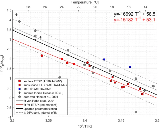
The dark production rates at the surface varied between 0.86 and 1.81 pmol L-1 h-1 along the northern part of the cruise track, and between 0.16 and 0.81 pmol L-1 h-1 in the four depth profiles below 50 m. The Arrhenius-type temperature dependency showed significantly increasing dark production rates with increasing temperature (Pearson’s test, p=5.66 x10⁻¹⁰). Dark production PD both at the surface and at depth along the cruise track (Fig. 4) is described by the following Arrhenius- 25
equation:
PD= a350∙exp�−15182T + 53.1� (7)
The Arrhenius-fit could not be improved using FDOM, DOSSPE or O2 instead of a350 (not shown). At station 5, the dark production rates at 50 and 136 m were larger than predicted for the temperature and the a350 present (Fig. 4).
11
The parameterization for dark production previously including only dark production rates from the North Atlantic, Mediterranean and North Sea (Von Hobe et al., 2001) was updated with the data from the ETSP and the Indian Ocean, and yields the following semi-empirical equation (eq. 8) (Fig. 4):
PD= a350∙exp�−16692T + 58.5� (8)
3.2.3 Diapycnal fluxes 5
The diapycnal fluxes of OCS within the water column were derived from measured concentration and diffusivity profiles.
OCS that was produced at the surface was mixed downwards in all four profiles. Diapycnal fluxes out of the mixed layer were always two or three orders of magnitude smaller than emissions to the atmosphere at stations 2, 5 and 7 with diapycnal fluxes of 8.2 x 10⁻⁴, 2.4 x 10⁻⁴ and 3.8 x 10⁻³ pmol s-1 m-2. An exception is station 18, where diapycnal fluxes (0.48 pmol s-1 m-2) were almost half of the air-sea flux (-1.0 pmol s-1 m-2).
10
3.2.4 Photoproduction
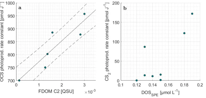
The photoproduction rate constants according to equation (6) were previously derived from a surface box model and have already been discussed in Lennartz et al. (2017). For days with concurrent measurements of FDOM (7, 8, 9, 10, 13, 16 October 2015), the correlation between photoproduction rate constant and humic-like FDOM C2 was significant (Pearson’s test, p=0.014, R²=0.81, Fig. 5a). The relationship was quantified by the following empirical equation (9):
15
p = 85.8 ∙[FDOM C2] + 828.76 (9)
with the photoproduction rate constant p [pmol J-1] and the concentration of the FDOM component C2 [QSU]. The correlation with a350 only explained a variance of R²=0.01.
20
OCS concentrations in the water column were simulated with the new module in the model environment of GOTM/FABM.
While the AQY of Weiss et al. (1995) yielded surface concentrations of a factor 3-6 too small compared to observations, the L17 simulation overestimated concentrations in all cases up to twofold (Fig. 3). Deviations between simulation and measurements were reduced by using the updated dark production rate of this study and the linear correlation between FDOM C2 and p shown in Fig. 5a (eq. 9, see section 3.2.2). At station 18, surface concentrations were simulated lower than 25
observed. The shapes of the concentration profiles were well reflected in the simulations except at station 5, where the subsurface concentration peaks at 55 m and 136 m were not adequately reproduced. Despite the different magnitude of the wavelength-resolved (W95) and wavelength-integrated (L17, L19) approaches, the shape of the photoproduction profile in the water column did not show major differences.
12
3.3 Carbon Disulfide (CS2)
3.3.1 Horizontal and vertical distribution
The surface concentration of CS2 during ASTRA-OMZ was in the lower picomolar range with an average of 17.8 ±8.9 pmol L-1 and displayed diurnal cycles only on some (e.g. 7 Oct 2015), but not at the majority of days (Fig. 3). The spatial pattern of sea surface concentrations was opposite to that of OCS, with highest concentrations distant from the shelf and lowest 5
closer to the shore. Highest surface concentrations of CS2 coincided with warm temperatures (Fig. 2b and 2c).
The concentration profiles of CS2 did not show a steep decrease with depth like OCS, but were more homogeneous (S-Fig. 3) apart from subsurface peaks below the mixed layer that occurred for example at stations 2, 5 and 18. The concentration in CS2 profiles down to about 200m was distinctly higher in profiles where upwelling did not occur (stations 1 to 13, ~20 pmol L-1) compared to stations in the Southern part of the cruise track (stations 15 to 18, ~10 pmol L-1). This difference in 10
concentrations throughout the water column reflected the pattern observed at the surface, where high concentrations coincide with high temperatures.
3.3.2 Diapycnal fluxes
The diapycnal fluxes of CS2 within the water column revealed highest production at the surface except for station 18. Within the water column, CS2 was redistributed downwards. Small in-situ sinks (stations 2, 7, and 18) and in-situ sources at 15
different water depths (stations 2 and 18) within the water column were required to maintain convergences/divergences under a steady state assumption. Fluxes out of the ML were 7.6 x 10⁻⁴, 3.3 x 10⁻⁴, 1.9 x10⁻³ and 0.98 pmol s-1 m-2 at stations 2, 5, 7 and 18 and thus 1-3 orders of magnitude smaller than fluxes to the atmosphere. At station 18, diapycnal fluxes out of the ML and emissions to the atmosphere were at a similar magnitude (0.98 and -1.0 pmol s-1 m-2 respectively).
3.3.3 Photoproduction of CS2 20
Photoproduction rate constants for CS2 were determined using an inverse set up of the surface box model analogous to OCS, but including only photoproduction and air-sea exchange as source and sink terms. The resulting photoproduction rate constants were between 5 to 70 times smaller than those of OCS. Opposite to OCS, the rate constants did not covary significantly with any FDOM component (p>>0.05). A weak trend was detected for DOSSPE (p=0.08, Spearman’s r²=0.44, n=8, Fig. 5), all other tested parameters did not show any correlation (FDOM C1-C4, CDOM).
25
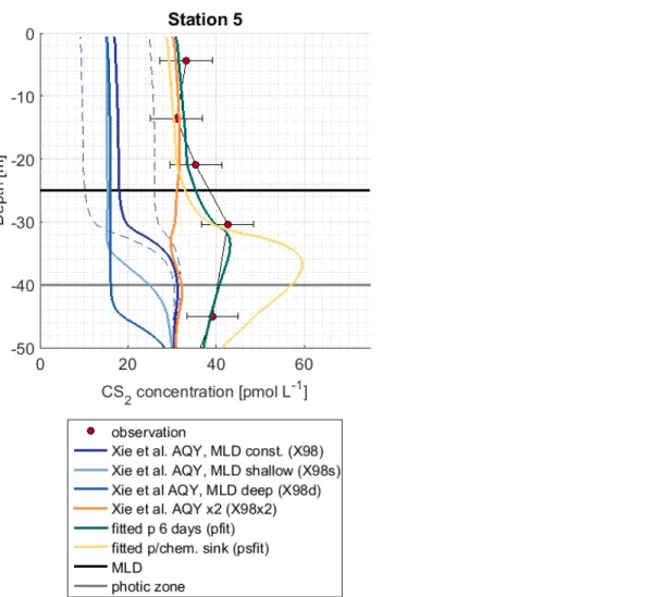
The shape of the CS2 concentration profiles was modelled for four stations (S-Fig. 2, supplements) with the scenarios described in Table 1. Concentrations in the mixed layer of stations 2,5 and 7 using the wavelength resolved AQY from Xie et al. (1998) yielded concentrations 4-6 times lower than observed (simulation X98).
The influence of mixed layer depth variations was tested in simulations X98d and X98s. Surface concentrations differed from the reference simulation X98 by <2.5 pmol L-1 (Fig. 6). The shape of the concentration profile, however, was sensitive 30
13
to mixed layer variations, as indicated by the sensitivity simulations X98d and X98s. In these artificially created test scenarios, concentrations accumulated below the bottom of the deepest mixed layer during the simulation period.
The subsurface concentration peak was investigated with 1) simulation X98x2 with the wavelength-dependent AQY by Xie et al. (1998) scaled by a factor of 2 so that it matches CS2 concentrations in the mixed layer, and 2) simulation pfit and psfit where a photoproduction rate constant in an integrated wavelength-approach (eq. 6) was fitted to observed profiles 5
(corresponding to an evenly distributed AQY across wavelengths from 300-400 nm). Simulation X98x2 does not reproduce the subsurface peak, whereas simulations ‘pfit’ and ‘psfit’ are two possible scenarios to reproduce the observed peak (Fig.
6).
4 Discussion
4.1 Carbonyl Sulfide 10
The four profiles at stations 2, 5, 7 and 18 represent the first observations of OCS profiles in the ETSP. They do not indicate any connection to a significant redox-sensitive process, as most profiles show a continuous decreasing shape as expected for photochemically produced compounds with a short lifetime in seawater. Station 5 was the only profile, which differed in shape. This profile was measured in an eddy where downward mixing occurred (Stramma et al., 2016), which may explain the increased concentrations at 55 m.
15
Dark production rates of up to 1.81 pmol L-1 h-1 in our study were at the upper end of the range of previously reported rates in the open ocean (Von Hobe et al., 2001; Ulshöfer et al., 1995; Ulshöfer et al., 1996; Flöck and Andreae, 1996; Von Hobe et al., 1999), but similar to those from the Mauritanian upwelling region (Von Hobe et al., 1999). Our results together with these previous studies show that tropical upwelling areas are globally important regions for OCS dark production, likely due to the combination of high a350 and moderate temperatures (15-18°C). The temperature dependency of the dark production 20
(eq. 7 and 8) is very similar to the one found by Von Hobe et al. (2001) in the North Atlantic, North Sea and Mediterranean (Fig. 4). The similarity points towards a ubiquitous process across different biogeochemical regimes, as the dependence of the production rate on temperature and a350 is very similar for an oligotrophic region like the Sargasso Sea (Von Hobe et al., 2001) or the Indian Ocean during the OASIS cruise (Lennartz et al., 2017) and a nutrient rich and biologically very productive region such as the ETSP. A strong similarity across different biogeochemical regimes favors the hypothesis of a 25
radical production pathway, which would be indifferent to the prevailing biological community. The radical pathway hypothesis is also supported by the fact that the fit in the Arrhenius-dependency could not be improved by other parameters than a350, and showed no influence to dissolved O2. The characteristics that make a molecule part of the CDOM pool, i.e.
unsaturated bonds and non-bonding orbitals, also favor radical formation. The results are in line with findings by Pos et al.
(1998) showing that these molecules can form radicals in the absence of light e.g. mediated by metal complexes. However, 30
the profile at station 5 provides some evidence that an additional process occurs in the subsurface. The concentration peak was visible in the up- and the downcast, but since we only observed it only once, we cannot conclusively rule out that the
14
OCS peak at 136 m is an artefact. Still, similar subsurface peaks have been reported from stations in the North Atlantic by Cutter et al. (2004). They concluded that dark production is connected to remineralization.
Diapycnal fluxes at stations 2, 5, 7 and 18 indicate downward mixing from the surface to greater depths in all profiles.
However, fluxes were several orders of magnitude smaller than emissions to the atmosphere, except for station 18. There, internal waves led to high diffusivities, which increased the flux at that station. Diapycnal fluxes will change diurnally with 5
the shape of the concentration profile and mixed layer variations, hence, the measurements here only represent a snapshot.
Still, the difference in magnitudes between air-sea exchange and diapycnal fluxes seems to be valid at varying times of the days and regions in the ETSP. Hence, neglecting diapycnal fluxes when calculating OCS concentrations in mixed layer box models leads only to minor overestimations of the concentrations.
An interesting finding is the significant correlation of the photoproduction rate constant p with FDOM C2 (humic-like 10
FDOM), but not with DOSSPE. OCS photoproduction is apparently not limited by an organic sulfur source but rather by humic substances potentially acting as photosensitizers or providing organic radicals as precursors. The humic-like FDOM component C2 is an abundant fluorophore in both marine (Catalá et al., 2015; Jørgensen et al., 2011), coastal (Cawley et al., 2012) and freshwater (Osburn et al., 2011) environments. This FDOM component seems to be especially abundant in the deep ocean (Catalá et al., 2015), which might be the reason for higher C2 surface concentrations in regions of upwelling, as 15
evident in our study and reported by Jørgensen et al. (2011). The significant correlation with humic-like fluorophores highlights the importance of upwelling and coastal regions for OCS photoproduction. The correlation to a350 on a regional scale explains much less of the variance compared to humic-like FDOM. On global scales, humic-like substances and CDOM a350 covary more strongly than on regional scales. Hence, the parameterization for p based on a350 can be improved using FDOM on the regional level.
20
Remarkable is also the absence of dissolved organic sulfur as a limiting factor, given a reported correlation of OCS and DOS in the Sargasso Sea where much higher DOS concentrations of ca. 0.4 µmol S L-1 were present (Cutter et al., 2004). It should be noted that the method to extract DOSSPE in our study does not recover all DOS compounds, and we cannot exclude the possibility that this influences the missing correlation between p and DOS. However, a possible explanation for the independence of OCS production from organic sulfur is a surplus of sulfur from other sources, such as sulfide. Based on 25
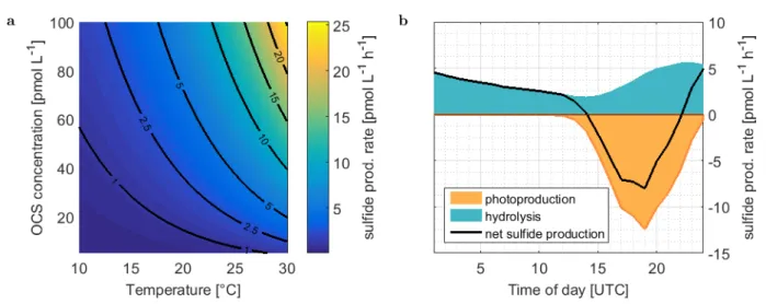
laboratory experiments, Pos et al. (1998) showed that the sulfur could be either derived from an organic or from an inorganic source, i.e. sulfide. Since hydrolysis of OCS itself produces sulfide, inorganic sulfur is available depending on the temperature-dependent hydrolysis rate. A missing correlation of p and DOSSPE is consistent with the reaction mechanism proposed by Pos et al. (1998), explicable by an existing sulfur-cycle between photoproduction and hydrolysis. Hydrolysis of OCS is one of the major producers of sulfide in the ocean (Shooter, 1999) and leads to higher sulfide production in warm 30
waters compared to colder regions (Fig. 7a). In warm tropical regions, hydrolysis might produce enough sulfide to sustain OCS photoproduction, resulting in a limitation by optically active DOM fractions such as the FDOM C2.
The production of sulfide by OCS hydrolysis and the sulfur demand by OCS photoproduction are illustrated in Fig. 7b based on our model output for an average day during the cruise ASTRA-OMZ. The integrated daily sulfur demand of
15
photoproduction (i.e. 75.8 pmol L-1) could theoretically be covered completely by inorganic sulfur generated from OCS hydrolysis (i.e. 85.8 pmol L-1). Due to different diel cycles of photoproduction and hydrolysis (Fig. 7b), the resulting net sulfide production is positive during nighttime and negative during daytime when sulfide is consumed. We cannot quantify the partitioning of the contribution between organic and inorganic sulfur for the production of OCS based on our data, but at least any sulfur that is lost to the atmosphere by emissions of OCS would need to be replenished from other sources, such as 5
DOS.
In addition, we used parameterizations from previously reported 0D box models and from this study to assess their applicability to biogeochemical models coupled to a 1D physical host model. It should be noted, however, that the surface data shown here have been used, along with other data, to derive the parameterization for the photoproduction rate constant in Lennartz et al. (2017). Photoproduction rates based on the wavelength-resolved simulation W95 underestimated observed 10
concentrations in all cases. A scaling factor for the AQY would be needed to explain observations. Such a scaling factor is implemented in the wavelength-integrated parameterization in Lennartz et al. (2017, simulation L17), yielding simulated concentrations closer to, but higher than observations (Fig. 3). The simulation using the updated dark production rate and scaling p with FDOM C2 (this study, L19) led to simulated concentrations closest to observations. Remaining deviations between simulated and observed profiles occur e.g. at station 5, possibly due to the reasons discussed above for dark 15
production rates. At station 18, vertical water displacements of up to 50m during one day were observed, most likely due to internal waves. This displacement could violate assumptions inherent to the 1D approach, i.e. influence of horizontal water transport. In general, our results show that simulating OCS concentrations in the water column is possible by applying surface box model parameterizations as local source and sink terms to a physical host model in the ETSP with its specific DOM conditions. The approach is similar to the 1D model by von Hobe et al. (2003) for the Sargasso Sea, but the updated 20
parameterizations yield a higher agreement in shape and actual concentrations of model simulation and observation.
4.2 Carbon Disulfide
The CS2 concentrations measured in the ETSP were higher than those observed during an Atlantic transect (Kettle et al., 2001, average 10.9 pmol L-1, n=744), and in the North Atlantic (13.4 pmol L-1) and the Pacific (14.6 pmol L-1) (Xie and Moore, 1999), but lower than those reported in a more recent transect through the Atlantic (Lennartz et al., 2017). High 25
concentrations of CS2 coincided with elevated temperatures at the surface in our and in previous studies. Xie et al. (1999) found a positive correlation between CS2 concentration and SST for the Pacific and the North Atlantic with a linear relationship of [CS2] = 0.39t +7.2 (t=temperature in °C). Daily averages of our data close to the shelf (n=8, from 12 Oct onwards) fall within this relationship. However, daily averaged concentrations were higher than predicted according to this relationship further away from the coast at the beginning of our cruise (n=4). Overall, we confirm that CS2 concentrations 30
increase with increasing temperatures, but the exact relationship varies spatially. Reasons for this relationship could result from e.g. temperature-driven decay of precursor molecules, but remain speculative.
16
The surface box model to determine photoproduction rate constants of CS2 is set-up as a very simple case, including only the processes of photoproduction and air-sea exchange. The rate constant p was only fitted for the increase in concentration during daylight, when photoproduction is expected to be much larger than potential other unknown, continuously acting sources or sinks. The photoproduction rate constant of CS2 was highest when high DOSSPE was present, indicating that the sulfur source might be limiting for this process. Organic sulfur is required to form CS2 even if one S-atom originates from an 5
inorganic S source (like for OCS). A potential mechanism could include a precursor with an existing C-S double or single bond that reacts with either another organic sulfur radical or sulfide. This mechanism would rationalize the correlation with DOS being present for CS2 and not for OCS. Laboratory studies showed that the organic sulfur compounds cystine, cysteine and (to a lesser extent) methionine are precursors for CS2 photochemistry (Xie et al., 1998). Such organic sulfur-containing molecules are rare in the marine environment (Ksionzek et al., 2016), which can explain the overall lower photoproduction 10
rate constant of CS2 compared to OCS. We found higher DOSSPE concentrations in the ETSP compared to other regions, but similar to DOSSPE concentrations in the Mauretanian upwelling reported by Ksionzek et al. (2016). There, elevated CS2
concentrations were reported as well (Kettle et al., 2001). This spatial pattern suggests that upwelling regions might be hot spots for CS2 photoproduction. It should be considered, however, that the extraction method used cannot recover all DOS compounds in seawater, so that the correlation between CS2 and DOSSPE may be influenced by the DOM composition.
15
Our simulation X98 at stations 2, 5, 7 and 18 underestimates mixed layer CS2 concentrations, indicating that the AQY most likely has to be scaled to match local conditions. These results corroborate findings by Kettle (2000) and Kettle et al. (2001), who showed that the photoproduction of CS2 was underestimated in some regions by the AQY from Xie et al. (1998). The scaling factor was on the order of 1-10 in Kettle’s studies, which is in line with our results (factor 2-4). In future model approaches, this photoproduction rate constant would need to be parameterized, and our results suggest that such 20
parameterizations may rely on DOS or, on a global scale, DOC (since DOS covaries globally with DOC).
The wavelength-dependence of the photochemical production is assessed with a 1D modelling approach, where the simulations ‘X98x2’ and ‘pfit’/’psfit’ reproduce surface concentrations, but differ in their wavelength-dependence of the photoproduction. In the simulation ‘X98x2’, the wavelength-dependent AQY was scaled to match surface concentrations, but failed to reproduce the observed subsurface peak at station 5, because photoproduction at wavelengths ~400 nm, that 25
penetrate below the ML was too low. In this scenario, another production process is needed to reproduce the observed profile. Similar conclusions were drawn by Xie et al. (1998). They suggested biological production, as the peaks coincided with the peak of chlorophyll a. However, we did neither find any correlation with chlorophyll a nor with marker pigments representing various phytoplankton functional types (data source described in Booge et al. (2018)). A potential other dynamic process, e.g. downward mixing, that influences both gases cannot be ruled out, as concentrations for OCS were also 30
higher than predicted around 50 m.
In our simulation ‘pfit’, a wavelength-integrated approach was adopted (eq. 6). It represents a scenario where photoproduction occured below the mixed layer, since substantial production takes place at higher wavelengths penetrating deeper into the water column. The accumulation occured because the production is detached from the air-sea exchange sink.
17
In this simulation, a period of 6 days was needed to accumulate enough CS2 below the mixed layer to reproduce observed concentrations. This period highly depended on the actual production at wavelengths around 400 nm and can thus vary. With allowing for an additional sink process below the mixed layer (psfit) corresponding to an additional degree of freedom, observations can also be reproduced. Hence, it is possible to explain observed subsurface peaks by 1) photoproduction alone, if higher production is assumed at wavelength around 400 nm, the peak maximum depending on accumulation time and 5
potential additional sink processes, or 2) via an additional production process only occurring shortly below the ML barrier, such as the biological production suggested by (Xie et al., 1999), or 3) by downward mixing processes related to mixed layer dynamics (given the long CS2 lifetime, such processes could be either slow but continuous mixing processes or strong one- time events such as storms). The process leading to the observed profiles thus remains inconclusive. Our results highlight the importance of Lagrangian experiments following the same water mass for compounds with a lifetime on the order of days.
10
Information on the conditions prior to the profile measurements are needed to conclusively interpret the location and accumulation of subsurface peaks.
CS2 was still detectable below 200 m, in concentrations around 5-10 pmol L-1 in shelf regions and around 20 pmol L-1 in open ocean regions (except station 1). The rather homogeneous concentrations below 200 m depth suggest slow in-situ degradation rates. As a result, physical processes resulting from currents, eddies or shelf processes might gain a higher 15
importance for the distribution of CS2 in the subsurface compared to the shorter lived gas OCS. With sinks potentially acting on long timescales, CS2 could possibly be transported from sources located further away, e.g. from contact to the sediment in shelf regions or subduced from the surface. Incubation experiments using isotopically labelled CS2 would be helpful to constrain source and sink processes independently.
5 Summary and conclusion
20
We show concurrent measurements of the gases OCS and CS2 together with sulfur-containing and optically active fractions of the DOM pool in the ETSP. The results indicate how the quality and composition of DOM influences the production processes of both gases, with implications for predicting their concentrations on regional and, potentially, global scales.
A parameterization for dark production of OCS is updated. The photoproduction rate constant of OCS co-varies regionally with humic-like FDOM, most likely as a precursor in a radical reaction mechanism. More observations of OCS with humic- 25
like DOM could help to improve parameterizations of OCS photoproduction. A possible explanation for the lack of correlation between the photoproduction rate constant and DOSSPE might be that OCS hydrolysis generates enough sulfide to recycle back to OCS during photoproduction. This cycle might be especially active in the ETSP, where warm temperatures increase the hydrolysis rate and, thus, the generation of sulfide, and abundant humic-like molecules further enhance photoproduction. In contrast to OCS, the availability of organic sulfur might be a limiting factor for the photochemical 30
production of CS2.
18
These different limitations of photochemical production of both gases have implications for the expected spatial pattern of their marine surface concentrations. Both, OCS dark and photochemical production, correlate with optically active parts of the DOM pool, which are abundant at high latitudes, coastal and upwelling regions. Also, OCS is degraded by hydrolysis most efficiently in warm regions such as the tropics, resulting in longer lifetimes in high latitudes. Highest concentrations are thus expected in coastal regions of high latitudes, which is in line with observations. Increasing CS2 photoproduction with 5
increasing DOSSPE concentrations suggests highest surface concentrations in tropical and subtropical regions, where highest DOC and DOS concentrations are expected. This spatial pattern is in line with the limited measurements available (Kettle et al., 2001). Regarding the tropical missing source of atmospheric OCS, the spatial pattern of oceanic emissions would then favour oxidation of emitted CS2 to OCS as a potential candidate. Our measurements likely represent CS2 concentrations from the upper end of the range of tropical concentrations, since they were performed in a region with high DOS abundance. As 10
an upper limit, a sulfur flux calculated with average values from this cruise (T=20.2°C, S=35, u10=7.3 m s-1, CS2=17.8 pmol L-1) assumed for the whole tropical ocean (30°N-30°S, 1.95 x10¹⁴ m²) results in an annual emissions of 268 Gg S as OCS.
This flux, which represents an additional 140 Gg S to the global sulfur flux of CS2 reported by Lennartz et al. (2017) is still too low to sustain a missing source of additional 400-600 Gg S yr-1 (800-1000 Gg S-1 yr-1 total oceanic OCS emissions).
Overall, we show that processes to model OCS distributions are well known and quantified and that the lifetime is 15
sufficiently short to extend the parameterizations of the box model to a 1D water column model. OCS process understanding is better than for CS2, for which sufficient process understanding to conclusively model subsurface concentrations is still lacking. Our results emphasize the importance of vertical dynamics for longer lived compounds such as CS2 compared to the short lived OCS.
This study highlights the need for more in-situ measurements of OCS and CS2 below the mixed layer in various 20
biogeochemical regimes together with fractions of the DOM pool, to improve the suggested quantitative relationships across larger DOM variations. Subsurface processes, especially for CS2, remain elusive and require concerted experimental and field studies.
Author contributions
S.T.L. and C.A.M. designed the study. Measurements and interpretation for essential parameters was performed by D.B.
25
(CS2), T.F. (microstructure profiles), R.G.-A. (PARAFAC), K.B.K. and B.P.K. (DOSSPE), A.B. (radiation), R.R. (CDOM absorption). S.T.L. performed the simulations with support from H.B.. S.T.L., C.A.M. and M.v.H. synthesised the data.
S.T.L. wrote the manuscript with contributions from all coauthors.
19
Acknowledgements
We acknowledge the help of the co-chief scientist, Damian Grundle and the crew and captain of the RV Sonne during ASTRA-OMZ to perform our measurements. This work was supported by the German Federal Ministry of Education and Research through the project ROMIC-THREAT (BMBF- FK01LG1217A and 01LG1217B), ROMIC- SPITFIRE (BMBF- FKZ: 01LG1205C) and SOPRAN, the DFG grants GR4731/2-1 and MA6297/3-1, as well as a PhD grant within the DFG- 5
Research Centre/Cluster of Excellence “The Ocean in the Earth System”. Additional funding for C.A.M. and S.T.L. came from the Helmholtz Young Investigator Group of C.A. M., TRASE-EC (VH-NG-819), from the Helmholtz Association through the President’s Initiative and Networking Fund and the GEOMAR Helmholtz-Zentrum für Ozeanforschung Kiel.
This work was co-funded by a PhD Miniproposal granted to S.T.L. from the Integrated School of Ocean Sciences (ISOS) of the Cluster of Excellence "The Future Ocean" at Kiel University, Germany, as well as GEOMAR Seedfunding. We thank 10
NASA Goddard Space Flight Center, Ocean Ecology Laboratory, Ocean Biology Processing Group for providing access to satellite data of CDOM from Aqua MODIS. We thank C. Schlundt for her help in analyzing CS2 samples and I. Stimac for her help in analyzing DOSSPE samples.
References
Berry, J., Wolf, A., Campbell, J. E., Baker, I., Blake, N., Blake, D., Denning, A. S., Kawa, S. R., Montzka, S. A., Seibt, U., 15 Stimler, K., Yakir, D., and Zhu, Z.: A coupled model of the global cycles of carbonyl sulfide and co2: A possible new
window on the carbon cycle, Journal of Geophysical Research: Biogeosciences, 118, 842-852, 10.1002/jgrg.20068, 2013.
Booge, D., Schlundt, C., Bracher, A., Endres, S., Zäncker, B., and Marandino, C. A.: Marine isoprene production and consumption in the mixed layer of the surface ocean – a field study over two oceanic regions, Biogeosciences, 15, 649-667, 20 10.5194/bg-15-649-2018, 2018.
Bruggeman, J., and Bolding, K.: A general framework for aquatic biogeochemical models, Environmental Modelling &
Software, 61, 249-265, http://dx.doi.org/10.1016/j.envsoft.2014.04.002, 2014.
25 Brühl, C., Lelieveld, J., Crutzen, P. J., and Tost, H.: The role of carbonyl sulphide as a source of stratospheric sulphate aerosol and its impact on climate, Atmos. Chem. Phys., 12, 1239-1253, 10.5194/acp-12-1239-2012, 2012.
Campbell, J. E., Carmichael, G. R., Chai, T., Mena-Carrasco, M., Tang, Y., Blake, D. R., Blake, N. J., Vay, S. A., Collatz, G. J., Baker, I., Berry, J. A., Montzka, S. A., Sweeney, C., Schnoor, J. L., and Stanier, C. O.: Photosynthetic control of 30 atmospheric carbonyl sulfide during the growing season, Science, 322, 1085-1088, 10.1126/science.1164015, 2008.
Catalá, T. S., Reche, I., Fuentes-Lema, A., Romera-Castillo, C., Nieto-Cid, M., Ortega-Retuerta, E., Calvo, E., Álvarez, M., Marrasé, C., Stedmon, C. A., and Álvarez-Salgado, X. A.: Turnover time of fluorescent dissolved organic matter in the dark global ocean, Nature Communications, 6, 5986, 10.1038/ncomms6986
35 https://www.nature.com/articles/ncomms6986#supplementary-information, 2015.
Cawley, K. M., Butler, K. D., Aiken, G. R., Larsen, L. G., Huntington, T. G., and McKnight, D. M.: Identifying fluorescent pulp mill effluent in the gulf of maine and its watershed, Marine Pollution Bulletin, 64, 1678-1687, 2012.
40
20