LECTURES ON TROPICAL CYCLONES

CYCLONES

Roger K. Smith

Date: June 2, 2006

Contents

1 OBSERVATIONS OF TROPICAL CYCLONES 5

1.1 Structure . . . . 5

1.1.1 Precipitation patterns, radar observations . . . . 9

1.1.2 Wind structure . . . . 11

1.1.3 Thermodynamic structure . . . . 11

1.1.4 Vertical cross-sections . . . . 12

1.1.5 Composite data . . . . 15

1.1.6 Strength, intensity and size . . . . 15

1.1.7 Asymmetries . . . . 17

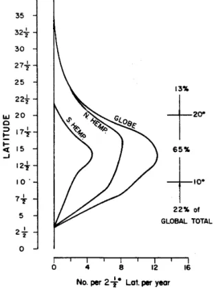
1.2 Formation regions . . . . 19

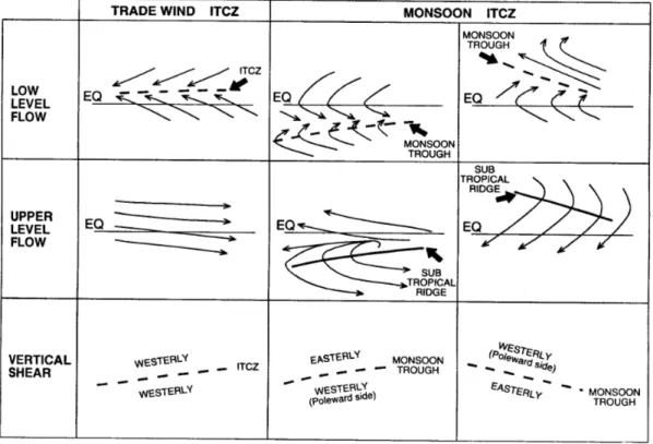
1.2.1 Large-scale conditions for formation . . . . 26

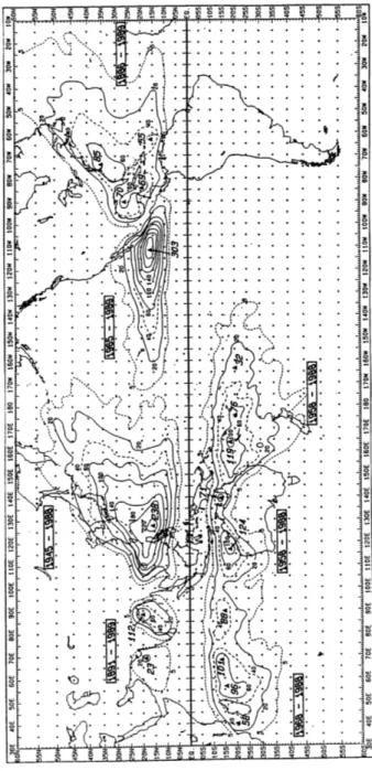
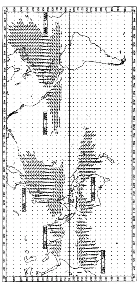
1.3 Tropical-cyclone tracks . . . . 27

2 DYNAMICS OF MATURE TROPICAL CYCLONES 30 2.1 The primary and secondary circulation . . . . 30

2.2 The equations of motion . . . . 30

2.3 The primary circulation . . . . 32

2.4 The tropical-cyclone boundary layer . . . . 34

2.5 Moist convection and the sloping eyewall . . . . 36

2.6 Buoyancy and generalized buoyancy . . . . 37

2.7 The tropical cyclone eye . . . . 40

2.8 Radiative cooling . . . . 41

2.9 Tropical cyclone intensity change . . . . 43

2.10 The secondary circulation . . . . 43

2.10.1 Ertel PV and the discriminant . . . . 47

2.10.2 The forcing term for ψ in terms of generalized buoyancy . . . 48

2.10.3 The Sawyer-Eliassen equation and toroidal vorticity equation . 48 2.10.4 Buoyancy relative to a balanced vortex . . . . 49

2.10.5 Buoyancy in axisymmetric balanced vortices . . . . 49

2.11 Origins of buoyancy in tropical cyclones . . . . 50

2.12 A balanced theory of vortex evolution . . . . 51

2.13 Appendix to Chapter 2 . . . . 51

2.13.1 The toroidal vorticity equation . . . . 51

2

3 A SIMPLE BOUNDARY LAYER MODEL 53

3.1 The boundary layer equations . . . . 53

3.2 Shallow convection . . . . 56

3.3 Starting conditions at large radius . . . . 56

3.4 Thermodynamic aspects . . . . 59

4 THE EMANUEL STEADY STATE HURRICANE MODEL 62 4.1 Region II . . . . 65

4.2 Region III . . . . 67

4.3 Region I and the complete solution . . . . 67

4.4 The tropical cyclone as a Carnot heat engine . . . . 69

4.5 The potential intensity of tropical cyclones . . . . 72

4.6 Appendix to Chapter 4 . . . . 78

4.6.1 Evaluation of the integral in Eq. (4.49) . . . . 78

5 TROPICAL CYCLONE MOTION 80 5.1 Vorticity-streamfunction method . . . . 80

5.2 The partitioning problem . . . . 81

5.3 Prototype problems . . . . 82

5.3.1 Symmetric vortex in a uniform flow . . . . 82

5.3.2 Vortex motion on a beta-plane . . . . 85

5.3.3 The effects of horizontal shear and deformation . . . . 94

5.4 The motion of baroclinic vortices . . . . 99

5.4.1 Vorticity tendency for a baroclinic vortex v (r, z ) in a zonal shear flow U (z). . . . 99

5.4.2 The effects of vertical shear . . . 106

5.5 Appendices to Chapter 5 . . . 107

5.5.1 Derivation of Eq. 5.16 . . . 107

5.5.2 Solution of Eq. 5.25 . . . 109

6 VORTEX ASYMMETRIES, VORTEX WAVES 111 6.1 Axisymmetrization . . . 111

6.2 Vortex Rossby waves . . . 116

6.3 Free waves on a resting basic state . . . 124

6.4 Free waves on barotropic vortices . . . 129

6.4.1 Disturbance equations . . . 129

6.5 The basic state: A PV inversion problem . . . 130

6.5.1 Wave-mean flow interaction . . . 131

7 MOIST PROCESSES 132 7.1 Idealized modelling studies . . . 132

7.2 Other modelling studies . . . 132

8 TROPICAL CYCLONE PREDICTION 133

9 ADVANCED TOPICS 134

9.1 Vortex stiffness . . . 134

9.2 Potential Radius coordinates . . . 134

9.3 Asymmetric balance theory . . . 134

10 Appendices 135 10.1 Thermodynamics . . . 135

10.1.1 Basic quantities . . . 135

10.1.2 CAPE and CIN . . . 136

10.1.3 Maxwell’s Equations . . . 137

10.2 Transformation of Euler’s equation to an accelerating frame of reference139 10.3 Angular momentum and vorticity fluxes . . . 141

10.4 References . . . 144

Chapter 1

OBSERVATIONS OF TROPICAL CYCLONES

Tropical cyclones are intense, cyclonically

-rotating, low-pressure weather systems that form over the tropical oceans. Intense means that near surface sustained

wind speeds exceed 17 ms

(60 km h

, 32 kn). Severe tropical cyclones with near surface sustained wind speeds equal to or exceeding 33 ms

(120 km h

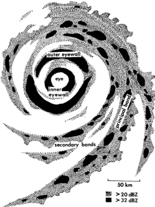
, 64 kn) are called hurricanes over the Atlantic Ocean, the East Pacific Ocean and the Caribbean Sea, and Typhoons over the Western North Pacific Ocean. Typically the strongest winds occur in a ring some tens of kilometres from the centre and there is a calm region near the centre, the eye, where winds are light, but for moving storms, the wind distribution may be asymmetric with the maximum winds in the forward right quadrant. The eye is so-called because it is normally free of cloud, except perhaps near the surface, but in a mature storm it is surrounded by a ring of deep convective cloud that slopes outwards with height. This is the so-called eyewall cloud. At larger radii from the centre, storms usually show spiral bands of convective cloud. Figure 1.1 shows a satellite view of the eye and eyewall of a mature typhoon, while Fig.

1.2 shows photographs looking out at the eyewall cloud from the eye during aircraft reconnaissance flights.

1.1 Structure

The mature tropical cyclone consists of a horizontal quasi-symmetric circulation on which is superposed a thermally-direct

vertical (transverse) circulation. These are sometimes referred to as the primary and secondary circulations, respectively, terms which were coined by Ooyama (1982). The combination of these two component circulations results in a spiralling motion. Figure 1.3 shows a schematic cross-section

1

Cyclonic means counterclockwise (clockwise) in the northern (southern) hemisphere.

2

The convention for the definition of sustained wind speed is a 10 min average value, except in the United States, which adopts a 1 min average.

3

Thermally direct means that warm air rising, a process that releases potential energy.

5

Figure 1.1: Infra-red satellite imagery of a typhoon.

of prominent cloud features in a mature cyclone including the eyewall clouds that surround the largely cloud-free eye at the centre of the storm; the spiral bands of deep convective outside the eyewall; and the cirrus canopy in the upper troposphere.

Other aspects of the storm structure are highlighted in Fig. 1.4. Air spirals into the storm at low levels, with much of the inflow confined to a shallow boundary layer, typically 500 m to 1 km deep, and it spirals out of the storm in the upper troposphere, where the circulation outside a radius of a few hundred kilometres is anticyclonic.

The spiralling motions are often evident in cloud patterns seen in satellite imagery and in radar reflectivity displays. The primary circulation is strongest at low levels in the eyewall cloud region and decreases in intensity with both radius and height as shown by the isotachs of mean tangential wind speed on the right-hand-side of the axis in Fig. 1.4. Superimposed on these isotachs are the isotherms, which show the warm core structure of the storm, with the largest temperatures in the eye. Outside the eye, most of the temperature excess is confined to the upper troposphere.

On the left side of the axis in Fig. 1.4 are shown the isolines of equivalent

potential temperature, θ

, referred to also as the moist isentropes. Note that there

(a)

(b)

Figure 1.2: Aerial photographs of the eye wall looking out from the eyes of (a) Hurricane Allen (1983), and (b) Typhoon Vera (19xx)

is a strong gradient of θ

in the eyewall region and that the moist isentropes slope

radially outwards with height. This important feature, which we make use of in

discussing the dynamics of tropical cyclones in section 2.10, is exemplified also by

the θ

-structure observed in Hurricane Inez (1966), shown in Fig. 1.5. Since θ

is

approximately conserved in moist flow, even in the presence of condensation, the

pattern of the isentropes reflects the ascent of air parcels in the eyewall from the

boundary layer beneath to the upper-level outflow. The large inward radial gradient

of θ

is a consequence of the rapid increase in the moisture flux from the ocean on

account of the rapid increase of wind speed with decreasing radius as the eyewall is

approached.

Figure 1.3: Schematic cross-section of cloud features in a mature tropical cyclone.

Vertical scale greatly exaggerated. (From Gentry, 1973)

Figure 1.4: Radial cross-section through an idealized, axisymmetric hurricane. On left: radial and vertical mass fluxes are indicated by arrows, equivalent potential temperature (K) by dashed lines. On right: tangential wind speed in m s

1 is indicated by solid lines and temperature in

C by dashed lines. (From Wallace and Hobbs, 1977 and adapted from Palm´ en and Newton, 1969)

The ”classical” structure of a tropical cyclone core is exemplified by that of Hur-

ricane Gilbert at 2200 UTC on 13 September 1988. At this time Gilbert was an

Figure 1.5: Vertical cross-sections of equivalent potential temperature (K) in Hurri- cane Inez of 1964 (From Hawkins and Imbembo 1976)

intense hurricane with a maximum wind speed in excess of 80 m s

and it had the lowest sea-level pressure ever measured (888 mb) in the Western Hemisphere. The following description is adapted from that of Willoughby (1995). The storm was especially well documented by data gathered from research aircraft penetrations.

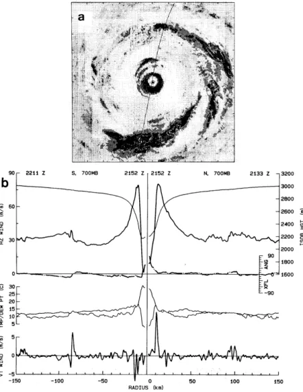
1.1.1 Precipitation patterns, radar observations

A composite of radar reflectivity observed in Gilbert’s core from one of the research aircraft is shown in Fig. 1.6. The eye is in the center of the picture, and is surrounded by the eyewall with maximum radar reflectivities of 40-47 dBZ

. The reflectivity in the eye is below the minimum detectable signal for the radar. During the flight, visual observation showed the eye to be free of clouds at and above flight level with blue sky visible overhead. Below flight level, broken stratocumulus in the lowest 1 km of the eye partially obscured the sea surface. In the radar image, the radius from the centre of the eye to the inner edge of the eyewall is about 8 km. The outer edge of the eyewall is less than 20 km from the center. Surrounding the eyewall is a ”moat” where the reflectivities are less than 25 dBZ, which is equivalent to a factor of more than 100 lower rainfall rates than in the eyewall. As the aircraft flew across the moat at 3 km altitude, it was in rain beneath an overcast sky, and low stratocumulus obscured the surface. Beyond the outer edge of the moat (75 km from

4

The decibel, abbreviated dBZ is a measure of the intensity of the backscattered radar beam

and is related to the intensity of precipitation in the storm.

Figure 1.6: (a) Plan-position indicator (PPI) radar reflectivity composite of Hurri- cane Gilbert at about 2200 UTC on 13 September 1988, when it was at maximum intensity near 19.9N, 83.5W. (b) Fight-level measurements from research aircraft.

The abscissa is distance along a north-south pass through the centre. The top panel shows wind speed (dark solid line), 700 mb height (light solid line), and crossing angle (tan

u/v, dash-dotted line). Winds are relative to the moving vortex centre.

The middle panel shows temperature (upper curve) and dewpoint. When T

> T , both are set to

(T + T

). The bottom panel shows vertical wind. (From Black and Willoughby 1992)

the centre), the radar image shows precipitation organized into spirals that appear

to be coalescing into a second ring of convection around the inner eye. Whereas

the maximum reflectivities in the spirals are about 45 dBZ, which is a value com-

parable with that in the eyewall, reflectivities are ≤ 30 dBZ over much of the area

outside the moat. Radar shows patterns of precipitation, but radar images contain important clues for visualization of the flow also. Echo-free areas, such as the eye and the moat, generally indicate vortex-scale descent. The highly reflective echoes contain both convective updrafts and precipitation-induced downdrafts. The indi- vidual echoes may be arranged in rings that encircle the centre, or in open spirals.

The lower reflectivities over most of the rings and spirals are stratiform rain falling from overhanging anvil cloud; the higher reflectivities are embedded convective cells.

Based upon a typical radar reflectivity-rainfall relationship

the rainfall rate is less than 4 mm h

in the stratiform areas and greater than 45 mm h

in the strong convective cells, which typically cover only a few percent of the hurricane as a whole.

Corresponding radial profiles of flight-level wind, 700 mb geopotential height, tem- perature, and dewpoint observed by the aircraft are shown in Fig. 1.6b. These are discussed below.

1.1.2 Wind structure

The strongest horizontal wind (> 80 m s

) is in the eyewall, only 12 km from the calm at the axis of rotation. This is typical of a tropical cyclone, although in weaker storms the radius maximum wind speed is larger, ranging up to 50 km or more.

Outside the eyewall, the wind drops abruptly to about 30 m s

at the outer edge of the moat and then rises to 35 m s

in the partial band of convection surrounding the moat. The cross-flow angle (tan

u/v, where u and v are the radial and tangential wind components) at 700 mb is < 10

. There is a tendency for radial flow toward the wind maxima from both the inside and the outside, which indicates that the horizontal wind converges into these features, even in the mid-troposphere. Not surprisingly, convective-scale vertical motions (updrafts), or on the south side of the eyewall in this case, downdrafts, often lie where the inflows and outflows converge just a kilometer or two radially outward from the horizontal wind maxima. The strongest vertical motions, even in this extremely intense hurricane, are only 5-10 m s

. There is a statistical tendency for the downdrafts to lie radially outward from the updrafts, as occurs, for example, 80 km south of Gilbert’s centre.

1.1.3 Thermodynamic structure

The air temperature shows a steady rise as the aircraft flies inwards towards the eyewall and then a rapid rise as it enters the eye. Thus the warmest temperatures are found in the eye itself, not in the eyewall clouds where the latent heat occurs.

These warm temperatures must arise, therefore, from subsidence in the eye. The dynamics of the eye and the reasons for this subsidence are discussed in section 2.7.

At most radii in Fig. 1.6b, the dewpoint depression

is on the order of 4

C.

5

Z = 300R

, where Z is the reflectivity (in mm

m

) and R is the rainfall rate (mm h

);

see Jorgensen and Willis 1982

6

The difference between the temperature and the dewpoint temperature

Figure 1.7: A dropsonde observation in the eye of Hurricane Hugo, near 14.7

N 54.8

W at 1838 UTC September 1989. Temperature is the right hand curve and dewpoint is the left. Nearly vertical curving lines are moist adiabats. Lines sloping up to the left are dry adiabats; those sloping up to the right are isotherms; and horizontal lines are isobars (From Willoughby 1995).

The air is saturated only where convective vertical motions pass through flight level.

Inside the eye, the temperature is greater than 28

C and the dewpoint is less than 0

C. These warm and dry conditions are typical of the eyes of extremely intense tropical cyclones. A sounding in the eye of Hurricane Hugo on 15 September 1989, when its structure was much like Gilbert’s even though its central pressure was 34 mb higher, is shown in Fig. 1.7. An inversion at 700 mb separates air with a dewpoint depression of about 20

C from saturated air that follows a moist adiabat down to the sea surface. Above the inversion, the air detrains from the eyewall near the tropopause and flows downward as part of a thermally indirect, forced subsidence in the eye. It is moistened a little by entrainment from the eyewall and evaporation of virga. Below the inversion, the air is cooler and nearly saturated as a result of inflow under the eyewall, inward mixing, and evaporation from the sea inside the eye.

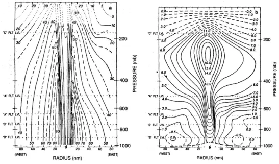
1.1.4 Vertical cross-sections

Research aircraft transects in Hurricane Hilda 1964 were obtained at five different

levels enabling the vertical structure of the storm to be documented. Cross-sections

of azimuthal wind and temperature anomaly are shown in Fig. 1.8. Again, as is

typical, the primary circulation in Hurricane Hilda (Fig. 1.8a) is strongest just

above the frictional boundary layer. Below 500 mb, it has little vertical shear, but in the upper troposphere, it becomes weaker and less symmetric, and the radial outflow is a large fraction of the swirling motion. Near the tropopause beyond 200 km radius, the vortex turns anticyclonic because of angular momentum loss to the sea on the inflow leg of the secondary circulation (Riehl 1963).

Figure 1.8: Vertical cross-sections of (a) azimuthal wind (kt), and (b) temperature anomaly (K) in Hurricane Hilda of 1964 (From Hawkins and Rubsam 1968)

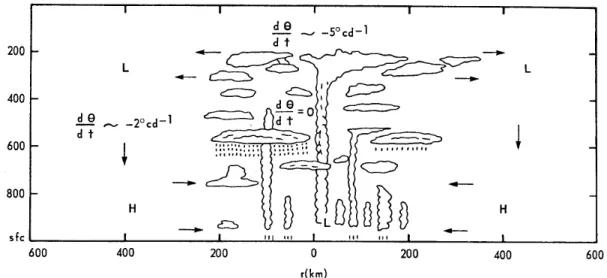
Figure 1.9 illustrates a schematic secondary circulation in a tropical cyclone such as Gilbert. This circulation is forced by an intense frictional destruction of angular momentum at the surface (section 2.8), by strong latent heat release in the inner eyewall clouds (section 2.5), weaker heating in the outer eyewall clouds, and extensive but weak cooling caused by frozen precipitation melting along the radar bright band

, and similarly extensive and weak heating due to condensation and freezing in the anvil above the bright band.

The low-level inflow in the heating-induced thermally direct gyres in Fig. 1.9 is distinct from the frictional inflow - see Fig. 1.10 below. The swirling wind in the friction layer is generally a little weaker than that just above. Thus, only the heating- induced inflow can supply an excess of angular momentum beyond that required to balance frictional loss. Observations show that the eyewall updrafts slope outward along constant angular momentum surfaces (Jorgensen 1984a,b; Marks and Houze 1987). The updraft slope from the vertical is the ratio of the vertical shear to the vertical component of the vorticity (Palm´en 1956) and has typical values of 30

-60

7

The bright band is a layer seen in vertical radar scans through cloud and coincides with the

melting layer just below the 0

C isotherm. Melting ice particles have enhanced reflectivity.

Figure 1.9: Schematic of the secondary circulation and precipitation distribution for a tropical cyclone similar to Hurricane Gilbert at the time in Fig. 1.6. (From Willoughby 1988)

(Black 1993), contrary to some claims that eyewalls are vertical (e.g. Shea and Gray 1973).

Outside the eye, latent heat release above the 0

C isotherm drives mesoscale updrafts. Below the 0

C isotherm, condensate loading and cooling due to melting of frozen hydrometeors drive mesoscale downdrafts. The mesoscale vertical velocities are typically tens of centimeters per second.

The secondary circulation controls the distribution of hydrometeors and radar reflectivity. Ascent is concentrated in convective updraft cores, which typically cover 10% of the area in the vortex core and more than half of the eyewall. The vertical velocity in the strongest 10% of the updraft cores averages 3-5 m s

. Except for

”supercell storms”

sometimes observed in tropical storms (Gentry et al. 1970; Black 1983), convective cells with updrafts > 20 m s

appear to be rare. Much of the condensate falls out of the outwardly sloping updrafts, so that the rain shafts are outside and below the region of ascent. The eyewall accounts for 25%-50% of the rainfall in the vortex core, but perhaps only 10% of the rainfall in the vortex as a whole. In the rain shafts, precipitation loading and, to a lesser extent, evaporation force convective downdrafts of a few meters per second. Any condensate that remains in the updrafts is distributed horizontally in the upper troposphere by the outflow.

It forms the central dense overcast that usually covers the tropical cyclone’s core, and much of it ultimately falls as snow to the melting level where it forms the radar brightband. Nearly all the updrafts glaciate by -5

C because of ice multiplication and entrainment of frozen hydrometeors (Black and Hallett 1986).

8

A supercell storm is one which has a single intense rotating updraft.

Above the boundary layer, the secondary circulation and distributions of radar reflectivity and hydrometeors are much like those in a tropical squall line (Houze and Betts 1981). They have the same extensive anvil, mesoscale up- and downdrafts, and brightband. The boundary layer flows and energy sources are, however, much different. As a squall line propagates, it draws its energy from the water vapour stored in the undisturbed boundary layer ahead of it, and leaves behind a cool wake that is capped by warm, dry mesoscale downdraft air under the anvil. However, as an eyewall propagates inward, but draws energy primarily from behind (outward) rather than ahead (inward). Frictional inflow feeds the updraft with latent heat extracted from the sea under the anvil. The reason for the difference between an eyewall and a squall line is the increased rate of air-sea interaction in the strong primary circulation of a tropical cyclone.

1.1.5 Composite data

Because of the difficulty and expense of gathering enough data for individual storms to construct vertical cross-sections such as those in Figs. 1.5 and 1.8, composite data sets have been constructed on the basis of data collected for very many similar storms at many time periods. The technique was pioneered by W. Gray and collaborators at the Colorado State University and is explained by Frank (1977). The idea is to construct eight octants of 45

azimuthal extent and eight radial bands extending from 0-1

, 1-3

, 3-5

, 5-7

, 9-11

, 11-13

and 13-15

. Data from individual soundings are assigned to one of these subregions according to their distance and geographical bearing relative to the storm centre. The data in these subregions are then averaged to define a composite storm.

Vertical cross-sections of the mean radial and tangential wind components in hurricanes, based on composite data from many storms are shown in Figs. 1.10.

Note that the radial wind component increases inwards with decreasing radius at low levels, is inward but relatively small through the bulk of the troposphere and is outward in the upper troposphere.

1.1.6 Strength, intensity and size

It is important to distinguish between the ”intensity” of the cyclone core and the

”strength” of the outer circulation. Intensity is conventionally measured in terms of maximum wind or minimum sea-level pressure; strength is a spatially-averaged wind speed over an annulus between 100 and 250 km from the cyclone centre. Another useful parameter is size, which may be defined as the average radius of gale force winds (≥17 m s

), or of the outer closed isobar (ROCI). Observations show that size and strength are strongly correlated, but neither is strongly correlated with intensity.

The climatology of size is well established for the Atlantic and North Pacific.

On average, typhoons are 1.5

lat. larger than Atlantic hurricanes. Small tropical

cyclones (ROCI < 2

lat.) are most frequent early in the season (August), and large

Figure 1.10: (From Gray, 1979; Frank 1977)

ones (ROCI > 10

lat.) late in the season (October). Large tropical cyclones are most common at 30

N, which is the average latitude of recurvature.

The life cycle of an Atlantic tropical cyclone begins with a formative stage during which the outer circulation contracts a little as the core intensifies. During the immature stage, the intensity increases to a maximum as the size remains constant.

In the mature stage, the tropical cyclone grows, but no longer intensifies. In the decaying stage, the inner core winds decrease as the circulation continues to grow.

The ROCI is typically 2.5

lat. in the immature stage and twice that value in the decaying stage a week e maximum intensity, start of rapid growth, and recurvature

of the track tend to coincide.

A detailed study of reconnaissance aircraft data from the western North Pacific confirms the low correlation between strength and intensity, and essentially no cor- relation between time changes in strength and intensity. That is, strength is equally likely to increase or decrease as a typhoon intensifies. Commonly, intensification pre- cedes strengthening, and weakening of the core precedes that of the outer circulation.

Classification of the observations by eye size [small (radius ≤ 15 km), medium (16-30 km), large (30-120 km), and eyewall absent] reveals correlations between intensity and strength, even though none could be found for the sample as a whole. These correlations may become evident because eye size acts as a proxy for phase of the typhoon life cycles.

Some relevant references are: Brand 1972; Merrill 1984; and Weatherford and Gray 1988a,b)

9

See section 1.XX

Figure 1.11: Streamline isotach analyses at 250, 500, and 850 mb for a composite Southern Hemisphere tropical cyclone, together with a typical visible satellite image.

(From Holland 1984)

1.1.7 Asymmetries

Normally only the inner-core regions of intense tropical cyclones show a significant degree of axial-symmetry. As shown in Fig. 1.11 for a Southern Hemisphere cyclone, the axisymmetric core is typically surrounded by a less symmetric outer vortex that merges into the synoptic environment. In the lower troposphere, the cyclonic circula- tion may extend more than 1000 km from the centre. The boundary between cyclonic and anticyclonic circulation slopes inward with height, so that the circulation in the upper troposphere is primarily anticyclonic except near the centre. The flow asym- metries in this region have a significant effect on the vortex motion (Chapter 5). In tropical cyclones that originate in the monsoon trough, the asymmetric flow is often associated with a band of convection that joins the cyclone to the trough (Holland 1984).

Spiral-shaped patterns of precipitation characterize radar and satellite images of

tropical cyclones (Fig. 1.12). The earliest radar observations of tropical cyclones

detected these bands, which are typically 5-50 km wide and 100-300 km long. Nev- ertheless, many aspects of their formation, dynamics, and interaction with the sym- metric vortex are still unresolved. The precipitation-free lanes between bands tend to be somewhat wider than the bands. As the tropical cyclone becomes more intense, the inward ends of the bands approach the center less steeply and then approximate arcs of circles.

Figure 1.12: Typical banded radar reflectivity pattern in a Northern Hemisphere tropical cyclone with 50-60 m s

maximum wind in a sheared environmental flow (From Willoughby 1988)

A dynamical distinction exists between convective bands that spiral outward from the center and convective rings that encircle the center. Because the bands often join a ring or appear to wrap around the centre (Dvorak 1984), this distinction is often difficult to make in radar or satellite images.

Although precipitation in some bands is largely from stratiform clouds, conden- sation in most bands tends to be concentrated in convective cells rather than spread over wide mesoscale areas. Convective elements form near the inner, upwind edges of the bands, move through the bands, and dissipate on the outward, downwind edges.

As the cells cross the band, they also move inward along the band. The dissipating elements feed an extensive anvil and generate widespread stratiform precipitation through horizontal advection of convective debris.

Some key observational studies of spiral bands are summarized by Willoughby

(1995), who gives a comprehensive list of references.

Dual-Doppler radar observations of a rainband in Supertyphoon Abby 1983 con- firmed inflow from the inward (concave) side, a locus of mesoscale ascent along the concave edge of the band, and a locus of mesoscale descent along the outer (convex) side. This pattern of inflow stemmed from the band’s steep inward crossing angle of 25

. The roots of the updrafts lay in convergence between the swirling flow and gust fronts that are produced by the downdrafts. The updrafts leaned outward from the typhoon center toward the convex side of the band and fed an extensive anvil that spread downwind from the band. The band moved more slowly than the surrounding winds, i.e., it propagated upwind. Even though the band was over land at 36

N, the equivalent potential temperature at the surface was 355 K, and this band should be considered representative of squall-line bands in hurricanes.

These Abby observations contrast with aircraft and radar observations of a ”band”

in Hurricane Floyd 1981. In the Floyd case, the low-level air spiraled inward more steeply than the band, so that the band intercepted the radial inflow on its outer, con- vex side. The inflow passed under the anvil between the convective-scale, precipitation- driven downdrafts to feed an updraft on the inner, concave side of the band. As in Typhoon Abby, the updraft sloped outward over the downdraft and fed an anvil extending away from the tropical cyclone center. The 20◦K decrease in low-level θ

across the band indicates that the band was a barrier to inflow. Independent obser- vations in Hurricane Earl emphasized that cooling and shallowing of the boundary layer occurred as the vortex-scale inflow passed under or between the cells of the bands (Fig. 1.13). This reduction in boundary-layer energy may have inhibited con- vection nearer the centre. Sometimes the band may draw air from both sides. An important difference between a convective ring and a spiral band is that the swirling wind feeds the updraft in a band from the concave side, whereas the radial flow feeds the updraft in a convective ring primarily from the convex side.

Some bands appear to move outward, while others maintain a fixed location relative to the translating tropical cyclone centre. Moving bands, and other convec- tive features, are frequently associated with cycloidal motion of the tropical cyclone centre, and intense asymmetric outbursts of convection (supercells) are observed to displace the tropical cyclone centre by tens of kilometres.

1.2 Formation regions

Tropical cyclones form in many parts of the world from initial convective distur-

bances sometimes referred to as cloud clusters. As the clusters evolve from a loosely

organized state into mature, intense storms, they pass through several characteristic

stages, but a uniform terminology does not exist to describe these stages over the

different regions of the globe. Indeed there has been much debate in the literature

about the meaning of such terms as ”tropical cyclogenesis”, ”tropical-cyclone for-

mation,” and ”tropical-cyclone development” (see e.g. McBride 1995). There are

differing opinions also as to when genesis has occurred and intensification has com-

Figure 1.13: Thermodynamic structure of a rainband in Hurricane Earl 1986. The grey outline shows the cloud boundary, and the contours show radar reflectivity.

Heavy horizontal and vertical arrows indicate the cross-band (V

) and convective vertical flows; lighter arrows indicate mesoscale subsidence. (From Powell 1990b)

Figure 1.14: Radar echo pattern seen in Hurricane Alicia (1983) labelled according

to the schematic to Fig. 1.14. Contours are for 25 and 40 dBZ. (From Marks and

Houze 1987)

menced. McBride op. cit. remarks that the existence of a (warm) core region can be identified by the time that the system is classified as a tropical cyclone (i.e., mean wind speeds exceeding 17.5 m s

or 34 kt). Further development of the maximum wind speeds beyond 17.5 m s

will be referred to as intensification. This stage includes the evolution of the core into a well-defined radar eye.

Generally a larger scale (i.e., thousand kilometre) vortex already exists when the core develops and much of the research into tropical cyclone formation has examined the formation of the large-scale vortex in which the core forms. The distinction be- tween core formation and large-scale vortex formation is important because different dynamical processes may be involved.

Here we follow McBride and refer to tropical cyclone formation as the transition from the cloud cluster state to the tropical cyclone stage with winds exceeding 17.5 m s

. Changes in wind speed of the outer vortex are referred to as outer structure change, or strength change, or size change.

Figure 1.15: Locations of tropical cyclone formation over a 20-year period. (From Gray, 1975)

Each year approximately 80 tropical cyclones occur throughout the world, and about two thirds of these reach the severe tropical cyclone stage. Gray (1975) doc- umented the initial detection points of each cyclone for a 20-year period fig. 1.15.

Preferred regions of formation are over the tropical oceans and it is significant that these coincide broadly with regions of high sea surface temperatures (SSTs) (1.16).

The warmest waters occur in the Western Pacific, the so-called ”warm pool region”,

while the ocean temperatures in the Southeast Pacific is relatively cold. Indeed, cli-

matological studies by Palm´en (1948, 1957) and Gray (1995) have shown that tropical

cyclogenesis occurs only in regions where the sea surface temperature is above 26.5

C

and where the depth of the 26

C isotherm is 60 m or more. No formations occur

within about 2.5

lat. of the equator. Most of the formations (87%) occur between

20

N and 20

S (Fig. 1.17). Another interesting statistic is the frequency of tropical

cyclones per 100 years within any point as shown in Fig. 1.18.

Figure 1.16: Annual mean sea-surface temperature (

C). (From ???)

About two thirds of all cyclones occur in the Northern Hemisphere, and twice as many tropical cyclones occur in the Eastern as in the Western Hemisphere. These differences are due in part to the absence of tropical cyclones in the South Atlantic and the eastern South Pacific. Tropical cyclones are seasonal phenomena, and most basins have a maximum frequency of formation during the late summer to early fall period. The Southern Hemisphere peak occurs in January to March and the Northern Hemisphere peak is from July to September. The most active region is the Northwest Pacific Ocean, where typhoons occur in all seasons.

The seasonal distribution of formation locations is governed by two major factors.

One is the association between tropical cyclone formation and SST, with the highest values of SST occurring during the late summer. Notice that regions of warm water also extend farther from the equator in the Northern Hemisphere in association with the Gulf Stream and the Kuroshio currents. However, SST is only one factor, as is evidenced by the absence of cyclones in the South Atlantic despite similar values of SST at certain times of the year.

The second factor in the seasonal distributions is related to the seasonal vari- ations in the location of the monsoon trough. As discussed by Gray (1968), the Inter-Tropical Convergence Zone (ITCZ), which extends semi-continuously around the globe, may occur as a convergence line between trade easterlies from the North- ern and Southern Hemispheres, or as a convergence zone in westerly monsoon flow.

In this latter configuration, the monsoon westerlies usually have trade easterlies on

Figure 1.17: Latitudes at which initial disturbances that later became tropical cy- clones were first detected. (From Gray 1975)

their poleward side. The shear line separating the monsoon westerlies from easter- lies is known as the monsoon trough or monsoon shear line and is a climatologically preferred region for tropical cyclone formation. Typical upper- and lower-level flow patterns for the two modes of the ITCZ are illustrated schematically in Fig. 1.19.

The trade convergence line of the ITCZ typically has large vertical wind shear. When monsoon westerlies are present, the low-level monsoon shear line is overlain (in the mean seasonal pattern) by the upper-level subtropical ridge. In western North Pa- cific, the ridge above the monsoon trough during the summer is called the subequato- rial ridge. This configuration of trade easterlies overlain with westerlies and monsoon westerlies overlain with easterlies gives a (seasonal-mean) vertical wind shear close to zero, with westerly shear on the poleward side and easterly shear on the equatorward side (bottom panel. Fig. 1.19).

The only region of cyclone formation not associated with a monsoon trough is the North Atlantic. Possible explanations for this anomaly are discussed below.

In the first global climatology of tropical cyclogenesis, Gray (1968, 1975, 1979) found that cyclone formation is related to six environmental factors:

(i) large values of low-level relative vorticity;

Figure 1.18: Frequency of tropical cyclones per 100 years within 140 km of any point.

Solid triangles indicate maxima, with values shown. Period of record used is shown in boxes for each basin. (From WMO, 1993)

(ii) a location at least a few degrees poleward of the equator, giving a significant value of planetary vorticity;

(iii) weak vertical shear of the horizontal winds; iv) sea-surface temperatures (SSTs)

exceeding 26

C, and a deep thermocline;

Figure 1.19: Schematics of trade-wind (left) and monsoon-type (two right columns) ITCZ flow regimes. The monsoon regimes are subdivided into those typical of the Australian/Southeast Indian Ocean ITCZ during January (middle) and the western North Pacific basin during August (right). Vertical wind shear between the low-level and upper-level flow is indicated in the lower panels.

(v) conditional instability through a deep atmospheric layer; and

(vi) large values of relative humidity in the lower and middle troposphere.

The first three factors are functions of the horizontal dynamics, while the last

three are thermodynamic parameters. Gray defined the product of (i), (ii), and (iii)

to be the dynamic potential for cyclone development, while the product of (iv), (v),

and (vi) may be considered the thermodynamic potential. The diagnosed tropical

cyclone formation frequency derived by Gray (1975) using the above parameters

is quite similar to the observed formation locations in (Fig. 1.15). However, the

combination or the above six parameters were ”tuned” to agree with the mean sea-

sonal and geographical distributions of tropical cyclone development. As discussed

by Gray (1975) and McBride (1981a), the thermodynamic parameters vary slowly

in time and would be expected to remain above any threshold values necessary for

tropical cyclone development throughout the cyclone season. On the other hand,

the dynamic potential can change dramatically through synoptic activity. Thus, it

was hypothesized by Gray that cyclones form only during periods when the dynamic potential attains a magnitude above its regional climatological mean.

Frank (1987) noted that the above six environmental parameters are not inde- pendent. In the tropics, regions of high sea-surface temperatures are invariably cor- related with conditional instability due to the weak horizontal temperature gradients in the lower troposphere. High humidities in the middle levels also tend to occur in convective clusters over warm waters, and virtually all areas with widespread deep convection are associated with mean ascending motion. Thus, Frank reduced the list to four parameters by combining (i) and (ii) into the absolute vorticity at low levels, deleting (v), and adding mean upward vertical motion to (vi). A number of obser- vational studies have derived parameters relevant to the potential of an individual disturbance to develop into a cyclone.

1.2.1 Large-scale conditions for formation

The observational studies have isolated a number of synoptic-scale aspects that have an important role in the formation process:

(i) Tropical cyclones form from pre-existing disturbances containing abundant deep convection;

(ii) The pre-existing disturbance must acquire a warm core thermal structure through- out the troposphere;

(iii) Formation is preceded by an increase of lower tropospheric relative vorticity over a horizontal scale of approximately 1000 to 2000 km;

(iv) A necessary condition for cyclone formation is a large-scale environment with small vertical wind shear;

(v) An early indicator that cyclone formation has begun is the appearance of curved banding features of the deep convection in the incipient disturbance;

(vi) The inner core of the cyclone may originate as a mid-level meso-vortex that has formed in association with a pre-existing mesoscale area of altostratus (i.e., a Mesoscale Convective System or MCS); and

(vii) Formation often occurs in conjunction with an interaction between the incipient disturbance and an upper-tropospheric trough.

Evidence for these seven observations are discussed in detail by McBride (1995).

1.3 Tropical-cyclone tracks

Figure 1.20 shows the tracks of all tropical cyclones (maximum winds > 17 m s

)

for the period 1979-1988 and Fig. 1.21 shows the mean direction of all hurricanes

during the period indicated. Tropical cyclones form over the warm tropical oceans

and typically move westwards and polewards, although tracks of individual storms

can be quite erratic. To a first approximation tropical cyclones are steered by a mass-

weighted average of the broadscale winds through the depth of the troposphere. It

is common for storms that reach sufficiently high latitudes to recurve and move

eastwards. Tropical cyclones rapidly lose their intensity when they move over land,

but they often continue to produce copious amounts of rain. In many cases of

landfalling storms, the majority of damage is caused by widespread flooding rather

than by strong winds. Near the coast, however, much damage may be caused by

high winds and by coastal storm surges. The dynamics of tropical-cyclone motion is

discussed in Chapter 5.

Figure 1.20: Tracks of all tropical cyclones (maximum winds > 17 ms

) for the

period 1979-1988. (From WMO, 1993)

Figure 1.21: Mean direction of tropical cyclone motion over the periods indicated.

(From WMO, 1993)

Chapter 2

DYNAMICS OF MATURE TROPICAL CYCLONES

2.1 The primary and secondary circulation

To a good first approximation the mature tropical cyclone consists of a horizon- tal quasi-symmetric circulation on which is superposed a thermally-direct vertical (transverse) circulation. These are sometimes referred to as the ”primary circula- tion” and ”secondary circulation”, respectively, terms which were coined by Ooyama (1982). The former refers to the tangential flow rotating about the central axis, and the latter to the ”in-up-and-out circulation” (low and middle level inflow, upper- level outflow). When these two components are combined, the picture emerges of air parcels spiralling inwards, upwards and outwards. The combined spiralling cir- culation is energetically direct because the rising branch of the secondary circulation near the centre is warmer than the subsiding branch, which occurs at large radial distances (radii > 500 km).

In this chapter we examine the dynamics of the spiralling circulation of tropical cyclones on the basis of the physical laws governing fluid motion and thermody- namic processes that occur. For simplicity we study the dynamics of a stationary axisymmetric hurricane-like vortex. In later chapters we consider the dynamics of tropical-cyclone motion and examine the asymmetric features of storms. We start by giving an overall picture of the dynamics and then go into detail about particular important aspects. First we introduce the governing equations and the important concept of buoyancy.

2.2 The equations of motion

To begin with we consider the full hydrostatic equations of motion, but with the density tendency in the continuity equation omitted. The primitive equations of motion comprising the horizontal momentum equation, the hydrostatic equation,

30

the continuity equation, the thermodynamic equation and the equation of states for frictionless motion in a rotating frame of reference on an f -plane may be expressed in cylindrical polar coordinates, (r, λ, z), as:

∂u

∂t + u ∂u

∂r + v r

∂u

∂λ + w ∂u

∂z − v

r − f v = − 1 ρ

∂p

∂r , (2.1)

∂v

∂t + u ∂v

∂r + v r

∂v

∂λ + w ∂v

∂z + uv

r + f u = − 1 ρr

∂p

∂λ , (2.2)

∂w

∂t + u ∂w

∂r + v r

∂w

∂λ + w ∂w

∂z = − 1 ρ

∂p

∂z − g, (2.3)

1 r

∂ρru

∂r + 1 r

∂ρv

∂λ + ∂ρw

∂z = 0, (2.4)

∂θ

∂t + u ∂θ

∂r + v r

∂θ

∂λ + w ∂θ

∂z = ˙ θ (2.5)

ρ = p

π

/(R

θ) (2.6)

where (u, v, w) is the velocity vector in component form, ρ is the air density, f is the Coriolis parameter, p is the pressure, θ is the potential temperature ˙ θ is the diabatic heating rate, π = (p/p

)

is the Exner function, R

is the specific gas constant for dry air, κ = R

/c

, c

is the specific heat at constant pressure, and p

= 1000 mb.

The temperature is defined by T = πθ. For tropical-cyclone scale motions it is a good approximation to make the hydrostatic approximation, whereupon Eq. (2.3) reduces to

∂p

∂z = −ρg. (2.7)

Multiplication of Eq. (2.2) by r and a little manipulation leads to the equation

∂M

∂t + u ∂M

∂r + v r

∂M

∂λ + w ∂M

∂z = − r ρ

∂p

∂λ , (2.8)

where

M = rv + 1

2 f r

, (2.9)

is the absolute angular momentum per unit mass of an air parcel about the rotation axis. If the flow is axisymmetric (and frictionless), the right-hand-side of (2.8) is zero and the absolute angular momentum is conserved.

Exercise 2.1 Assuming the most general form of the mass conservation equation:

∂ρ

∂t + 1 r

∂ (ρru)

∂r + 1 r

∂(ρv)

∂λ + ∂(ρw)

∂z = 0,

show that the absolute angular momentum per unit volume, M

= ρ

µ rv + 1

2 f r

¶ , satisfies the equation:

∂M

∂t + 1 r

∂(ruM

)

∂r + 1 r

∂ (vM

)

∂λ + ∂(wM

)

∂z = −r ∂p

∂λ .

2.3 The primary circulation

Important aspects of the basic structure of a mature tropical cyclone can be deduced from two simple equations that express an exact balance of forces in the vertical and radial directions. These equations enable one to develop a simple theory for the primary circulation.

Figure 2.1: Schematic diagram illustrating the gradient wind force balance in the primary circulation of a tropical cyclone.

Let us assume that the flow is steady (∂/∂t ≡ 0) and let us ignore the secondary circulation, i.e. we assume that the radial velocity is identically zero (see Fig. 2.1).

Then Eq. (2.1) reduces to the gradient wind equation:

v

r + f v = 1 ρ

∂p

∂r . (2.10)

The force balance expressed by this equation is called gradient wind balance.

Willoughby (1990) has shown that, in the free atmosphere, the azimuthal-mean tan-

gential circulation of tropical cyclones is in gradient balance to a good approximation.

Taking (∂/∂z)[ρ× Eq. (2.10)] and (∂/∂r)[Eq. (2.7)] and eliminating the pressure we obtain the thermal wind equation

g ∂ ln ρ

∂r + C ∂ ln ρ

∂z = − ∂C

∂z . (2.11)

where we have defined

C = v

r + f v (2.12)

to represent the sum of the centrifugal and Coriolis forces per unit mass. Equation (2.11) is a linear first-order partial differential equation for ln ρ. The characteristics of the equation satisfy

dz dr = C

g . (2.13)

The characteristics are just the isobaric surfaces, because a small displacement (dr, dz) along an isobaric surface satisfies (∂p/∂r)dr + (∂p/∂z)dz = 0. Then, us- ing the equations for hydrostatic balance (∂p/∂z = −gρ) and gradient wind balance (∂p/∂r = Cρ) gives the equation for the characteristics. Alternatively, note that the pressure gradient per unit mass, (1/ρ)(∂p/∂r, 0, ∂p/∂z) equals (C, 0, −g), which defines the ”generalized gravity”, g

; see Fig. 2.4. The density variation along a characteristic is governed by the equation

d

dr ln ρ = − 1 g

∂C

∂z . (2.14)

Given the vertical density profile, ρ

(z), Eqs. (2.13) and (2.14) can be integrated inwards along the isobars to obtain the balanced axisymmetric density and pressure distributions. In particular, Eq. (2.13) gives the height of the pressure surface that has the value p

(z), say, at radius R.

Since ∂C/∂z = (2v/r + f )(∂v/∂z), it follows from (2.14) that for a barotropic vortex (∂v/∂z = 0), ρ is constant along an isobaric surface, i.e. ρ = ρ(p), whereupon T

is a constant also.

The thermal wind equation (2.11), or equivalently Eq. (2.14), shows that in a cyclonic vortex in the northern hemisphere (v > 0) with tangential wind speed that decays with height (∂v/∂z < 0), log ρ and hence ρ decrease with decreasing radius along the isobaric surface. Thus the virtual temperature T

(r, z) and θ increase and the vortex is warm cored (i.e. ∂T

/∂r < 0). This prediction of the thermal wind equation is consistent with the observation that tropical cyclones are warm- cored systems, and that the tangential wind speed decreases with altitude. If the tangential wind speed were to increase with height (∂v/∂z > 0) the vortex would be cold cored. Note that the characteristics dip down as the axis is approached on account of Eq. (2.13). The reason for the warm core structure of tropical cyclones is discussed in section 2.5.

The analysis above shows that any steady vortical flow with velocity field u =

(0, v(r, z), 0) is a solution of the basic equation set (2.1) - (2.6), when the density field

satisfies (2.11). Willoughby’s observational evidence that the primary circulation of a hurricane is approximately in gradient wind balance makes the foregoing analysis a good start in understanding the structure of this circulation. However the solution neglects the secondary circulation associated with nonzero u and w and it neglects the effects of friction near the sea surface. These are topics of subsequent subsections.

Exercise 2.2 Show that in terms of the Exner function, Eqs. (2.10) and (2.7) may be written as

χC = c

∂π

∂r and − χg = c

∂π

∂z , (2.15)

respectively.

Exercise 2.3 Show that Eq. (2.11) may be reformulated as

g ∂(ln χ)

∂r + C ∂(ln χ)

∂z = − ∂C

∂z . (2.16)

where χ = 1/θ.

It is instructive to compare the magnitude of the centrifugal and Coriolis terms in Eq. (2.1), their ratio being

Ro(r) = v

f r . (2.17)

This equation defines a local Rossby number for the flow. Let r

be radius of maxi- mum tangential wind speed of a tropical cyclone and v

the tangential wind speed at this radius. Then Ro is typically on the order of 40 ÷ (40 × 10

× 5 × 10

) = 20, typical values for r

and v

being 40 km and 40 m s

, respectively. It follows that the inner core region of a tropical cyclone is approximately in cyclostrophic balance, i.e. the Coriolis forces are small compared with the centrifugal forces. However, at a radius of 200 km, where the wind speeds may be on the order of 10 m s

, Ro ≈ 1 and these two forces are comparable. As the radius increases further, the circulation becomes more and more geostrophic, i.e. Ro becomes small compared with unity and the Coriolis forces become dominant.

2.4 The tropical-cyclone boundary layer

It turns out that the effects of surface friction in a tropical cyclone have a dramatic

influence not only on the flow in the layer in which friction acts, the so-called bound-

ary layer, but also on the flow above this layer. The boundary layer is typically about

500 m deep. One obvious effect of friction is to reduce the tangential wind speed near the surface, and therefore the centrifugal and Coriolis forces. However, a scale analysis shows that it has little effect on the pressure field so that the radial pressure gradient in the boundary layer is approximately the same as that immediately above the layer (see e.g. Smith 1968). Thus there is a net inward force on air parcels in the boundary layer, which drives inflow in the layer (Fig. 2.2). Far from the rotation axis, both the inflow velocity and the radial mass flux increase with decreasing radius and this leads to forced subsidence above the boundary layer. At inner radii, where the inflow and mass flux begin to decline, air is discharged from the boundary layer into the vortex above. In other words, the presence of the boundary layer forces ver- tical motion in the main part of the vortex above the boundary layer. In the tropical cyclone, the air in the boundary layer is moistened as it spirals inwards over the warm ocean. This moistening elevates the pseudo-equivalent potential temperature of the boundary-layer air, θ

, so that ∂θ

/∂r < 0. We consider now the fate of this moist air and return in Chapter 3 to examine in detail the dynamics and thermodynamics of the boundary layer. There we show that given the tangential wind speed distrib- ution for a steady axisymmetric vortex, one can determine the radial distribution of the vertically-averaged wind speed components in the boundary layer as functions of radius as well as the induced vertical velocity at the top of the boundary layer.

Given also the vertically-averaged temperature and specific humidity at some large radius and the sea surface temperature beneath the vortex, one can determine the radial variation of the vertically-averaged θ

in the boundary layer.

Figure 2.2: Schematic diagram illustrating the disruption of gradient wind balance

by friction in the boundary layer leaving a net inward pressure gradient that drives

the secondary circulation with inflow in the boundary layer and outflow above it.

2.5 Moist convection and the sloping eyewall

When the inward-spiralling moisture-laden air is forced upwards out of the boundary layer in the inner core region, it expands and cools. Condensation rapidly ensues and as the air continues to rise in the eyewall clouds, latent heat is released and a significant fraction of the condensed water falls out of the clouds as precipitation. The latent heat release is responsible for the warm core in the cyclone, but only a small fraction of the heat released is manifest as an elevated temperature perturbation at a particular height; most of it is offset by the adiabatic cooling that occurs as air parcels rise and expand. We may think of the effect of the heat release on the temperature field as follows. To a first approximation, ascending air parcels conserve their θ

as indicated in Fig. 2.3. Since the air in the eyewall clouds is saturated, the virtual temperature of an air parcel at a particular pressure level is a monotonically- increasing function of its θ

, which, in turn, is equal to the θ

it had when it left the boundary layer. Therefore, at least in the eyewall cloud region the radial gradient of T

(z) is determined by the radial gradient of θ

at the top of the boundary layer, which as noted above is negative. In other words, at any level in the cloudy region, (∂T

/∂r)

< 0, which explains why the tropical cyclone has a warm core, at least outside the eye. The reason that the eye is warm also is examined in section 2.7. The discussion section 2.4 indicates that the boundary layer in a mature hurricane controls not only the rate at which air ascends at a particular radius, but determines also the radial gradient of virtual temperature (and hence density) above the boundary layer, at least in regions of ascent.

From mass continuity, the air that converges in the boundary layer must flow outwards above the boundary layer, a fact that accounts for the outward slope of the eyewall and of air parcel trajectories. Ascending air parcels approximately conserve their absolute angular momentum, M , as well as their θ

so that (absolute) angular momentum surfaces and the moist isentropes are approximately coincident (at least where there is cloud) and these surfaces slope outwards with height as indicated schematically in Fig. 2.3.

We emphasize that in the foregoing picture of the warm-core structure of a trop- ical cyclone, the latent heat release in clouds serves merely to maintain the conser- vation of pseudo-moist entropy characterized by θ

along air-parcel trajectories. The warm-core itself is seen as a result of the increase in θ

with decreasing radius as determined by the thermodynamic processes in the boundary layer, which are exam- ined in detail in Chapter 3. This picture was first proposed by Emanuel (1986) and forms the basis for his steady model for the tropical cyclone described in Chapter 4.

Many early papers consider the role of latent heat release as providing local buoyancy in the eye-wall clouds and suggest that it is this buoyancy that ”drives”

the secondary circulation. We shall see that this explanation is raises many questions.

For example the temperature in the eyewall clouds is typically less than in the eye.

Moreover, we have seen that much of the temperature field of the tropical cyclone

resides in thermal wind balance. To examine these questions in more detail we need

Figure 2.3: Schematic diagram of the secondary circulation of a mature tropical cyclone showing the eye and the eyewall clouds. Air spirals inwards in a shallow boundary layer near the sea surface, picking up moisture as it does so. The absolute angular momentum, M , and equivalent potential temperature, θ

of an air parcel is conserved after the parcel leaves the boundary layer and ascends in the eyewall clouds.

The precise values of these quantities depend on the radius at which the parcel exits the boundary layer. At radii beyond the eyewall cloud, shallow convection plays an important role in moistening and cooling the lower troposphere above the boundary layer and warming and drying the boundary layer as indicated.

to review the concept of air-parcel buoyancy, especially in the context of rapidly- rotating vortices. This is the subject of the next section.

2.6 Buoyancy and generalized buoyancy

The buoyancy of an air parcel in a density-stratified air layer is defined as the differ- ence between the weight of air displaced by the parcel (the upward thrust according to Archimedes principle) and the weight of the parcel itself. This quantity is normally expressed per unit mass of the air parcel under consideration, i.e.

b = −g (ρ − ρ

)

ρ , (2.18)

where ρ is the density of the parcel, ρ

= ρ

(z) is the density of the environment at

the same height z as the parcel, and g is the acceleration due to gravity. Here and

elsewhere the vertical coordinate z is defined to increase in the direction opposite to

gravity. The calculation of the upward thrust assumes that the pressure within the

air parcel is the same as that of its environment at the same level, an assumption that is invalid a rapidly-rotating vortex. In the latter case one can define a gener- alized buoyancy force, which acts normal to the isobaric surface intersecting the air parcel and which is proportional to the density difference between the parcel and its environment along that surface (see below).

A similar expression for the buoyancy force given in (2.18) may be obtained by starting from the vertical momentum equation and replacing the pressure p by the sum of a reference pressure p

and a perturbation pressure, p

. The former is taken to be in hydrostatic balance with a prescribed reference density ρ

, which is often taken, for example, as the density profile in the environment. In real situations, the environmental density is not uniquely defined, but could be taken as the horizontally- averaged density over some large domain surrounding the air parcel. Neglecting frictional forces, the vertical acceleration per unit mass can be written alternatively

as Dw

Dt = − 1 ρ

∂p

∂z − g or, Dw Dt = − 1

ρ

∂p

∂z + b (2.19)

where w is the vertical velocity, D/Dt is the material derivative, and t is the time presents a similar derivation, but makes the anelastic approximation (Ogura and Phillips, 1962), in which the density in the denominator of (2.18) is approximated by that in the environment. Clearly, the sum of the vertical pressure gradient and gravitational force per unit mass acting on an air parcel is equal to the sum of the vertical gradient of perturbation pressure and the buoyancy force, where the latter is calculated from Eq. (2.18) by comparing densities at constant height. The expression for b in (2.19) has the same form as that in (2.18), but with ρ

in place of ρ

. However, the derivation circumvents the need to assume that the local (parcel) pressure equals the environmental pressure when calculating b, which, as noted above, is not valid for a rapidly-rotating vortex. The foregoing decomposition indicates that, in general, the buoyancy force is not uniquely defined because it depends on the (arbitrary) choice of a reference density. However, the sum of the buoyancy force and the perturbation pressure gradient per unit mass is unique. If the motion is hydrostatic, the perturbation pressure gradient and the buoyancy force are equal and opposite, but they remain non-unique.

Using the gas law (p = ρR

T and the usual definition of virtual potential tem- perature, the buoyancy force per unit mass can be written as

b = g

· (θ − θ

)

θ

− (κ − 1) p

p

¸

, (2.20)

where θ is the virtual potential temperature of the air parcel in K and θ

is the

corresponding reference value. The second term on the right-hand-side of (2.20)

is sometimes referred to as the “dynamic buoyancy”, but in some sense this is a

misnomer since buoyancy depends fundamentally on the density perturbation and

this term simply corrects the calculation of the density perturbation based on the

virtual potential temperature perturbation. If the perturbation pressure gradient