Chapter 2
DYNAMICS OF MATURE TROPICAL CYCLONES
2.1 The primary and secondary circulation
The mature tropical cyclone consists of a horizontal quasi-symmetric circulation on which is superposed a thermally-direct vertical (transverse) circulation. These are sometimes referred to as the primary and secondary circulations, respectively, terms which were coined by Ooyama (1982). The combined spiralling circulation is ener- getically direct because the rising branch of the secondary circulation near the centre is warmer than the subsiding branch, which occurs at large radial distances (radii
>500 km). In this chapter we examine the dynamics of the spiralling circulation of tropical cyclones on the basis of the physical laws governing fluid motion and thermo- dynamic processes that occur. In particular we study the dynamics of a stationary axisymmetric hurricane-like vortex. In later chapters we consider the dynamics of tropical-cyclone motion and examine the asymmetric features of storms. We begin by giving an overall picture of the dynamics and then go into detail about particular important aspects.
2.2 The equations of motion
To begin with we consider the full hydrostatic equations of motion, but with the density tendency in the continuity equation omitted. The primitive equations of motion comprising the horizontal momentum equation, the hydrostatic equation, the continuity equation, the thermodynamic equation and the equation of states for frictionless motion in a rotating frame of reference on an f-plane may be expressed in cylindrical polar coordinates, (r, λ, z), as:
∂u
∂t +u∂u
∂r + v r
∂u
∂λ +w∂u
∂z − v2
r −f v =−1 ρ
∂p
∂r, (2.1)
30
∂v
∂t +u∂v
∂r + v r
∂v
∂λ +w∂v
∂z + uv
r +f u=− 1 ρr
∂p
∂λ, (2.2)
∂w
∂t +u∂w
∂r + v r
∂w
∂λ +w∂w
∂z =−1 ρ
∂p
∂z −g, (2.3)
1 r
∂ρru
∂r +1 r
∂ρv
∂λ +∂ρw
∂z = 0, (2.4)
∂θ
∂t +u∂θ
∂r +v r
∂θ
∂λ +w∂θ
∂z = ˙θ (2.5)
ρ=p∗πκ1−1/(Rθ) (2.6) where (u, v, w) is the velocity vector in component form,ρ is the air density,f is the Coriolis parameter, pis the pressure, θ is the potential temperature ˙θ is the diabatic heating rate, π = (p/p∗)κ is the Exner function, R is the specific gas constant, κ = R/cp, cp is the specific heat at constant pressure, and p∗ = 1000 mb. The temperature is defined by T = πθ. For tropical-cyclone scale motions it is a good approximation to make the hydrostatic approximation, whereupon Eq. (2.3) reduces
to ∂p
∂z =−ρg. (2.7)
Multiplication of Eq. (2.2) by r and a little manipulation leads to the equation
∂M
∂t +u∂M
∂r + v r
∂M
∂λ +w∂M
∂z =−1 ρ
∂p
∂λ, (2.8)
where
M =rv+1
2r2f, (2.9)
is the absolute angular momentum per unit mass of an air parcel about the rotation axis. If the flow is axisymmetric (and frictionless), the right-hand-side of (2.8) is zero and the absolute angular momentum is conserved.
Exercise 2.1 Assuming the most general form of the mass conservation equation:
∂ρ
∂t +1 r
∂(ρru)
∂r + 1 r
∂(ρv)
∂λ + ∂(ρw)
∂z = 0, show that the absolute angular momentum per unit volume,
Mv =ρ µ
rv+ 1 2r2f
¶ ,
satisfies the equation:
∂Mv
∂t +1 r
∂(ruMv)
∂r +1 r
∂(vMv)
∂λ +∂(wMv)
∂z =−∂p
∂λ.
2.3 Buoyancy
The buoyancy of an air parcel in a density-stratified air layer is defined as the differ- ence between the weight of air displaced by the parcel (the upward thrust according to Archimedes principle) and the weight of the parcel itself. This quantity is normally expressed per unit mass of the air parcel under consideration, i.e.
b=−g(ρ−ρa)
ρ , (2.10)
where ρ is the density of the parcel, ρa=ρa(z) is the density of the environment at the same height z as the parcel, and g is the acceleration due to gravity. Here and elsewhere the vertical coordinate z is defined to increase in the direction opposite to gravity. The calculation of the upward thrust assumes that the pressure within the air parcel is the same as that of its environment at the same level, an assumption that may be unjustified in a rapidly-rotating vortex. In the latter case one can define a generalized buoyancy force, which acts normal to the isobaric surface intersecting the air parcel and which is proportional to the density difference between the parcel and its environment along that surface (see below).
A similar expression for the buoyancy force given in (2.10) may be obtained by starting from the vertical momentum equation and replacing the pressure p by the sum of a reference pressure pref and a perturbation pressure, p0. The former is taken to be in hydrostatic balance with a prescribed reference density ρref, which is often taken, for example, as the density profile in the environment. In real situations, the environmental density is not uniquely defined, but could be taken as the horizontally- averaged density over some large domain surrounding the air parcel. Neglecting frictional forces, the vertical acceleration per unit mass can be written alternatively
as Dw
Dt =−1 ρ
∂p
∂z −g or, Dw Dt =−1
ρ
∂p0
∂z +b (2.11)
where w is the vertical velocity, D/Dt is the material derivative, and t is the time presents a similar derivation, but makes the anelastic approximation (Ogura and Phillips, 1962), in which the density in the denominator of (2.10) is approximated by that in the environment. Clearly, the sum of the vertical pressure gradient and gravitational force per unit mass acting on an air parcel is equal to the sum of the vertical gradient of perturbation pressure and the buoyancy force, where the latter is calculated from Eq. (2.10) by comparing densities at constant height. The expres- sion for b in (2.11) has the same form as that in (2.10), but with ρref in place of ρa. However, the derivation circumvents the need to assume that the local (parcel) pressure equals the environmental pressure when calculating b. The foregoing de- composition indicates that, in general, the buoyancy force is not uniquely defined because it depends on the (arbitrary) choice of a reference density. However, the sum of the buoyancy force and the perturbation pressure gradient per unit mass is unique. If the motion is hydrostatic, the perturbation pressure gradient and the buoyancy force are equal and opposite, but they remain non-unique.
Using the gas law (p=ρRT, where R is the specific gas constant) and the usual definition of virtual potential temperature, the buoyancy force per unit mass can be written as
b =g
·(θ−θref)
θref −(κ−1) p0 pref
¸
, (2.12)
where θ is the virtual potential temperature of the air parcel in K and θref is the corresponding reference value. The second term on the right-hand-side of (2.12) is sometimes referred to as the “dynamic buoyancy”, but in some sense this is a misnomer since buoyancy depends fundamentally on the density perturbation and this term simply corrects the calculation of the density perturbation based on the virtual potential temperature perturbation. If the perturbation pressure gradient terms in (2.11) are written in terms of the Exner function and/or its perturbation, the second term in (2.12) does not appear in the expression for buoyancy. The expression (2.12) is valid also in a rapidly rotating vortex, but as shown in section 2.5, there exists then a radial component of buoyancy as well. When clouds are involved it may be advantageous to include the drag of hydrometeors in the definition of buoyancy, but we omit this additional effect here.
2.4 The primary circulation
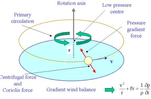
Figure 2.1: Schematic diagram illustrating the gradient wind force balance in the primary circulation of a tropical cyclone.
To begin with we assume that the flow is steady (∂/∂t ≡ 0) and we ignore the secondary circulation, i.e. we assume that the radial velocity is identically zero (see
Fig. 2.1). Then Eq. (2.1) reduces to the gradient wind equation:
v2
r +f v= 1 ρ
∂p
∂r. (2.13)
In the data for Hurricane Gilbert shown in Fig. 1.11b, the strongest radial gradi- ent of the 700 mb geopotential height roughly coincides with the maximum swirling wind, which suggests that the wind may be in gradient balance with the mass field.
In fact gradient balance prevailed in the mid-troposphere in Gilbert to within a root-mean-squared deviation of ±4m s−1 (Willoughby, 1995, p28).
Taking (∂/∂z)[ρ×Eq. (2.13)] and (∂/∂r)[Eq. (2.2)] and eliminating the pressure we obtain the thermal wind equation
g∂(lnρ)
∂r +C∂(lnρ)
∂z =−∂C
∂z. (2.14)
where we have defined
C = v2
r +f v (2.15)
to represent the sum of the centrifugal and Coriolis forces per unit mass. This is a linear first-order partial differential equation for lnρ. The characteristics of the equation satisfy
dz dr = C
g . (2.16)
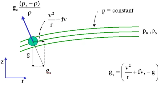
The characteristics are just the isobaric surfaces, because a small displacement (dr, dz) along an isobaric surface satisfies (∂p/∂r)dr+(∂p/∂z)dz = 0. Using the equa- tions for hydrostatic balance,∂p/∂z =−gρ, and gradient wind balance,∂p/∂r=Cρ, gives the equation for the characteristics. Alternatively, note that the pressure gradi- ent per unit mass, (1/ρ)(∂p/∂r,0, ∂p/∂z) = (C,0,−g), which defines the ”generalized gravity”, ge; see Fig. 2.2. The density variation along the characteristics is governed by the equation
d drln
µ ρ ρa
=−1 g
∂C
∂z. (2.17)
Given the vertical density profile, ρa(z), these Eqs. (2.16) and (2.17) can be inte- grated inwards along the isobars to obtain the balanced axisymmetric density and pressure distributions. Thus Eq. (2.16) gives the height of the pressure surface that has the value pa(z), say, at radius R.
It follows from (2.17) that for a barotropic vortex (∂v/∂z = 0), ρ is constant along an isobaric surface, i.e. ρ =ρ(p), whereupon Tv is a constant also. Note that
∂C/∂z = (2v/r+f)(∂v/∂z).
The thermal wind equation (2.14) or (2.17) shows also that for a cyclonic vortex (v >0) withdv/dz <0, log(ρ/ρa) and henceρdecrease with decreasing radius along the isobaric surface so that the virtual temperatureTv(r, z) andθ increase. Thus the vortex is warm cored. Conversely, if dv/dz > 0, the vortex is cold cored. Certainly
Figure 2.2: Schematic radial-height cross-section of isobaric surfaces in a rapidly- rotating vortex showing the forces on an air parcel including the gravitational force g, per unit mass, and the sum of the centrifugal and Coriolis forces C = v2/r+f v per unit mass. Note that the isobaric surfaces are normal to the local ”generalized gravitational force” ge = (C,0,−g). The Archimedes force −geρref slopes upwards and inwards while the weight geρ slopes downwards and outwards. Thus the net buoyancy force acting on the parcel per unit mass is|ge|(ρref−ρ)/ρin the direction shown.
Eq. (2.14) is consistent with the observation that tropical cyclones are warm-cored systems (i.e. ∂Tv/∂r <0), and that the tangential wind speed decreases with altitude (∂v/∂z <0). Note that on account of Eq. (2.16), the characteristics dip down as the axis is approached. The reason for the warm core structure is discussed in section 2.5.
The analysis above shows that any steady vortical flow with velocity field u = (0, v(r, z),0) is a solution of the basic equation set (2.1) - (2.6), when the density field satisfies (2.14). Willoughby (1990) has shown from observations that the primary circulation of a hurricane is approximately in gradient wind balance so the foregoing analysis is a good start in understanding the structure of this circulation. However the solution neglects the secondary circulation associated with nonzero uand w and it neglects the effects of friction near the sea surface. These are topics of subsequent subsections.
Exercise 2.2 Show that in terms of the Exner function, Eqs. (2.13) and (2.7) may be written as
χC =cp
∂π
∂r and −χg =cp
∂π
∂z, (2.18)
respectively.
Exercise 2.3Show that Eq. (2.14) may be reformulated as
g∂(lnχ)
∂r +C∂(lnχ)
∂z =−∂C
∂z. (2.19)
where χ= 1/θ.
It is instructive to compare the magnitude of the centrifugal and Coriolis terms in Eq. (2.1), their ratio being
Ro(r) = v
f r. (2.20)
This equation defines a local Rossby number for the flow. At the radius of maxi- mum tangential wind speed, rm, the tangential wind speed at this radius, vm, Ro is typically on the order of 40÷(40×103×5×10−5) = 20, typical values for rm and vm being 40 km and 40 m s−1, respectively. It follows that the inner core region of a tropical cyclone is approximately in cyclostrophic balance, i.e. the Coriolis forces are relatively small. However, at a radius of 200 km, where the wind speeds may be on the order of 10 m s−1, Ro≈ 1 and Coriolis forces are comparable with centrifu- gal forces. As the radius increases further, the circulation becomes more and more geostrophic, i.e. Ro becomes small compared with unity.
2.5 Generalized buoyancy
In a rapidly-rotating, axisymmetric vortex, an air parcel experiences not only the gravitational force, but also the radial forceC =v2/r+f v, where v is the tangential wind component at radius r. If the vortex is in hydrostatic and gradient wind balance, the isobaric surfaces slope in the vertical and are normal to the effective gravity, ge = (C,0,−g), expressed in cylindrical coordinates (r, λ, z) (see Fig. 2.2).
The Archimedes force acting on the parcel is then−geρref and the effective weight of the parcel is geρ, where ρref is now the far-field (reference-) density along the same isobaric surface as the parcel. Accordingly, we may define a generalized buoyancy force per unit mass:
b =geρ−ρref
ρ , (2.21)
analogous to the derivation of (2.10). Note that unless v(v+rf) < 0, fluid parcels that are lighter than their environment have an inward-directed component of gen- eralized buoyancy force as well as an upward component, while heavier parcels have an outward component as well as a downward component. This result provides the theoretical background for a centrifuge.
2.6 The tropical-cyclone boundary layer
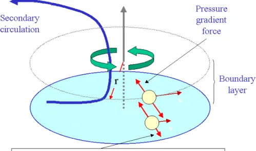
It turns out that the effects of surface friction in a tropical cyclone have a dramatic influence not only on the flow in the layer where friction acts, the so-called boundary layer, but also on the flow above this layer. The boundary layer is typically about 500 m deep. One obvious effect of friction is to reduce the tangential wind speed near the surface. However, a scale analysis shows that it has little effect on the pressure field so that the radial pressure gradient in the boundary layer is approximately the same as that immediately above the layer (see e.g. Smith 1968). However, the centrifugal and Coriolis forces are reduced by friction leaving a net inward force on air parcels within the boundary layer, which leads to inflow within the layer (Fig. 2.3). Far from the rotation axis, both the inflow velocity and the radial mass flux increase with decreasing radius and this leads to forced subsidence above the boundary layer. At inner radii, where the inflow and mass flux begin to decline, air is discharged from the boundary layer into the vortex above. In other words, the presence of the boundary layer forces vertical motion in the vortex above the boundary layer. In the tropical cyclone, the air in the boundary layer is moistened as it spirals inwards over the warm ocean. The moistening elevates the pseudo-equivalent potential temperature of the boundary-layer air, θeb, so that ∂θeb/∂r < 0. We consider now the fate of this moist air and return in section 2.9 to examine in detail the dynamics and thermodynamics of the boundary layer. There we show that given the tangential wind speed distribution for a steady axisymmetric vortex, one can determine the radial distribution of the vertically-averaged wind speed components in the boundary layer as functions of radius as well as the induced vertical velocity at the top of the boundary layer. Given also the vertically-averaged temperature and specific humidity at some large radius and the sea surface temperature beneath the vortex, one can determine the radial variation of the vertically-averaged θeb in the boundary layer.
2.7 Moist convection and the sloping eyewall
When the inward-spiralling moisture-laden air is forced upwards out of the bound- ary layer in the inner core region, it expands and cools and condensation rapidly occurs. As the air continues to rise in the eyewall clouds, latent heat is released and a significant fraction of the condensed water falls out of the clouds as precip- itation. The latent heat release is responsible for the warm core in the cyclone, but only a small fraction of the heat released appears as an elevated temperature perturbation at a particular height; most of it is balanced by the adiabatic cooling that occurs as air parcels continue to rise and expand. We may think of the effect on the temperature field as follows. To a first approximation, ascending air parcels conserve their θe as indicated in Fig. 2.4. Since the air in the eyewall clouds is saturated, the virtual temperature of an air parcel at a particular pressure level is a monotonically-increasing function of its θe, which, in turn, is equal to the θe it had when it left the boundary layer. Therefore, at least in the eyewall cloud region the
Figure 2.3: Schematic diagram illustrating the disruption of gradient wind balance by friction in the boundary layer leaving a net inward pressure gradient that drives the secondary circulation with inflow in the boundary layer and outflow above it.
radial gradient of Tv(p) is determined by the radial gradient of θe at the top of the boundary layer, which as noted above is negative. In other words, at any level in the cloudy region, (∂Tv/∂r)p <0, which explains why the tropical cyclone has a warm core outside the eye. The reason that the eye is warm also is discussed in the next section. The discussion in section 2.4 indicates that the boundary layer in a mature hurricane controls not only the rate at which air ascends at a particular radius, but determines also the radial gradient of virtual temperature (and hence density) above the boundary layer, at least in regions of ascent.
From mass continuity, the air that converges in the boundary layer must flow outwards above the boundary layer, a fact that accounts for the outward slope of the eyewall and of air parcel trajectories. Ascending air parcels approximately conserve their absolute angular momentum, M, as well as their θe so that (absolute) angular momentum surfaces and the moist isentropes are approximately coincident (at least where there is cloud) and these surfaces slope outwards with height as indicated schematically in Fig. 2.4.
2.8 The tropical cyclone eye
As we have seen, the eye is a cloud free region surrounding the storm axis where the air temperature is warmest. Therefore, it would be reasonable to surmise that the air within it has undergone descent during the formative stages of the cyclone, and that
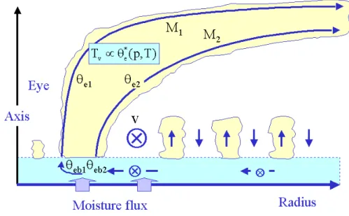
Figure 2.4: Schematic diagram of the secondary circulation of a mature tropical cyclone showing the eye and the eyewall clouds. Air spirals inwards in a shallow boundary layer near the sea surface, picking up moisture as it does so. The absolute angular momentum, M, and equivalent potential temperature, θe of an air parcel is conserved after the parcel leaves the boundary layer and ascends in the eyewall clouds.
The precise values of these quantities depend on the radius at which the parcel exits the boundary layer. At radii beyond the eyewall cloud, shallow convection plays an important role in moistening and cooling the lower troposphere above the boundary layer and warming and drying the boundary layer as indicated.
possibly it continues to descend. The question then is: why doesn’t the inflowing air spiral in as far as the axis of rotation. We address this question later, but first note that eye formation is consistent with other observed features of the tropical cyclone circulation. The following discussion is based on that of Smith (1980). Assuming that the primary circulation is in gradient wind balance, we may integrate Eq. (2.13) with radius to obtain a relationship between the pressure perturbation at a given height z on the axis to the tangential wind field distribution, i.e:
p(0, z) = p(∞, z)− Z ∞
0
ρ(v2
r +f v)dr, (2.22)
where p(∞, z) is the environmental pressure at the same height. Differentiating Eq.
(2.22) with respect to height and dividing by the density gives the perturbation pressure gradient per unit mass along the vortex axis:
−1 ρ
∂(p−p∞)
∂z =−1 ρ
∂
∂z Z ∞
0
ρ(v2
r +f v)dr. (2.23) Observations in tropical cyclones show that the tangential wind speed decreases
with height above the boundary layer and that the vortex widens with height in the sense that the radius of the maximum tangential wind speed increases with height (see Fig. 1.11). This behaviour, which is consistent with outward-slanting absolute angular momentum surfaces as discussed above, implies that the integral on the right-hand-side of Eq. (2.23) decreases with height. Then Eq. (2.23) shows that there must be a downward-directed perturbation pressure gradient force along the vortex axis. This perturbation pressure gradient tends to drive subsidence along and near to the axis to form the eye. However, as this air subsides, it is compressed and warms relative to air at the same level outside the eye and thereby becomes locally buoyant (i.e. relative to the air outside the eye). This upward buoyancy approximately balances the downward directed (perturbation) pressure gradient so that the actual subsidence results from a small residual force. In essence the flow remains close to hydrostatic balance.
As the vortex strengthens, the downward pressure gradient must increase and the residual force must be downwards to drive further subsidence. On the other hand, if the vortex weakens, the residual force must be upwards, allowing the air to re-ascend.
In the steady state, the residual force must be zero and there is no longer a need for up- or down motion in the eye, although, in reality there may be motion in the eye associated with turbulent mixing across the eyewall or with asymmetric instabilities within the eye.
It is not possible to measure the vertical velocity that occur in the eye, but one can make certain inferences about the origin of air parcels in the eye from their ther- modynamic characteristics, which can be measured (see e.g. Willoughby, 1995).Note that ∂T /∂p)s∗ is just the temperature lapse rate as a function of pressure along a moist adiabat.
2.9 A model for the boundary layer
We consider now a simple model for the tropical cyclone boundary layer as described by Smith (2003). The boundary layer equations for a steady axisymmetric vortex in a homogeneous fluid on an f-plane are:
1 r
∂
∂r(ru2) + ∂
∂z(uw) + vgr2 −v2
r +f(vgr−v) = ∂
∂z µ
K∂u
∂z
, (2.24) 1
r2
∂
∂r(r2uv) + ∂
∂z(vw) +f u= ∂
∂z µ
K∂v
∂z
, (2.25)
1 r
∂
∂r(ruϕ) + ∂
∂z(wϕ) = ∂
∂z µ
K∂ϕ
∂z
, (2.26)
∂
∂r(ru) + ∂
∂z(rw) = 0, (2.27)
where (u, v, w) is again the velocity vector in a stationary cylindrical coordinate system (r, φ, z),vgr(r) is the tangential wind speed at the top of the boundary layer, ϕis a scalar quantity, taken here to be the dry static energy or the specific humidity, and K is an eddy diffusivity, which we assume here to be the same for momentum, heat and moisture. Let us assume that condensation does not occur in the boundary layer: we can check that saturation does not arise in the calculations. Taking the integral of Eqs. (2.24) - (2.27) with respect tozfromz = 0 to the top of the boundary layer, z =δ, and assuming that δ is a constant, we obtain:
d dr(r
Z δ
0
u2dz) + [ruw]|z=δ+ Z δ
0
(v2gr−v2)dz+rf Z δ
0
(vgr−v)dz =−Kr ∂u
∂z
¯¯
¯¯
z=0
, (2.28) d
dr(r2 Z δ
0
uvdz) + [r2vw]¯
¯z=δ+f r2 Z δ
0
udz =−Kr2 ∂v
∂z
¯¯
¯¯
z=0
, (2.29) d
dr(r Z δ
0
uϕdz) + [rwϕ]|z=δ =−Kr ∂ϕ
∂z
¯¯
¯¯
z=0
, (2.30)
d dr
Z δ
0
rudz+ [rw]|z=δ= 0. (2.31)
Now
[ruw]z=δ=rubwδ+ +rugrwδ−,
where ugr is the radial component of flow above the boundary layer, taken here to be zero, wδ+ = 12(wδ+|wδ|), and wδ− = 12(wδ− |wδ|). Note that wδ+ is equal to wδ if the latter is positive and zero otherwise, while wδ− is equal to wδ if the latter is negative and zero otherwise. The assumption that δ is a constant may have to be reassessed later, but allowing it to vary with radius precludes the relatively simple approach that follows. A bulk drag law is assumed to apply at the surface:
K ∂u
∂z
¯¯
¯¯
z=0
=CD|ub|ub,
where CD is a drag coefficient and ub = (ub, vb). Here ub and vb denote the values of u and v in the boundary layer, which are assumed to be independent of depth. A similar law is taken for ϕ:
K ∂ϕ
∂z
¯¯
¯¯
z=0
=Cϕ|ub|(ϕb−ϕs),
where ϕb and ϕs are the values of ϕ in the boundary layer and at the sea surface, respectively. In the case of temperature ϕs is the sea surface temperature and in the case of moisture it is the saturation specific humidity at this temperature. Following Shapiro (1983, p1987) we use the formula CD = CD0 +CD1|ub|, where CD0 =
1.1×10⁻³ and CD1 = 4×10⁻⁵. Further, we assume here that Cϕ = CD, although there is mounting evidence that they are not the same and that neither continue to increase linearly with wind speed at speeds in excess of, perhaps, 25 m s−1 (Emanuel, 1995b).
Carrying out the integrals in Eqs. (2.28) - (2.31) and dividing byδ gives d
dr(ru2b) = −wδ+
δ rub−(vgr2 −vb2)−rf(vgr−vb)− CD
δ r(u2b +v2b)1/2ub, (2.32) d
dr(rubrvb) =−rwδ+
δ rvb−rwδ−
δ rvgr −r2f ub−CD
δ r2(u2b +vb2)1/2vb, (2.33) d
dr(rubϕb) = −wδ+
δ rϕb −rwδ−
δ ϕδ++Cϕ
δ r(u2b +vb2)1/2(ϕs−ϕb), (2.34) and
d
dr(rub) =−rwδ
δ , (2.35)
which may be written
dub
dr =−wδ δ − ub
r . (2.36)
Moreover, for any dependent variable η d
dr(rubη) =rub
dη dr +η d
dr(rub) =rub
dη dr −wδ
δ rη, where η is either ub, vb or ϕb. Then Eqs. (2.32) and (2.33) become
ub
dub dr =ub
wδ−
δ − (vgr2 −vb2)
r −f(vgr −vb)− CD
δ (u2b +v2b)1/2ub, (2.37) ubdvb
dr = wδ−
δ (vb−vgr)−(vb
r +f)ub−CD
δ (u2b +vb2)1/2vb. (2.38) Equation (2.34) becomes
ubdϕb
dr = wδ−
δ (ϕb−ϕδ+) + Cϕ
δ (u2b +vb2)1/2(ϕs−ϕb)−Rb, (2.39) where ϕδ+ is the value of ϕ just above the boundary layer. The term −Rb is added to the equation when ϕis the dry static energy and represents the effects of radiative cooling, respectively.
Equations (2.37) - (2.39) form a system that may be integrated radially inward from some large radius R to find ub, vb, ϕb and wδ as functions ofr, given values of
these quantities at r =R. First Eq. (2.37) must be modified using (2.36) to give an expression for wδ. Combining1 these two equations gives
wδ= δ 1 +α
· 1 ub
½(vgr2 −v2b)
r +f(vgr−vb) + CD
δ (u2b +v2b)1/2ub
¾
− ub
r
¸
, (2.40) where α is zero if the expression in square brackets is negative and unity if it is positive.
2.9.1 Shallow convection
An important feature of the convective boundary layer (CBL) over the tropical oceans in regions of large-scale subsidence is the near ubiquity of shallow convection. Such regions include the outer region of hurricanes. Shallow convection plays an important role in the exchange of heat and moisture between the subcloud layer, the layer modelled in this paper, and the cloudy layer above. Excellent reviews of the CBL structure are given by Emanuel (1994, Chapter 13) and Betts (1997). Over much of the tropical Pacific Ocean, for example, in regions of subsidence, the subcloud layer is typically 500 m deep and is well-mixed, with relatively uniform vertical profiles of potential temperature, specific humidity and dry or moist static energy. The cloudy layer is capped by an inversion at an altitude of about 800 mb. A similar structure was found in the outer region of Hurricane Eloise (1975) by Moss and Merceret (1976), the mixed layer depth being about 650 m in this case. The clouds, known as tradewind cumuli, are widely spaced and have their roots in the subcloud layer. They generally don’t precipitate, but evaporate into the dry subsiding air that penetrates the inversion, thereby moistening and cooling the subcloud layer. In turn, the compensating subsidence in the environment of clouds transports potentially warm and dry air into the subcloud layer. This drying opposes the moistening of the subcloud layer by surface fluxes, keeping its relative humidity at values around 80
%. The equilibrium state of the CBL, including its depth and that of the subcloud layer, is governed primarily by radiative cooling, subsidence, convective transports, and surface latent and sensible heat fluxes (Emanuel, op. cit., Betts, op. cit.).
Modelling the subcloud layer requires a knowledge of the cloud-base mass flux, which together with the large-scale subsidence, determines the rate at which cloud layer air enters the subcloud layer. Emanuel (1989) used a simple cloud model to determine the mass flux of shallow convection, while Zhu and Smith (2002) use the closure scheme of Arakawa (1969), in which the mass flux is assumed to be proportional
1Eq. (2.37) is written in the form
ub
wδ−
δ =ubdub
dr +{...} and dub
dr
is eliminated from this expression using (2.36). Note that ifwδ <0,wδ=wδ−, in which caseα= 1.
Ifwδ >0,wδ− = 0, in which caseα= 0.
to the degree of convective instability between the subcloud layer and that above.
As we do not predict the thermodynamic variables represented by ϕδ+ above the boundary layer in this simple model, we simply choose a constant value for the mass flux of shallow convection, wsc, and add this to wδ− in Eqs. (2.37) - (2.39) (even if wδ− = 0). However, wδ in Eq. (2.32) is left unchanged as shallow convection does not cause a net exchange of mass between the cloud and subcloud layers. The value for wsc is chosen to ensure that the thermodynamic profile at large radius is close to radiative-convective equilibrium (see section 5).
2.9.2 Starting conditions at large radius
We assume that the flow above the boundary layer is in approximate geostrophic balance at large radii where the boundary layer is essentially governed by Ekman- like dynamics. Specifically we assume that atr =R, far from the axis of rotation, the flow above the boundary layer is steady and in geostrophic balance with tangential wind vgr(R). In addition we take CD to be a constant equal to CD0+CD1vgr(R)2. Then ub and vb satisfy the equations:
f(vgr−vb) =−CD
δ (u2b +vb2)1/2ub, (2.41) f ub =−CD
δ (u2b +vb2)1/2vb. (2.42) Let (ub, vb) = vgr(u0, v0) and Λ = f δ/(CDvgr). Then equations (2.41) and (2.42) become
Λ(1−v0) =−(u02 +v02)1/2u0, (2.43) and
Λu0 =−(u02+v02)1/2y. (2.44) The last two equations have the solution
v0 =−1
2Λ2+ (1
4Λ4+ Λ2)1/2. (2.45) and
u0 =−[(1−v0)v0]1/2, (2.46) whereupon ub and vb follow immediately on multiplication by vgr. The vertical velocity at r=Rcan be diagnosed in terms ofvgr and its radial derivative using the continuity equation (9.14).
The starting values for the temperatureTb and specific humidityqb in the bound- ary layer are 25◦C and 15 g kg−1, respectively, giving a relative humidity of 72%.
2It is possible to takeCD0+CD1|ub(R)|and solve the equations forub andvb numerically, but the result is essentially no difference from basingCDonvgr
The value forqb is the same as the mixed layer value observed by Moss and Merceret (1976, Fig 4), but Tb cannot be compared with their observations as they showed only potential temperature.
With the starting values forub andvb determined by Eqs. (2.45) and (2.46), Eqs.
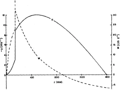
(2.37) - (2.39) may be solved numerically, given the radial profile vgr. We choose R = 500 km. Radial profiles of selected dynamical quantities in the boundary layer and at the top of it are shown in Fig. 2.5 for this calculation. At large radii (r > 350 km), the mean vertical motion at the top of the boundary layer,wδ, is downward and the total wind speed |vb| = p
u2b +v2b is less than that at the top of the boundary layer, vgr. As r decreases, both ub and vb increase in magnitude, as does vgr, the maximum value of vb occurring just inside the radius of maximum tangential wind speed (RMW) above the boundary layer. As a result, the frictional force, F = Cd|vb|vb/δ increases, and in particular its radial component, Fr, denoted by f ri in the top right panel of Fig 2.5. The net radially-inward pressure gradient force per unit mass, (vgr2 −v2b)/r+f(vgr−vb), denoted bypgf, increases also with decreasing r, at least for large r, but more rapidly than the frictional force. The reason is that columns of fluid partially conserve their absolute angular momentum as they converge in the boundary layer and despite some frictional loss to the surface, their rotation rate increases. The increase in vb is assisted by the downward transfer of tangential momentum from above, represented by the term (wδ−+wsc)(vb−vgr)/δin Eq. (2.38), although this effect turns out to be very small. The downward transfer of (zero) radial momentum, represented by the term (wδ−+wsc)ub/δ in Eq. (2.37), is denoted by wu in Fig. 2.5, but this also makes a negligible contribution to the force balance in the boundary layer. For the typical tangential wind profile used, vb increases faster than vgr as r decreases inside a radius of about 200 km. In this region, pgf decreases faster than wu+f ri so that eventually the net radial force pgf −wu−f ri changes sign. This change occurs well before the RMW is reached.
Whenpgf−wu−f ribecomes positive, the radial inflow decelerates, butvb continues to increase as columns of air continue to move inwards. Eventually, vb asymptotes tovgr and pgf tends to zero, but at no point does the tangential wind speed become supergradient. Nevertheless, as pgf tends to zero, the net outward force, primarily due to friction, becomes relatively large and the inflow decelerates very rapidly.
The mean vertical velocity at the top of the boundary layer increases steadily with decreasing rand reaches a maximum very close to the RMW: thereafter it decreases rapidly.
The lower right panel of Fig. 2.5 shows how the absolute angular momentum in the boundary layer decreases with decreasing radius as a result of the surface frictional torque. However, the rate of decrease is less rapid than that above the boundary layer and value in the boundary layer asymptotes to the value above the layer at inner radii.
It turns out that, except for a short adjustment length, which decreases in radial extent with increasing R, the calculations are relatively insensitive to the choice of R (see Smith, 2003). This insensitivity to R is not true of the thermodynamic fields
Figure 2.5: Radial profiles of selected dynamical quantities in the boundary layer calculation: (top left) tangential and radial components of wind speed in the bound- ary layer (ub, vb), total wind speed in the boundary layer, vv, and tangential wind speed above the boundary layer (vgr - the unmarked solid line) [Units m s−1]; (top, right) radial pressure gradient force (pgf) and frictional force (fri) per unit mass in the boundary layer, together with the force associated with the downward flux of radial momentum through the top of the boundary layer (wu) [Units 1.0×10⁻³ m s−2] and the sum of these three forces (solid line); (bottom left) vertical velocity at the top of the boundary layer, wδ [Units cm s−1]; (bottom right) absolute angular momentum above the boundary layer (solid line) and in the boundary layer (amb) [Units 1.0×10⁷ m2 s−2].
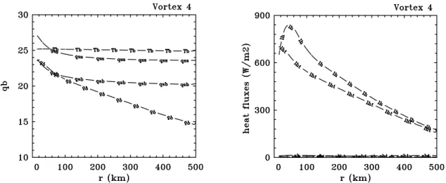
Figure 2.6: Radial profiles of selected thermodynamic quantities in the control calcu- lation: (left panel) boundary layer temperature (Tb, unit deg. C), specific humidity (qb), saturation specific humidity (qsb), and the saturation specific humidity at the sea surface (qss) [Units gm kg−1]; (right panel) latent heat fluxes from the sea surface (lh) and through the top of the boundary layer (lht)), and corresponding sensible heat fluxes (the two curves just above the abscissa labelled ”sh” and ”sht”) [Units W m−2].
as discussed below.
2.9.3 Thermodynamic aspects
The left panel of Fig. 2.6 shows the radial profiles of boundary layer temperature, specific humidity and saturation specific humidity, together with the saturation spe- cific humidity at the sea surface temperature (qss), while the right panel shows the fluxes of sensible and latent heat at the surface and through the top of the boundary layer. At large radii, the wind speed is comparatively light and the boundary layer is in approximate3 radiative-convective equilibrium. In particular, the air temperature just above the sea surface is only slightly lower than the sea surface temperature;
the net sensible heat fluxes from the sea and through the top of the boundary layer approximately balance the radiative cooling; and the moistening of the boundary layer by the surface flux approximately balances the drying brought about by subsi- dence associated with shallow convection. The mass flux of shallow convection and the boundary layer depth are chosen to ensure this balance.
As r decreases and the surface wind speed increases, the surface moisture flux increases and the boundary layer progressively moistens. The increase in moisture contrast between the boundary layer and the air aloft leads to an increase in the flux
3The radiative-convective state is very sensitive to the choice of parameters including the mass flux of shallow convection and the boundary layer depth. We choose rounded numbers for these quantities so that the boundary layer is close to, but not exactly in equilibrium.
of dry air through the top of the subcloud layer, which reduces the rate of moisten- ing. This effect would be reduced in a more complete model in which the moisture content above the boundary layer is predicted. If shallow convection and radiative cooling are omitted, the rate of moistening is relatively rapid and the boundary layer saturates (i.e. qb = qs at a relatively large radius (453 km), although, of course, then the boundary layer is not in radiative-convective equilibrium at r =R. In the present case, saturation occurs at a radius of about 80 km, but the air just above the sea surface does not (i.e. qb < qss), which in terms of the simple model could be interpreted to mean that the boundary layer becomes topped by low cloud. A further consequence is that the surface moisture fluxes do not shut off. We have not allowed for the latent heat release in the inner core in these calculations as the degree of supersaturation is only about 1% (see Smith, 2003, Fig. 11). The degree of mois- ture disequilibrium at the sea surface is maintained by the fact that the saturation specific humidity increases as the surface pressure decreases. The latent heat fluxes are much larger than the sensible heat fluxes.
2.10 Radiative cooling
The tropical atmosphere is stably stratified so that large vertical displacements of air parcels may only occur in the presence of diabatic processes: parcel ascent can occur over significant depths only if there is latent heat release to counter adiabatic cooling (i.e. if the ascent occurs in cloud); and parcel subsidence can occur over a substantial depth only if there is radiative cooling to counter adiabatic warming. Thus radiative effects in tropical cyclones cannot be ignored if we wish to understand the subsiding branch of the secondary circulation. The following discussion of radiative effects is based on that of Anthes (1979, p218-9).
Diabatic heating rates associated with the absorption of shortwave radiation en- ergy and the emission of longwave radiation are quite small compared with the heat- ing rates associated with condensation in deep precipitating clouds. In the cloud-free regions of the tropical atmosphere the mean radiative cooling rate is 1 to 2◦C/day from the surface to 10 km (≈250 mb) and decreases to about zero at the tropopause.
In a region of multi-layer clouds, however, there is practically no radiative cooling in the clouds, but there is strong cooling at their top.
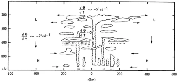
The result of differential radiative heating between the cloud-free environment and a cloudy tropical depression or tropical cyclone is to generate a direct circulation, with sinking motion in the clear air and rising motion in the cloudy air (Fig. 2.7). In the tropical cyclone, radiation acts to maintain the baroclinicity associated with the warm core. However, it is a smaller effect than differential heating by condensation, except possibly in lightly precipitating systems. This may be seen by relating the mean diabatic rate of temperature in a column of air of unit cross-section extending from 1000 mb to 100 mb to the rainfall rate Rf (cm/day):
∂T
∂t =−2.67Rf (oC/day). (2.47)
Figure 2.7: Schematic diagram of radiatively-induced circulation in a tropical distur- bance. In clear air surrounding the cloudy centre, diabatic cooling is about 2◦C/day.
In the cloudy interior, radiative cooling is nearly zero. The differential cooling in- duces sinking motion in the environment, where pressures rise at the surface and fall aloft. Flow in low levels is toward the centre of the disturbance, aloft it is outward.
(From Anthes, 1979)
For typical cloud cluster rainfall rates of 2.5 cm/day (Ruprecht and Gray, 1976), the average tropospheric rate of temperature change would be 6.7 cm/day, which is about five times larger than the effect of radiation. For hurricanes, a typical rainfall rate in the inner 222 km region is 9.5 cm/day, which gives ∂T /∂t = −25◦C/day, more than an order of magnitude larger than the radiative cooling rate. Thus, without latent heat release, only a slow meridional circulation could be maintained by radiation because the lifting of statically-stable air leads to cooling and a negative buoyancy force that opposes the circulation induced by radiative cooling. With latent heating, however, the mean adiabatic cooling in the ascending branch of the secondary circulation is opposed and much larger upward velocities may be attained.
When direct absorption of shortwave solar radiation is considered, a diurnal vari- ation of the radial differential cooling rate is introduced. The differential cooling during the day is reduced from a nocturnal value of 2◦C/day to a value of about 1◦C/day in the middle troposphere. For ∂T /∂p≈8◦C/(100 mb), ∂T /∂t≈1◦C/day corresponds to a vertical velocity ω of about 12.5 mb/day, which is supported by a mean divergence of 5×10⁻⁷ s−1 between the surface and 500 mb. This is much smaller than the observed diurnal variation in low-level divergence, which is about 5×10⁻⁶ s−1 (Gray and Jacobson, 1977). What probably happens is that the small diurnal variation in radiation-induced divergence triggers a much larger response by modulating deep cumulus convection. During the night, when differential cooling is at a maximum, upper-level divergence over the disturbance and low-level conver-
gence into the disturbance results in a dramatic increase in convection. After sunrise, absorption of solar radiation in the cloud-free environment and increased subsidence from the enhanced secondary circulation during the night reduces the mean temper- ature difference between the disturbance and its environment. The mean circulation then diminishes and the deep cumulus clouds weaken.
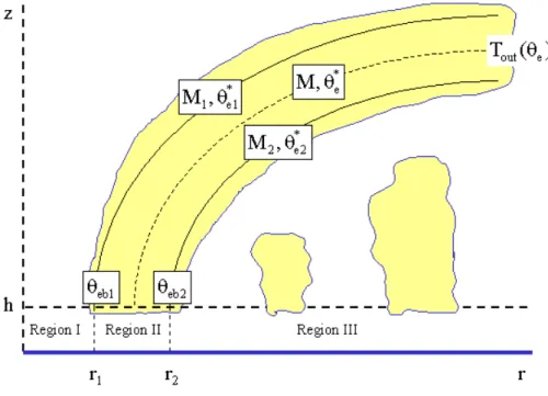
2.11 The Emanuel steady-state model
The basis of Emanuel’s steady-state model for a tropical cyclone, described by Emanuel (1986), is Fig. 2.4. It is convenient to divide the domain into three re- gions as shown in Fig. 2.8. Regions I and II encompass the eye and eyewall regions, respectively, while Region III refers to that beyond the eyewall clouds. Region II is where the upward mass flux at the top of the boundary layer is large compared with that associated with shallow convection. Smith (2003, p1013) estimated a value for wsc (defined in section 2.9.1) of about 2 cm s−1, based on the radiative equilibrium of the boundary layer at some large radius. In the boundary layer calculation shown in Fig. 2.5, w > 5wsc for r < 2rm, where rm is the radius of maximum tangential wind speed above the boundary layer. By comparison, Emanuel op. cit. takes the outer radius of Region II to be rm.
In pressure coordinates, the gradient wind equation and hydrostatic equation may be written as:
g µ∂z
∂r
p
= M2
r3 − 14rf2 (2.48)
and
g µ∂z
∂p
r
=−α, (2.49)
where α = 1/ρ is the specific volume. Eliminating the geopotential height of the pressure surface, gz, gives an alternative form of the thermal wind equation:
1 r3
µ∂M2
∂p
r
=− µ∂α
∂r
p
. (2.50)
At this point it is convenient to introduce the saturation moist entropy, s∗, defined by:
s∗ = lnθe∗, (2.51)
which is a state variable. Therefore we can regard α as a function of p and s∗ and with a little manipulation we can express the thermal wind equation as:
1 r3
µ∂M2
∂p
r
=− µ∂α
∂s∗
p
µ∂s∗
∂r
p
. (2.52)
I will show in an Appendix 2.16.1 that µ∂α
∂s∗
p
= µ∂T
∂p
s∗
, (2.53)
whereupon Eq. (2.52) becomes
Figure 2.8: Schematic diagram of the secondary circulation of a mature tropical cyclone showing the eye and the eyewall clouds. The absolute angular momentum per unit mass,M, and equivalent potential temperature,θeof an air parcel are conserved after the parcel leaves the boundary layer and ascends in the eyewall clouds. The precise values of these quantities depend on the radius at which the parcel exits the boundary layer. At radii beyond the eyewall cloud, shallow convection plays an important role in moistening and cooling the lower troposphere above the boundary layer and warming and drying the boundary layer as indicated.
1 r3
µ∂M2
∂p
r
=− µ∂T
∂p
s∗
µ∂s∗
∂r
p
. (2.54)
With the assumption that M and s∗ surfaces coincide, i.e. M =M(s∗), Eq. (2.54) becomes
2M r3
µ∂M
∂p
r
=− µ∂T
∂p
s∗
ds∗ dM
µ∂M
∂r
p
. (2.55)
Note that∂T /∂p)s∗ is just the temperature lapse rate as a function of pressure along a moist adiabat. Now along an M surface,
µ∂M
∂r
z
δr+ µ∂M
∂p
r
δp= 0, (2.56)