Flavour tagged time dependent angular analysis of the B 0

ATLAS-CONF-2013-039 12April2013

ATLAS NOTE

ATLAS-CONF-2013-039

April 9, 2013

Flavour tagged time dependent angular analysis of the B ⁰

_s

→ J/ψ φ decay and extraction of ∆Γ

s

and the weak phase φ

s

in ATLAS

The ATLAS Collaboration

Abstract

A measurement of the

B⁰_s→J/ψ φ

decay parameters, updated to include flavour tagging is reported using 4.9 fb

⁻¹

of integrated luminosity collected by the ATLAS detector from

pp

collisions recorded in 2011. The values measured for the physical parameters are:

φs=

0.12

±

0.25

(stat.)±

0.11

(syst.)

rad

∆Γs=

0.053

±

0.021

(stat.)±

0.009

(syst.)

ps

⁻¹

Γs=

0.677

±

0.007

(stat.)±

0.003

(syst.)

ps

⁻¹

|A₀(0)|²=

0.529

±

0.006(stat.)

±

0.011

(syst.)

|A_k(0)|²=

0.220

±

0.008(stat.)

±

0.009

(syst.) δ⊥=

3.89

±

0.46

(stat.)±

0.13

(syst.)

rad

where the parameter

∆Γs

is constrained to be positive. The fraction

|A_S(0)|²

, of

S-wave KK

or

f₀

contamination through the decays

B⁰_s →J/ψK⁺K⁻(f₀)

is also measured and is found to be compatible with zero. Results for

φs

and

∆Γs

are also presented as 68% and 95%

likelihood contours, which show agreement with the Standard Model expectations.

c Copyright 2013 CERN for the benefit of the ATLAS Collaboration.

Reproduction of this article or parts of it is allowed as specified in the CC-BY-3.0 license.

1 Introduction

New phenomena beyond the predictions of the Standard Model (SM) may alter CP violation in B-decays.

A channel that is expected to be sensitive to new physics contributions is the decay B

⁰_s →

J/ψ φ . CP violation in the B

⁰_s→

J/ψ φ decay occurs due to interference between direct decays and decays occurring through B

⁰_s−

B

⁰_s

mixing. The oscillation frequency of B

⁰_s

meson mixing is characterized by the mass difference

∆ms

of the heavy (B

H

) and light (B

L

) mass eigenstates. The CP-violating phase

φs

is defined as the weak phase difference between the B

⁰_s−

B

⁰_s

mixing amplitude and the b

→

ccs decay amplitude. In the absence of CP violation, the B

_H

state would correspond exactly to the CP-odd state and the B

_L

to the CP-even state. In the SM the phase

φs

is small and can be related to CKM quark mixing matrix elements via the relation

φs' −2βs

, with

βs=

arg[−(V

ts

V

_tb^∗)/(Vcs

V

_cb^∗)]; a value ofφs' −2βs=−0.0368±

0.0018 rad [1] is predicted in the SM. Many new physics models predict large

φs

values whilst satisfying all existing constraints, including the precisely measured value of

∆ms

[2, 3].

Another physical quantity involved in B

⁰_s−

B

⁰_s

mixing is the width difference

∆Γs=ΓL−ΓH

of B

L

and B

_H

which is predicted to be

∆Γs=

0.087

±

0.021 ps

⁻¹

[4]. Physics beyond the SM is not expected to affect

∆Γs

as significantly as

φs

[5]. Extracting

∆Γs

from data is nevertheless useful as it allows theoretical predictions to be tested [5].

The decay of the pseudoscalar B

⁰_s

to the vector-vector final-state J/ψ φ results in an admixture of CP-odd and CP-even states, with orbital angular momentum L

=

0, 1 or 2. The final states with orbital angular momentum L

=

0 or 2 are CP-even while the state with L

=

1 is CP-odd. Flavour tagging is used to distinguish between the initial B

⁰_s

and B

⁰_s

states. The CP states are separated statistically through the time-dependence of the decay and angular correlations amongst the final-state particles.

In this paper, an update to the previous measurement [6] of

φs

, the average decay width

Γs = (ΓL+ΓH)/2 and the value of∆Γs

, using flavour tagging, is presented. Previous measurements of these quantities have been reported by the CDF and DØ collaborations [7, 8] and recently by the LHCb col- laboration [9]. The analysis presented here uses LHC pp data at

√

s

=

7 TeV collected by the ATLAS detector in 2011.

2 ATLAS detector and Monte Carlo simulation

The ATLAS experiment [10] is a multipurpose particle physics detector with a forward-backward sym- metric cylindrical geometry and near 4π coverage in solid angle. The inner tracking detector (ID) con- sists of a silicon pixel detector, a silicon microstrip detector and a transition radiation tracker. The ID is surrounded by a thin superconducting solenoid providing a 2 T axial magnetic field, and by an high- granularity liquid-argon (LAr) sampling electromagnetic calorimeter. An iron/scintillator tile calorimeter provides hadronic coverage in the central rapidity range. The end-cap and forward regions are instru- mented with LAr calorimeters for both electromagnetic and hadronic measurements. The muon spec- trometer (MS) surrounds the calorimeters and consists of three large superconducting toroids with eight coils each, a system of tracking chambers, and detectors for triggering.

The muon and tracking systems are of particular importance in the reconstruction of B meson candi- dates. Only data where both systems were operating correctly and where the LHC beams were declared to be stable are used. A muon identified using a reconstruction relying on a statistical combination of MS and ID track parameters is referred to as combined. A muon formed by segments which are not associated with an MS track, but which are matched to ID tracks extrapolated to the MS is referred to as segment tagged.

The data were collected during a period of rising instantaneous luminosity at the LHC, and the

trigger conditions varied over this time. The triggers used to select events for this analysis are based on

identification of a J/ψ

→µ⁺µ⁻

decay, with either a 4 GeV transverse momentum

^∗

(p

T

) threshold for each muon or an asymmetric configuration that applies a p

_T

threshold beyond 4 GeV p

_T

to one of the muons and accepting the second muon with p

_T

as low as 2 GeV.

Monte Carlo (MC) simulation is used to study the detector response, estimate backgrounds and model systematic effects. For this study, 12 million MC-simulated B

⁰_s→

J/ψ φ events were generated using PYTHIA [11] tuned with recent ATLAS data [12]. No p

_T

cuts were applied at the generator level. Detector responses for these events were simulated using the ATLAS simulation package based on GEANT4 [13]. In order to take into account the varying trigger configurations during data-taking, the MC events were weighted to have the same trigger composition as the collected collision data. Additional samples of the background decay B

⁰_d→

J/ψK

^0∗

as well as the more general bb

→

J/ψ X and pp

→

J/ψ X backgrounds were also simulated using PYTHIA.

3 Reconstruction and candidate selection

Events passing the trigger and the data quality selections described in Section 2 are required to pass the following additional criteria: the event must contain at least one reconstructed primary vertex built from at least four ID tracks and at least one pair of oppositely charged muon candidates that are reconstructed using one of the two algorithms that combine the information from the MS and the ID [14]. In this analysis the muon track parameters are taken from the ID measurement alone, since the precision of the measured track parameters for muons in the p

_T

range of interest for this analysis is dominated by the ID track reconstruction. The pairs of muon tracks are refitted to a common vertex and accepted for further consideration if the fit results in

χ²

/d.o.f.

<

10. The invariant mass of the muon pair is calculated from the refitted track parameters. To account for varying mass resolution, the J/ψ candidates are divided into three subsets according to the pseudorapidity

η

of the muons. A maximum likelihood fit is used to extract the J/ψ mass and the corresponding resolution for these three subsets. When both muons have

|η|<

1.05, the di-muon invariant mass must fall in the range

(2.959−

3.229) GeV to be accepted as a J/ψ candidate. When one muon has 1.05

<|η|<

2.5 and the other muon

|η|<

1.05, the corresponding signal region is

(2.913−

3.273) GeV. For the third subset, where both muons have 1.05

<|η|<

2.5, the signal region is

(2.852−

3.332) GeV. In each case the signal region is defined so as to retain 99.8% of the J/ψ candidates identified in the fits.

The candidates for

φ→

K

⁺

K

⁻

are reconstructed from all pairs of oppositely charged particles with p

_T>

0.5 GeV and

|η|<

2.5 that are not identified as muons. Candidates for B

⁰_s→

J/ψ

(µ⁺µ⁻)φ(K⁺

K

⁻)

are sought by fitting the tracks for each combination of J/ψ

→µ⁺µ⁻

and

φ →

K

⁺

K

⁻

to a common vertex. Each of the four tracks are required to have at least one hit in the pixel detector and at least four hits in the silicon strip detector. The fit is further constrained by fixing the invariant mass calculated from the two muon tracks to the world average J/ψ mass [15]. These quadruplets of tracks are accepted for further analysis if the vertex fit has a

χ²

/d.o.f.

<

3, the fitted p

_T

of each track from

φ →

K

⁺

K

⁻

is greater than 1 GeV and the invariant mass of the track pairs (under the assumption that they are kaons) falls within the interval 1.0085 GeV

<

m(K

⁺

K

⁻)<

1.0305 GeV. In total 131k B

⁰_s

candidates are collected within a mass range of 5.15

<

m(B

⁰_s)<

5.65 GeV used in the fit.

For each B

⁰_s

meson candidate the proper decay time t is determined by the expression:

t

=

L

_xy

M

_B

c p

_TB ,

where p

_TB

is the reconstructed transverse momentum of the B

⁰_s

meson candidate and M

_B

denotes the world average mass value [15] of the B

⁰_s

meson (5.3663 GeV). The transverse decay length, L

_xy

, is the

∗The ATLAS coordinate system and the definition of transverse momentum are described in reference [10]

displacement in the transverse plane of the B

⁰_s

meson decay vertex with respect to the primary vertex, projected onto the direction of the B

⁰_s

transverse momentum. The position of the primary vertex used to calculate this quantity is refitted following the removal of the tracks used to reconstruct the B

⁰_s

meson candidate.

For the selected events the average number of pileup interactions is 5.6, necessitating a choice of the best candidate for the primary vertex at which the B

⁰_s

meson is produced. The variable used is a three-dimensional impact parameter d

₀

, which is calculated as the distance between the line extrapolated from the reconstructed B

⁰_s

meson vertex in the direction of the B

⁰_s

momentum, and each primary vertex candidate. The chosen primary vertex is the one with the smallest d

₀

. Using MC simulation it is shown that the fraction of B

⁰_s

candidates which are assigned the wrong primary vertex is less than 1% and that the corresponding effect on the final results is negligible. No B

⁰_s

meson lifetime cut is applied in the analysis.

4 Flavour tagging

The determination of the initial flavour of neutral B-mesons can be inferred using information from the other B-meson that is typically produced from the other b quark in the event, referred to as the Opposite- Side Tagging (OST).

To study and calibrate the OST methods, the decays of B

^±→

J/ψ K

^±

can be used, where flavour of the charge of the B-meson at production is provided by the kaon charge. Events from the entire 2011 run period satisfying the same data quality selections as described in section 2 are used.

4.1 B

^±

→ J/ψ K

^±

event selection

To be selected for use in the calibration analysis, events must satisfy a trigger condition requiring two oppositely-charged muons within an invariant mass range around the nominal J/ψ mass. Candidate B

^± →

J/ψK

^±

decays are identified using two oppositely-charged combined muons forming a good vertex using information supplied by the inner detector. Each muon is required to have a transverse momentum of at least 4 GeV and pseudo-rapidity within

|η|<

2.5. The invariant mass of the di-muon candidate is required to satisfy 2.8

<

m(µ µ)

<

3.4 GeV. To form the B candidate an additional track with p

_T>

1 GeV ,

|η|<

2.5 is combined with the di-muon candidate and a vertex fit performed applying a mass-constraint for the di-muons to the known value of the J/ψ mass. To reduce the majority of the prompt component of the combinatorial background the requirement L

xy>

0.1 mm is made on the B candidate.

In order to study the distributions corresponding to the signal processes with the background com- ponent removed, a sideband subtraction method is defined. Events are separated into five regions of B candidate rapidity and three mass regions. The mass regions are defined as a signal region around the fitted peak signal mass position

µ±

2σ and the sidebands are

[µ−

5σ

,µ−

3σ

]

and

[µ+

3σ

,µ+

5σ

],

where

µ

and

σ

are the peak and widths of the Gaussian model of the B signal mass respectively. Indi- vidual binned extended likelihood fits are performed to the invariant mass distribution in each region of rapidity.

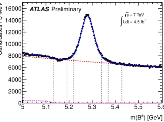
The background is modelled by an exponential to describe combinatorial background and a hyper-

bolic tangent function to parameterise the low-mass contribution from mis- and partially-reconstructed

B decays. This component has negligible contribution to either the signal or sideband regions. Figure 1

shows the invariant mass distribution of B candidates for all rapidity regions overlaid with the fit result

for the combined data.

) [GeV]

m(B±

5 5.1 5.2 5.3 5.4 5.5 5.6

Candidates / 3 MeV

0 2000 4000 6000 8000 10000 12000 14000 16000

Ldt = 4.5 fb-1

∫ ^{s = 7 TeV}

ATLASPreliminary

Figure 1: The invariant mass distribution for B

^±→

J/ψ K

^±

candidates. Included in this plot are all events passing the selection criteria. The data are shown by points, the overall result of the fit is given by the blue curve. The combinatorial background component is given by the dashed line, and the contribution of the background from partially reconstructed decays is shown in the dotted curve. The red vertical dashed lines indicate the left and right sidebands while the blue vertical dashed lines indicate the signal region.

4.2 Tagging methods

Several methods are available to infer the flavour of the opposite-side meson, with varying efficiencies and discriminating powers. Identifying the charge of a muon through the semi-leptonic decay of the B meson provides strong power of separation, however the b

→µ

transitions are diluted through neutral B meson oscillations, as well as by cascade decays b

→

c

→µ

which can alter the sign of the muon relative to the one coming from direct semi-leptonic decays b

→µ

. The separation power of tag muons can be enhanced by considering a weighted sum of the charge of the tracks in a cone around the muon. If no muon is present, a weighted sum of the charge of tracks associated to the opposite side B meson decay will also provide some separation. The tagging methods are described in detail below.

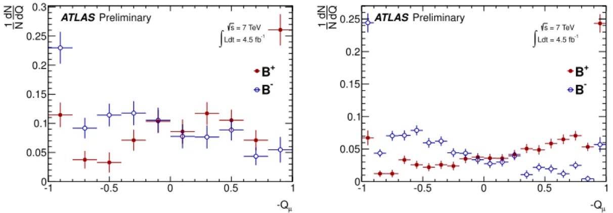
An additional muon is searched for in the event, having originated near the original interaction point.

Muons are separated into their two reconstruction classes: combined and segment tagged. In the case of multiple muons, the one with the highest transverse momentum is selected. A muon cone charge variable is constructed, defined as

Q

_µ=∑^Ni ^tracks

q

ⁱ·(pⁱ_T)^κ

∑^Ni ^tracks(

p

ⁱ_T)^κ ,

(1)

where the value of the parameter

κ=

1.1, which was tuned to optimise the tagging power, and the sum is performed over the reconstructed ID tracks within a cone of

∆R<

0.5 around the muon momentum axis, with p

_T>

0.5 GeV and

|η|<

2.5. The value of parameter

κ

has been determined in the process of optimisation of the tagging performance. Tracks associated to the signal-side of the decay are explicitly excluded from the sum. In Fig. 2 the distribution of muon cone charge is shown for candidates from B

^±

signal decays, for each class of muon.

In the absence of a muon, a b-tagged jet [16] is required in the event, with tracks associated to the

same primary interaction vertex as the signal decay, excluding those from the signal candidate. The jet is

reconstucted using the Anti-k

t

algorithm with a cone size of 0.6. In the case of multiple jets, the jet with

the highest value of the b-tag weight reference is used.

-Qµ

-1 -0.5 0 0.5 1

dQdN

N1

0 0.05 0.1 0.15 0.2 0.25 0.3

B+

B- Ldt = 4.5 fb-1

∫ ^{s = 7 TeV}

ATLASPreliminary

-Qµ

-1 -0.5 0 0.5 1

dQdN

N1

0 0.05 0.1 0.15 0.2 0.25

B+

B- Ldt = 4.5 fb-1

∫ ^{s = 7 TeV}

ATLASPreliminary

Figure 2: Muon cone charge distribution for B

^±

signal candidates for segment tagged (left) and combined (right) muons.

A jet charge is defined

Q

_jet=∑^Ni ^tracks

q

ⁱ·(pⁱ_T)^κ

∑^Ni ^tracks(

p

ⁱ_T)^κ ,

(2)

where

κ=

1.1, and the sum is over the tracks associated to the jet, using the method described in [17].

Figure 3 shows the distribution of charges for jet-charge from B

^±

signal-side candidates.

-Qjet

-1 -0.5 0 0.5 1

dQdN

N1

0 0.02 0.04 0.06 0.08 0.1 0.12 0.14 0.16 0.18

B+

B- Ldt = 4.5 fb-1

∫ ^{s = 7 TeV}

ATLASPreliminary

Figure 3: Jet-charge distribution for B

^±

signal candidates.

The efficiency

ε

of an individual tagger is defined as the ratio of the number of tagged events to the total number of candidates. A probability that a specific event has a signal decay containing a ¯ b given the value of the discriminating variable P(B|Q) is constructed from the calibration samples for each of the B

⁺

and B

⁻

samples, defining P(Q|B

⁺)

and P(Q|B

⁻)

respectively. The probability to tag a signal event as a ¯ b is therefore P(B|Q) = P(Q|B

⁺)/(P(Q|B⁺) +

P(Q|B

⁻))

and P( B|Q) = ¯ 1

−

P(B|Q). The tagging power is defined as

εD²=∑iεi·(2Pi(B|Qi)−

1)

²

, where the sum is over the bins of the probability distribution as a function of the charge variable. An effective dilution

D

is calculated from the tagging power and the efficiency.

The combination of the tagging methods is applied according to the hierarchy of performance. The

single best performing tagging measurement is taken, according to the order: combined muon cone

charge, segment tagged muon cone charge, jet charge. If it is not possible to provide a tagging response

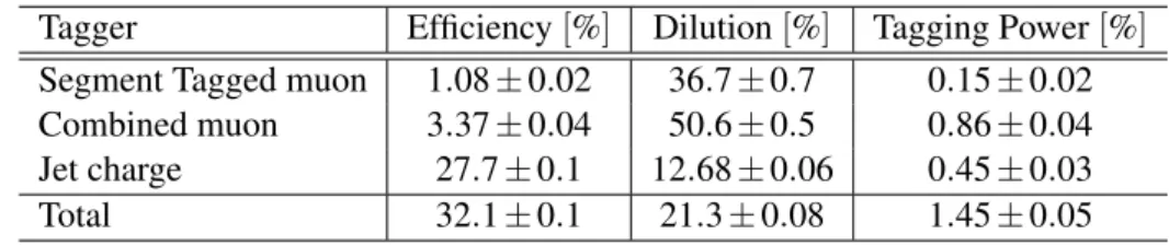
for the event, then the probability of 0.5 is assigned. A summary of the tagging performance is given in Table 1.

Table 1: Summary of tagging performance for the different tagging methods described in the text. Un- certainties shown are statistical only. The efficiency and tagging power are each determined by summing over the individual bins of the charge distribution. The effective dilution is obtained from the measured efficiency and tagging power, as shown in the table. For the efficiency, dilution, and tagging power, the corresponding uncertainty is each determined by combining the appropriate uncertainties on the individ- ual bins of each charge distribution.

Tagger Efficiency

[%]

Dilution

[%]

Tagging Power

[%]

Segment Tagged muon 1.08

±

0.02 36.7

±

0.7 0.15

±

0.02 Combined muon 3.37

±

0.04 50.6

±

0.5 0.86

±

0.04

Jet charge 27.7

±

0.1 12.68

±

0.06 0.45

±

0.03

Total 32.1

±

0.1 21.3

±

0.08 1.45

±

0.05

5 Maximum Likelihood Fit

An unbinned maximum likelihood fit is performed on the selected events to extract the parameters of the B

⁰_s →

J/ψ(µ

⁺µ⁻)φ(K⁺

K

⁻)

decay. The fit uses information about the reconstructed mass m, the measured proper decay time t, the measured mass and proper decay time uncertainties

σm

and

σt

, the tag probability, and the transversity angles

Ω

of each B

⁰_s →

J/ψ φ decay candidate. There are three transversity angles;

Ω= (θT,ψT,φT)

and these are defined in section 5.1.

The likelihood function is defined as a combination of the signal and background probability density functions as follows:

ln

L =

N i=1

∑

{wi·

ln( f

_s·Fs(mi,ti,Ωi) +

f

_s·

f

_B0·FB⁰(mi,ti,Ωi) +(1−

f

_s·(1+

f

_B0))Fbkg(mi,ti,Ωi))}

(3) where N is the number of selected candidates, w

i

is a weighting factor to account for the trigger effi- ciency, f

_s

is the fraction of signal candidates, f

_B0

is the fraction of peaking B

⁰

meson background events calculated relative to the number of signal events; this parameter is fixed in the likelihood fit. The mass m

_i

, the proper decay time t

_i

and the decay angles

Ωi

are the values measured from the data for each event i.

Fs

,

FB⁰

and

Fbkg

are the probability density functions (PDF) modelling the signal, the spe- cific B

⁰

background and the other background distributions, respectively. A detailed description of the signal PDF terms in equation 3 is given in sections 5.1. The terms describing the background PDFs are described in the previous analysis [6] and are unchanged.

5.1 Signal PDF

The PDF describing the signal events,

Fs

, has the form of a product of PDFs for each quantity measured from the data:

Fs(mi,ti,Ωi,P(B|Q)) =

P

_s(mi|σ_mi)·P_s(σm_i)·P_s(Ωi,ti,P(B|Q)|σ_ti)·P_s(σt_i)·P_s(P(B|Q))·A(Ω_i,

p

_Ti)·P_s(p_Ti)

(4)

The terms P

_s(mi|σm_i),

P

_s(Ωi,ti,P(B|Q)|σt_i)

and A(Ω

i,pTi)

are explained in the current section. The tagging probability term P

_s(P(B|Q))

is described in section 5.2 and the remaining probability terms P

_s(σm_i),

P

_s(σt_i)

and P

_s(p_Ti)

are unchanged from the previous analysis and described there [6]. Ignoring detector effects, the joint distribution for the decay time t and the transversity angles

Ω

for the B

⁰_s →

J/ψ(µ

⁺µ⁻)φ(K⁺

K

⁻)

decay is given by the differential decay rate [18]:

d

⁴Γ

dt dΩ

=

10

∑

k=1

O^(k)(t)g^(k)(θT,ψT,φT),

(5)

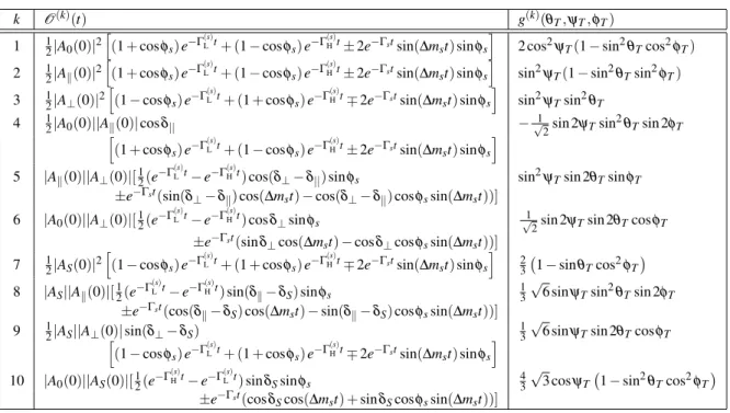
where

O^(k)(t)

are the time-dependent amplitudes and g

^(k)(θT,ψT,φT)

are the angular functions, given in table 2. The formulae for the time-dependent amplitudes have the same structure for B

⁰_s

and B

⁰_s

but with a sign reversal in the terms containing

∆ms

. A

⊥(t)

describes a CP-odd final-state configuration while both A

₀(t)

and A

_k(t)

correspond to CP-even final-state configurations. A

S

describes the contribution of CP-odd B

_s →

J/ψ K

⁺

K

⁻(

f

₀), where the non-resonant

KK or f

₀

meson is an S-wave state. The corresponding amplitudes are given in the last four lines of Table 2 (k=7-10) and follow the convention used in the previous analysis [9]. The likelihood is independent of the invariant KK mass distribution.

The equations are normalised such that the squares of the amplitudes sum to unity; three of the four amplitudes are fit parameters and

|A_⊥(0)|²

is determined according to this constraint.

The angles (θ

T,ψT,φT

), are defined in the rest frames of the final-state particles. The x-axis is determined by the direction of the

φ

meson in the J/ψ rest frame, the K

⁺

K

⁻

system defines the xy plane, where p

y(K⁺)>

0. The three angles are defined:

• θT

, the angle between p(µ

⁺)

and the xy plane, in the J/ψ meson rest frame

• φT

, the angle between the x-axis and p

_xy(µ⁺), the projection of theµ⁺

momentum in the xy plane, in the J/ψ meson rest frame

• ψT

, the angle between p(K

⁺)

and

−p(J/ψ)

in the

φ

meson rest frame

The signal PDF, P

s(Ω,t|σt)

needs to take into account lifetime resolution so each time element in Table 2 is smeared with a Gaussian function. This smearing is done numerically on an event-by-event basis where the width of the Gaussian is the proper decay time uncertainty, measured for each event, multiplied by a scale factor to account for any mis-measurements.

The angular sculpting of the detector and kinematic cuts on the angular distributions is included in the likelihood function through A(Ω

i,

p

Ti). This is calculated using a 4-D binned acceptance method,

applying an event-by-event efficiency according to the transversity angles (θ

T,ψT,φT

) and the p

_T

of the event. The p

_T

binning is necessary because the angular sculpting is influenced by the p

_T

of the B

⁰_s

. The acceptance was calculated from the B

⁰_s →

J/ψ φ MC events. In the likelihood function, the acceptance is treated as an angular sculpting PDF, which is multiplied with the the time and angular dependent PDF describing the B

⁰_s →

J/ψ

(µ⁺µ⁻)φ(K⁺

K

⁻)

decays, thus the complete angular function must be normalised simultaneously as both the acceptance and time-angular decay PDFs depend on the transversity angles. This normalisation is done numerically during the likelihood fit.

The signal mass function, P

_s(m), is modelled using a single Gaussian function smeared with an

event-by-event mass resolution. The PDF is normalised over the range 5150

<

M(B

⁰_s)<

5650 MeV.

5.2 Using tag information in the fit

The tag-probability for each B

⁰_s

candidate is determined from the calibrations of B

^±→

J/ψ K

^±

candi-

dates, as described in Section 4. The distributions of tag probabilities for the signal and background are

different and since the background cannot be factorized out, extra PDF terms are included to account for

Table 2: Table showing the ten time-dependent amplitudes,

O^(k)(t)

and the functions of the transversity angles g

^(k)(θT,ψT,φT). The amplitudes|A₀(0)|²

and

|Ak(0)|²

are for the CP even components of the B

⁰_s →

J/ψ φ decay,

|A(0)_⊥|²

is the CP odd amplitude, they have corresponding strong phases

δ₀

,

δ_k

and

δ⊥

, by convention

δ0

is set to be zero. The S−wave amplitude

|AS(0)|²

gives the fraction of B

⁰_s→

J/ψK

⁺

K

⁻(

f

₀)

and has a related strong phase

δS

. The

±

and

∓

terms denote two cases: the upper sign describes the decay of a meson that was initially a B

⁰_s

, while the lower sign describes the decays of a meson that was initially B

⁰_s

.

k O^(k)(t) g^(k)(θT,ψT,φT)

1 ¹₂|A₀(0)|²h

(1+cosφs)e^−Γ(s)Lt+ (1−cosφs)e^−Γ(s)Ht±2e^−Γstsin(∆mst)sinφs

i

2 cos²ψT(1−sin²θTcos²φT) 2 ¹₂|A_k(0)|²h

(1+cosφs)e^−Γ(s)Lt+ (1−cosφs)e^−Γ(s)Ht±2e^−Γstsin(∆mst)sinφs

i

sin²ψT(1−sin²θTsin²φT) 3 ¹₂|A_⊥(0)|²h

(1−cosφs)e^−Γ(s)Lt+ (1+cosφs)e^−Γ(s)Ht∓2e^−Γstsin(∆m_st)sinφs

i

sin²ψTsin²θT

4 ¹₂|A0(0)||A_k(0)|cosδ_|| −^√1

2sin 2ψTsin²θTsin 2φT

h

(1+cosφs)e^−Γ(s)Lt+ (1−cosφs)e^−Γ(s)Ht±2e^−Γstsin(∆mst)sinφs

i

5 |A_k(0)||A_⊥(0)|[¹₂(e^−Γ(s)Lt−e^−Γ(s)Ht)cos(δ_⊥−δ_||)sinφs sin²ψTsin 2θTsinφT

±e^−Γst(sin(δ_⊥−δ_k)cos(∆mst)−cos(δ_⊥−δ_k)cosφssin(∆mst))]

6 |A0(0)||A_⊥(0)|[¹₂(e^−Γ(s)Lt−e^−Γ(s)Ht)cosδ_⊥sinφs √1

2sin 2ψTsin 2θTcosφT

±e^−Γst(sinδ_⊥cos(∆mst)−cosδ_⊥cosφssin(∆mst))]

7 ¹₂|A_S(0)|²h

(1−cosφs)e^−Γ(s)Lt+ (1+cosφs)e^−Γ(s)Ht∓2e^−Γstsin(∆mst)sinφs

i 2

3 1−sinθTcos²φT 8 |AS||A_k(0)|[¹₂(e^−Γ(s)Lt−e^−Γ(s)Ht)sin(δ_k−δS)sinφs 1

3

√

6 sinψTsin²θTsin 2φT

±e^−Γst(cos(δ_k−δS)cos(∆mst)−sin(δ_k−δS)cosφssin(∆mst))]

9 ¹₂|A_S||A_⊥(0)|sin(δ_⊥−δS) ¹₃√

6 sinψTsin 2θ_Tcosφ_T h

(1−cosφs)e^−Γ(s)Lt+ (1+cosφs)e^−Γ(s)Ht∓2e^−Γstsin(∆mst)sinφs

i

10 |A0(0)||A_S(0)|[¹₂(e^−Γ(s)Ht−e^−Γ(s)Lt)sinδ_Ssinφs 4 3

√3 cosψT 1−sin²θTcos²φT

±e^−Γst(cosδScos(∆mst) +sinδScosφssin(∆mst))]

this difference. The distributions of the B

s

candidates tag-probabilities consist of continuous and discrete parts (spikes). These are described separately.

To describe the continuous parts, the sidebands are parametrized first. Sidebands are selected accord- ing to B

s

mass, i.e. m(B

s)<

5317 MeV or m(B

s)>

5417 MeV. In the next step, the same function as for the sidebands is used to describe events in the signal region: background parameters are fixed to the values obtained in sidebands while signal parameters are free in this step. The ratio of background and signal (obtained from simultaneous mass-lifetime fit) is fixed as well. The function describing tagging using combined muons has the form of a fourth-order Chebychev polynomial:

f

₁(x) =

1

+

∑

i=1,4

a

i

T

i(x)

(6)

for the tagging method using segment tagged muons a third order polynomial is used:

f

₂(x) =

1

+

∑

i=1,3

a

_i

x

ⁱ

(7)

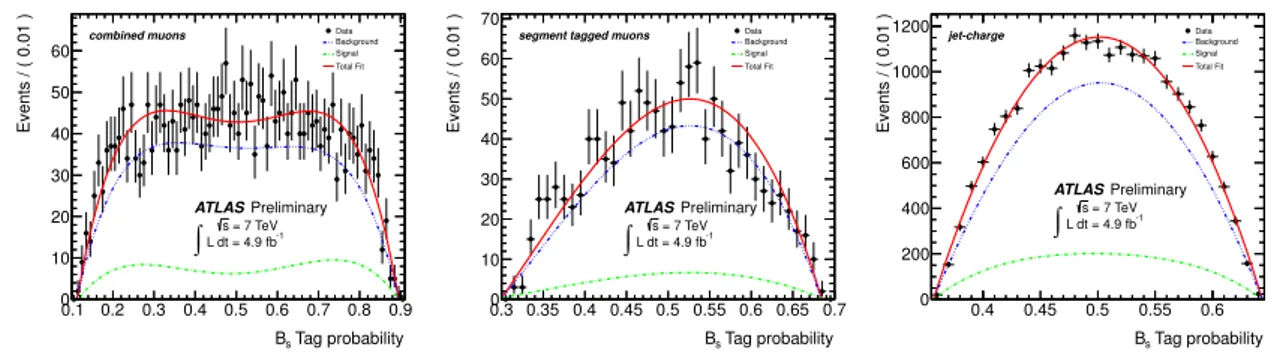
In both of the above formulas x represents the tag probability. A fourth-order Chebychev polynomial is also applied for the jet-charge tagging algorithm. In all three cases unbinned maximum likelihood fits are used. Results of fits projected on histograms are shown in Fig. 4.

Tag probability Bs

0.1 0.2 0.3 0.4 0.5 0.6 0.7 0.8 0.9

Events / ( 0.01 )

0 10 20 30 40 50 60

combined muons Data

Background Signal Total Fit

ATLASPreliminary L dt = 4.9 fb-1

∫ ^{s = 7 TeV}

Tag probability Bs

0.3 0.35 0.4 0.45 0.5 0.55 0.6 0.65 0.7

Events / ( 0.01 )

0 10 20 30 40 50 60 70

segment tagged muons ^Data_Background Signal Total Fit

ATLASPreliminary L dt = 4.9 fb-1

∫ ^{s = 7 TeV}

Tag probability Bs

0.4 0.45 0.5 0.55 0.6

Events / ( 0.01 )

0 200 400 600 800 1000

1200 _jet-charge Data

Background Signal Total Fit

ATLASPreliminary L dt = 4.9 fb-1

∫ ^{s = 7 TeV}

Figure 4: The tag probability for tagging using combined muons (left), segment tagged muons (middle) and jet-charge (right). Black dots are data after removing spikes, blue is a fit to the sidebands, green to the signal and red is a sum of both fits.

The spikes have their origin in tagging objects formed from a single track, providing a tag charge of exactly +1 or -1. When a background candidate is formed from a random combination of a J/ψ and a pair of tracks, the positive and negative charges are equally probable. However some of the background events are formed of partially reconstructed B-hadrons in these cases tag charges +1 or -1 are not equally probable. For signal events obviously tag charges are not symmetric. For the fit it is important to derive fractions f

₊₁

, f

₋₁

of events tagged with charges +1 and -1, respectively and separately for signal and background. The remaining 1- f

₊₁

- f

₋₁

is the fraction of events in continuous region. The fractions f

₊₁

and f

−1

are determined using the same B

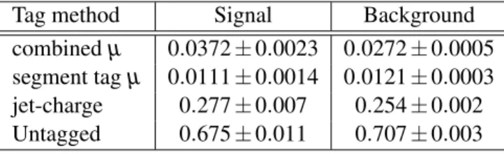
⁰_s

mass sidebands and signals regions as in case of continuous parts. Table 3 summarises the obtained relative probabilities between tag charges +1 and -1 for signal and background events and for all tag-methods. Similarly the sidebands subtraction method is also used to determine the relative population of the tag-methods in the background and signal events which also have to be included in the PDF. The results are summarised in Table 4.

If the tag-probability PDFs were ignored from the likelihood fit, equivalent to assuming identical

signal and background behaviour, the impact on the fit result would be small, affecting the results by less

then 10% of the statistical uncertainty.

Table 3: Table summarising the obtained relative probabilities between tag charges +1 and -1 for signal and background events and for all tag-methods. Only statistical errors are quoted. The asymmetry in the signal combined-muon tagging method has no impact on the results as it affects only 1% of the signal events (in addition to the negligible effect of the tag-probability distributions themselves).

Tag method Signal Background

f

₊₁

f

−1

f

₊₁

f

−1

combined

µ

0.106

±

0.019 0.187

±

0.022 0.098

±

0.006 0.108

±

0.006 segment tag

µ

0.152± 0.043 0.153

±

0.043 0.098

±

0.009 0.095± 0.008 jet-charge 0.167± 0.010 0.164

±

0.010 0.176

±

0.003 0.180± 0.003

Table 4: Table summarising the relative population of the tag-methods in the background and signal events. Only statistical errors are quoted.

Tag method Signal Background

combined

µ

0.0372

±

0.0023 0.0272

±

0.0005 segment tag

µ

0.0111

±

0.0014 0.0121

±

0.0003 jet-charge 0.277

±

0.007 0.254

±

0.002 Untagged 0.675

±

0.011 0.707

±

0.003

6 Results

The full simultaneous maximum likelihood fit contains 25 free parameters. This includes the nine physics parameters:

∆Γs

,

φs

,

Γs

,

|A₀(0)|²

,

|A_k(0)|²

,

δ||

,

δ⊥

,

|A_S|²

and

δS

. The other parameters in the likelihood function are the B

⁰_s

signal fraction f

_s

, the parameters describing the J/ψ φ mass distribution, the parame- ters describing the B

⁰_s

meson decay time plus angular distributions of background events, the parameters used to describe the estimated decay time uncertainty distributions for signal and background events, and scale factors between the estimated decay time and mass uncertainties and their true uncertainties. In ad- dition to this there are also 82 nuisance parameters describing the background and acceptance functions that are fixed at the time of the fit.

The number of signal B

⁰_s

meson candidates extracted from the fits is 22670

±

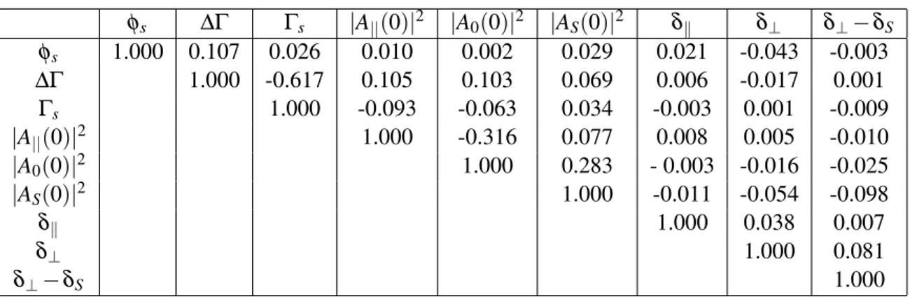
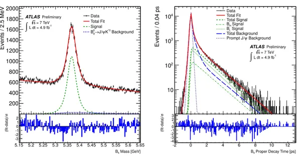
150. The results and correlations for the measured physics parameters of the simultaneous unbinned maximum likelihood fit are given in Table 5 and 6. Fit projections of the mass, proper decay time and angles are given in Figures 5 and 6 respectively.

7 Systematic uncertainties

Systematic uncertainties are assigned by considering several effects that are not accounted for in the likelihood fit. These are described below.

• Inner Detector Alignment:

Residual misalignments of the Inner Detector will affect the impact

parameter distribution with respect to the primary vertex. The impact of the residual misalignment

is estimated using simulated events with and without distorted geometry. For this the impact

parameter distribution with respect to the primary vertex is measured with data as a function of

η

and

φ

with the maximum deviation from zero being less than 10

µ

m. The measurement is used to

distort the geometry for simulated events in order to reproduce the impact parameter distribution

Table 5: Fitted values for the physical parameters along with their statistical and systematic uncertainties.

Parameter Value Statistical Systematic uncertainty uncertainty

φs

(rad) 0.12 0.25 0.11

∆Γs

(ps

⁻¹

) 0.053 0.021 0.009

Γs

(ps

⁻¹

) 0.677 0.007 0.003

|A_k(0)|²

0.220 0.008 0.009

|A₀(0)|²

0.529 0.006 0.011

|A_S|²

0.024 0.014 0.028

δ⊥

3.89 0.46 0.13

δ_k

[3.04-3.23] 0.09

δ⊥−δS

[3.02-3.25] 0.04

Table 6: Correlations between the physics parameters.

φs ∆Γ Γs |A_||(0)|² |A₀(0)|² |A_S(0)|² δk δ⊥ δ⊥−δS

φs

1.000 0.107 0.026 0.010 0.002 0.029 0.021 -0.043 -0.003

∆Γ

1.000 -0.617 0.105 0.103 0.069 0.006 -0.017 0.001

Γs

1.000 -0.093 -0.063 0.034 -0.003 0.001 -0.009

|A_||(0)|²

1.000 -0.316 0.077 0.008 0.005 -0.010

|A₀(0)|²

1.000 0.283 - 0.003 -0.016 -0.025

|AS(0)|²

1.000 -0.011 -0.054 -0.098

δk

1.000 0.038 0.007

δ⊥

1.000 0.081

δ⊥−δS

1.000

5.15 5.2 5.25 5.3 5.35 5.4 5.45 5.5 5.55 5.6 5.65

Events / 2.5 MeV

200 400 600 800 1000 1200 1400 1600 1800 2000

Data Total Fit Signal

Background K*0

ψ

→J/

0

Bd

ATLASPreliminary = 7 TeV s L dt = 4.9 fb-1

∫

Mass [GeV]

Bs

5.15 5.2 5.25 5.3 5.35 5.4 5.45 5.5 5.55 5.6 5.65

σ(fit-data)/

-3 -2 -1 0 1

2 -2 0 2 4 6 8 10 12

Events / 0.04 ps

10 102

103

104

Data Total Fit Total Signal

Signal BH

Signal BL

Total Background Background ψ Prompt J/

ATLASPreliminary = 7 TeV s L dt = 4.9 fb-1

∫

Proper Decay Time [ps]

Bs

-2 0 2 4 6 8 10 12

σ(fit-data)/

-4 -3 -2-10 1 2 3

Figure 5: (Left) Mass fit projection for the B

⁰_s

. The pull distributions at the bottom show the difference between data and fit value normalized to the data uncertainty. (Right) Proper decay time fit projection for the B

⁰_s

. The pull distributions at the bottom show the difference between data and fit value normalized to the data uncertainty.

[rad]

φT

-3 -2 -1 0 1 2 3

/10 rad)πEvents / (

0 500 1000 1500 2000 2500 3000 3500

4000 ATLAS Data

Fitted Signal Fitted Background Total Fit

ATLAS Preliminary = 7 TeV

s -1

L dt = 4.9 fb

∫

) < 5.417 GeV 5.317 GeV < M(Bs

T) θ cos(

-1 -0.8-0.6-0.4-0.2 0 0.2 0.4 0.6 0.8 1

Events / 0.1

0 500 1000 1500 2000 2500 3000 3500

4000 ATLAS Data

Fitted Signal Fitted Background Total Fit

ATLASPreliminary = 7 TeV

s -1

L dt = 4.9 fb

∫

) < 5.417 GeV 5.317 GeV < M(Bs

T) ψ cos(

-1 -0.8-0.6-0.4-0.2 0 0.2 0.4 0.6 0.8 1

Events / 0.1

0 500 1000 1500 2000 2500 3000 3500

4000 ATLAS Data

Fitted Signal Fitted Background Total Fit

ATLASPreliminary = 7 TeV

s -1

L dt = 4.9 fb

∫

) < 5.417 GeV 5.317 GeV < M(Bs

Figure 6: Fit projections for transversity angles. (Left):

φT

, (Centre): cos

θT

, (Right): cos

ψT

.

measured as a function of

η

and

φ. The difference between the measurement using simulated

events with and without the distorted geometry is used as the systematic uncertainty.

• Angular acceptance method:

The angular acceptance is calculated from a binned fit to Monte Carlo data. In order to estimate the size of the systematic uncertainty introduced from the choice of binning, different acceptance functions are calculated using different bin widths and central values.

• Trigger efficiency:

To correct for the trigger lifetime bias the events are re-weighted according to w

=

e

^{−|t|/(τsin+ε)}/e^−|t|/τsin.

Details of this correction has been given in previous publication [6]. The uncertainty of the param- eter

ε

is used to estimate the systematic uncertainty due to the time efficiency correction.

• Default fit model:

The systematic uncertainty of the default fit model is calculated using the bias of the pull-distribution, see figure 10 in Appendix A, of 1500 pseudo-experiments, multiplied by the statistical uncertainty of each parameter.

• Signal and background mass model, resolution model, background lifetime and background angles model:

In order to estimate the size of systematic uncertainties caused by the assumptions made in the fit model, variations of the model are tested in pseudo-experiments. A set of 1500 pseudo-experiments is generated for each variation considered, and fitted with the default model.

The systematic error quoted for each effect is the difference between the mean shift of the fitted value of each parameter from its input value for the pseudo-experiments with the systematic alter- ation included. The variations are: two different scale factors are used to generate the signal mass.

The background mass is generated from an exponential function. Two different scale factors are used to generate the lifetime uncertainty. The background lifetimes are generated by sampling data from the mass sidebands. Pseudo-experiments are generated with background angles taken from histograms from sideband data and are fitted with the default fit model to assess the systematic uncertainty to the parametrisation of the background angles in the fit.

•

B

_dcontribution:

Contaminations from B

_d→

J/ψ K

^0∗

and B

_d→

J

/ψKπ

events mis-reconstructed as B

⁰_s→

J/ψ φ is accounted for in the default fit, the fractions of these contributions are fixed to values estimated from selection efficiencies in MC and production and branching fractions from [15]. To estimate the systematic uncertainty arising from the precision of the fraction estimates, the data is fitted with these fractions increase and decreased by 1σ. The largest shift in the fitted values from the default case is taken as the systematic uncertainty for each parameter of interest.

• Tagging:

Systematic errors of the fit parameters due to uncertainty in tagging are estimated by comparing the default fit with the fits using alternate tag probabilities. The tag probabilities are altered in two ways: firstly, the tag probabilities are varied coherently up and down by the statistical uncertainty on each bin of the distribution; secondly, by varying the models of the parameterisation of the probability distributions, as described in Section 4, and altering the tag probabilities by the maximal deviations from the central value. Additional uncertainties are included by varying the PDF terms accounting for differences between signal and background tag probabilities. Due to small differences between the kinematics of the signal decays B

_S

and B

^±

, the difference in the OST response is estimated to be small compared to the other uncertainties and has not been considered as an additional systematic within this analysis.

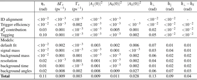
The systematic uncertainties are provided in Table 7. For each variable, the total systematic error is

obtained adding in quadrature the different contributions.

Table 7: Summary of systematic uncertainties assigned to parameters of interest.

φs ∆Γs Γs |A_k(0)|² |A0(0)|² |A_S(0)|² δ_⊥ δ_k δ_⊥−δ_S

(rad) (ps⁻¹) (ps⁻¹) (rad) (rad) (rad)

ID alignment <10⁻² <10⁻³ <10⁻³ <10⁻³ <10⁻³ - <10⁻² <10⁻² - Trigger efficiency <10⁻² <10⁻³ 0.002 <10⁻³ <10⁻³ <10⁻³ <10⁻² <10⁻² <10⁻² B⁰_dcontribution 0.03 0.001 <10⁻³ <10⁻³ 0.005 0.001 0.02 <10⁻² <10⁻² Tagging 0.10 0.001 <10⁻³ <10⁻³ <10⁻³ 0.002 0.05 <10⁻² <10⁻² Models:

default fit <10⁻² 0.002 <10⁻³ 0.003 0.002 0.006 0.07 0.01 0.01 signal mass <10⁻² 0.001 <10⁻³ <10⁻³ 0.001 <10⁻³ 0.03 0.04 0.01 background mass <10⁻² 0.001 0.001 <10⁻³ <10⁻³ 0.002 0.06 0.02 0.02

resolution 0.02 <10⁻³ 0.001 0.001 <10⁻³ 0.002 0.04 0.02 0.01

background time 0.01 0.001 <10⁻³ 0.001 <10⁻³ 0.002 0.01 0.02 0.02

background angles 0.02 0.008 0.002 0.008 0.009 0.027 0.06 0.07 0.03

Total 0.11 0.009 0.003 0.009 0.011 0.028 0.13 0.09 0.04

8 Discussion

The PDF describing the B

⁰_s→

J

/ψ φ

decay is invariant under the following simultaneous transformations:

{φ_s,∆Γ,δ⊥,δ_k} →(π−φs,−∆Γ,π−δ⊥,2π−δ_k)

∆Γs

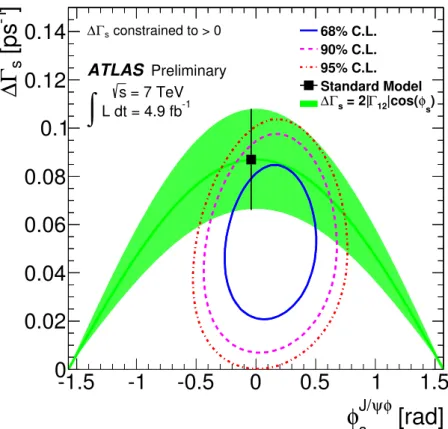
has been determined to be positive [19]. Therefore there is a unique solution. Uncertainties on individual parameters have been studied in details in likelihood scans. Figure 7 shows the 1D likelihood scans for

φs

and

∆Γs

. Figure 8 shows the likelihood contours in

φs

-

∆Γs

plane.

[rad]

φs

-3 -2 -1 0 1 2 3

-2 ln(L)

0 5 10 15 20 25

ATLASPreliminary L dt = 4.9 fb-1

∫

^{s = 7 TeV}

-1]

s [ps Γ

∆

0 0.05 0.1 0.15 0.2

-2 ln(L)

0 10 20 30 40

50 ^ATLASPreliminary L dt = 4.9 fb-1

∫

^{s = 7 TeV}

Figure 7: 1D likelihood scans for

φs

(left) and

∆Γs

(right)

The behaviour of the amplitudes around their fitted values is as expected, however the strong phases are more complicated. Figure 9 shows the 1D likelihood scans for the three measured strong phases.

The behaviour of

δ⊥

appears gaussian and therefore it is reasonable to quote

δ⊥=

3.89

±

0.47(stat)

rad. For

δ⊥−δS

the the likelihood scan shows a minimum close to

π

, however it is insensitive over

[rad]

φ ψ J/

φ

s

-1.5 -1 -0.5 0 0.5 1 1.5

]

-1

[ps

s

Γ ∆

0 0.02 0.04 0.06 0.08 0.1 0.12

0.14

∆Γs constrained to > 0

ATLAS Preliminary = 7 TeV s

L dt = 4.9 fb-1

∫

68% C.L.

90% C.L.

95% C.L.

Standard Model

s)

|cos(φ Γ12

= 2|

Γs

∆

Figure 8: Likelihood contours in

φs

-

∆Γs

plane. The blue and red contours show the 68% and 95%

likelihood contours, respectively (statistical errors only). The green band is the theoretical prediction of mixing- induced CP violation.

[rad]

δ||

2.4 2.6 2.8 3 3.2 3.4 3.6 3.8 4

-2 ln(L)

0 10 20 30 40 50 60 70 80 90 100

ATLASPreliminary L dt = 4.9 fb-1

∫ ^{s = 7 TeV}

[rad]

δ

0 1 2 3 4 5 6

-2 ln(L)

0 2 4 6 8 10 12 14 16 18

ATLASPreliminary L dt = 4.9 fb-1

∫ ^{s = 7 TeV}

[rad]

δS

δ -

0 1 2 3 4 5 6

-2 ln(L)

0 1 2 3 4 5 6 7 8 9 10

ATLASPreliminary L dt = 4.9 fb-1

∫ ^{s = 7 TeV}

Figure 9: 1D likelihood scans for

δ||

(left),

δ⊥

and

δ⊥−δS

(right)