SFB 823
Testing for structural changes in large portfolios
Discussion Paper
Peter N. Posch, Daniel Ullmann,Dominik Wied
Nr. 32/2015
1
Testing for structural changes in large portfolios
Peter N. Posch1, Daniel Ullmann2, Dominik Wied3 First draft: June 2015 This version: August 2015
Abstract
Model free tests for constant parameters often fail to detect structural changes in high dimensions. In practice, this corresponds to a portfolio with many assets and a reasonable long time series. We reduce the dimensionality of the problem by looking a compressed panel of time series obtained by cluster analysis and the principal components of the data.
Using our methodology we are able to extend a test for a constant correlation matrix from a sub portfolio to whole indices and exemplify the procedure with the EuroStoxx index.
Keywords: correlation, structural change, cluster analysis, portfolio management JEL Classification: C12, C55, C58, G11
Acknowledgement. Financial support by the Collaborative Research Center “Statistical Modeling of Nonlinear Dynamic Processes” (SFB 823) of the German Research Foundation (DFG) is gratefully acknowledged.
1 Technical University of Dortmund, Faculty of Business, Economics and Social Science, 44227 Dortmund, Germany, email peter.posch@udo.edu
2 Technical University of Dortmund, Faculty of Business, Economics and Social Science, 44227 Dortmund, Germany, email daniel.ullmann@udo.edu. *Corresponding author
3 Technical University of Dortmund, Faculty of Statistics, 44227 Dortmund, Germany, email wied@statistik.tu- dortmund.de
2 1 Introduction
Portfolio optimization is most often based on the empirical moments of the returns of portfolio constituents, where the diversification effect is based on some measure of pairwise co-movement between constituents, e.g. correlation. Whenever the characteristics of either the individual moments or the correlation changes, the portfolio’s optimality is affected. Thus, it is important to test for the occurrence of changes in these parameters and there exist tests for detecting retrograde structural breaks, (see Andreou & Ghysels (2009);
Aue & Horváth (2013) for an overview). In this paper, we investigate in detail potential changes in correlation. In the last few years, there is a growing interest in the literature for detecting breakpoints in dependence measures, especially for the case that the time of potential breaks need not be known for applying the test. People look, e.g., at the whole copula of different random variables (Bücher et al. 2014), but also at the usual bivariate correlation (Wied et al. 2012). The motivation for such approaches comes from empirical evidence that correlations are in general time-varying (see Longin and Solnik 1995 for a seminal paper on this topic), but it is unclear whether this is true for both conditional and unconditional correlations.
In the following, we consider a nonparametric fluctuation test for a constant correlation matrix proposed by Wied (2015). This test, as many others constructed in similar fashion, needs a high number of time observations relative to the number of assets for sufficient size and power properties. In practice, a typical multi asset portfolio has several hundreds of assets under management, but the joint time series for all assets is considerably smaller.
So how can we test for a structural break of the correlation structure of a portfolio where the number of assets is large and possibly larger than time observations?
Our approach is to reduce the dimensionality and then applying the Wied (2015) test to the reduced problem.
We consider two approaches to reduce the dimension of the problem. First, we employ cluster analysis, second principal component analysis, cf. e.g. Fodor (2002) for a discussion of their use in dimensionality reduction. Cluster analysis has a wide range of applications such as biology (Eisen et al. (1998)), medicine (Haldar et al. (2008)) and finance (Bonanno et al. (2004); Brida & Risso (2010); Mantegna (1999a); (b);
Tumminello et al. (2010)), where it is also applied in portfolio optimization (Onnela et al. (2002), (2003);
Tola et al. (2008)). Yet, as far as we know, we are the first to combine clustering and tests for structural breaks, which might be an interesting contribution to the existing literature on portfolio optimization.
The principal component analysis (PCA) dates back to Pearson (1901) and is “one of the most useful and most popular techniques of multivariate analysis” (Hallin et al. (2014)) with wide applications in finance, cf. Greene (2008) or Alexander (2008). It is suitable for reducing the dimensionality of a problem (Fodor
3
(2002)), since its central idea is the transformation and dimension reduction of the data, while keeping as much variance as possible (Jolliffe (2002)).
The structure of the paper is as follows: In Section 2 we develop the test for structural changes in a large portfolio context. In Section 3 we apply the test to a real-life data set, report the resulting clusters and present the result of our analyses, while the final Section 4 concludes.
2 Methodology
In this section we develop the test approach to detect structural breaks in a large portfolio’s correlation structure. The basis for our analysis is the correlation matrix:
ρ = (ρi,j)
i,j=1,…,n where 𝜌𝑖,𝑗 =𝐸((𝑥𝑖−𝜇𝑖)(𝑥𝑗−𝜇𝑗))
√𝜎𝑗2𝜎𝑖2
, ( 1 )
with 𝜇𝑖 as the first moment and 𝜎𝑖2 as the variance of the corresponding time series. For the estimator ρ̂ we use the empirical average 𝜇̂𝑖 and the empirical variance 𝜎̂𝑖2.
Since the estimated correlation matrix has to be positive definite (Kwan (2010)), we need more observations than assets. Looking at n assets with T observations, a sequence of random vectors Xt= (X1,t, X2,t, … , Xn,t), we calculate the correlation matrix from the first k observations according to equation ( 1 ) and denoted as ρ̂𝑘.
We set the hypotheses as H0: ρt= ρt+τ ∀ t = 1 … T, τ = 1 … T − t vs. H1: ∃t, τ: ρt≠ ρt+τ and define the difference to the correlation matrix from all T observations as
P̂k,T = 𝑣𝑒𝑐ℎ (ρ̂k− ρ̂T), ( 2 ) where the operator 𝑣𝑒𝑐ℎ(𝐴) denotes the half-vectorization:
𝑣𝑒𝑐ℎ(A) = (𝑎𝑖,𝑗)
1≤𝑖<𝑗≤dim (𝐴). ( 3 )
The test statistic is given by Wied (2015) as ÂT≔ max
2≤k≤T k
√T‖Ê−12 P̂k,T‖
1 , ( 4 )
where ‖ ‖1 denotes the L1 norm. The null is rejected if ÂT exceeds the threshold given by the 95% quantile of A with the following definition:
4 A ≔ sup
0≤𝑠≤1‖Bn(n−1)2 (𝑠)‖
1
( 5 )
Here Bk(𝑠) is the vector of 𝑘 independent standard Brownian Bridges.
If the test statistic exceeds this threshold, we define the structural break date 𝑘 as the following time point:
argmax
𝑘
𝑘
√𝑇|P̂k,T|. ( 6 )
For the limiting distribution of the statistic we need a scaling matrix 𝐸̂ , which can be obtained by bootstrapping in the following way:
We define a block length 𝑙 and divide the data into 𝑇 − 𝑙 − 1 overlapping blocks: 𝐵1 = (𝑋1, … , 𝑋𝑙), 𝐵2= (𝑋2, … , 𝑋𝑙+1), …
In each repetition 𝑏 ∈ [1, 𝐵] for some large B, we sample ⌊𝑇
𝑙⌋ times with replacement one of the blocks and merge them all to a time series of dimension 𝑙 ⋅ ⌊𝑇
𝑙⌋ × 𝑛.
For each bootstrapped time series we calculate the covariance matrix. We convert the scaled elements above the diagonal to the vector 𝑣̂𝑏 = √𝑇(𝜌̂𝑏,𝑇𝑖,𝑗)
1≤𝑖<𝑗≤𝑛
We denote the covariance of all these vectors with 𝐸̂ ≔ 𝐶𝑜𝑣(𝑣̂1, … , 𝑣̂𝐵)
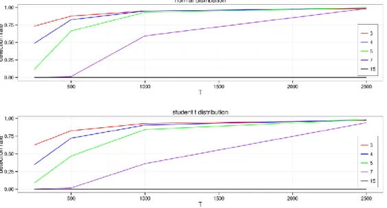
For the original test to provide a good approximation of the limiting distribution the ratio of observations to assets needs to be much larger than one. A portfolio with a large number of assets and insufficient time length of observation thus cannot be analyzed with the present test for structural changes in its correlation matrix. As Figure 1 shows, the detection rate of test decreases nonlinear with increasing number of assets.
We simulated correlated time series from both a normal and a student t distribution with three degrees of freedom. The break in the correlation is placed in the middle of the test. For only 15 assets, we are not able to detect one break, even when using 2500 data points, which corresponds to roughly 10 years of historic prices.
<Insert Figure 1 here>
We will thus discuss two techniques, clustering and principal component analysis, to reduce the dimensionality of the problem and apply the test afterwards. A first approach is to use exogenous clusters such as e.g. industry sectors which, however, imposes an exogenous structure possibly not present in the data. Clustering endogenously based on the present correlation structure instead preserves this information
5
cf. Mantegna (1999b), an approach which is applied widely, e.g. in financial markets by Brida & Risso (2010), in medicine by Eisen et al. (1998)).
The first step is to transform the correlation into a distance metric d fulfilling the following four requirements (7)-(10) where in the application of a clustering algorithm (10) is replaced by the stronger (10a), since an ultra-metric is used.
𝑑(𝑥, 𝑦) ≥ 0 (7)
𝑑(𝑥, 𝑦) = 0 ⇔ 𝑥 = 𝑦 (8)
𝑑(𝑥, 𝑦) = 𝑑(𝑦, 𝑥) (9)
𝑑(𝑥, 𝑧) ≤ 𝑑(𝑥, 𝑦) + 𝑑(𝑦, 𝑧) (10)
𝑑(𝑥, 𝑧) ≤ max {𝑑(𝑥, 𝑦), 𝑑(𝑦, 𝑧)} (10a) Following Anderberg (1973) and Mantegna (1999b) we use
𝑑(𝑥𝑖, 𝑥𝑗) = √2(1 − 𝜌𝑖,𝑗) , (11) which is the Euclidean distance between the standardized data points 𝑥𝑖 and 𝑥𝑗. The metric is bounded in the interval 𝑑 ∈ [0,2] and smaller values correspond to a smaller distance and thus to more similarity. The clustering algorithm itself runs as follows:
1. Find the pair 𝑖, 𝑗 which satisfies 𝑑(𝑥𝑖, 𝑥𝑗) = min
𝑚,𝑛𝑑(𝑥𝑛, 𝑥𝑚) 2. Merge the pair 𝑖 and 𝑗 into a single cluster
3. Calculate the distance to the other clusters 4. Repeat steps 1 and 2 as often as desired
In the calculation of the distance in the third step we choose the following approaches
Complete linkage: the distance to the other clusters is set to the maximum of the two distances of the merging clusters (Anderberg (1973)). The maximal distance corresponds to a minimum in the absolute value of the correlation.
Single linkage: the distance to the other clusters is determined by the minimum of the two sets to be merged (Anderberg (1973); Gower & Ross (1969)). The minimal distance corresponds to a maximum in the absolute value of the correlation.
Average linkage: the distance to the remaining clusters is calculated as the equally weighted average of all merged cluster elements (Anderberg (1973)).
6
Furthermore we apply the ward algorithm, where the criterion for selecting two clusters to merge is such that the variance within them becomes minimal Anderberg (1973); Murtagh & Legendre (2014); Ward Jr (1963). This approach should lead to the most homogeneous clusters, while our three linkage algorithms are based on the correlation with the complete linkage reacting most conservative to correlation, the single linkage most aggressively and the average linkage providing a middle way between these two.
All algorithms result in a hierarchical tree as shown in Figure 3. The tree itself does not make any statement about the clusters. Instead they are formed by cutting the hierarchical tree horizontally at a height such that the desired amount of clusters is formed.
Since all four algorithms result in different clusters for the same chosen height we add the concept of equally sized clusters to choose among the results: If we seek to form 𝑚 clusters out of 𝑛 assets and one of them contains 𝑛 − 𝑚 + 1 assets, we end up with the most unequal cluster size possible. In this extreme case the likelihood for a randomly chosen asset to be in the one large cluster is highest and its cluster weight lowest.
In contrast clusters are uniformly distributed in size the sensitivity of the cluster formation is higher. To gain a homogenously sized clustering we use the (Herfindahl) Hirschman index (Hirschman (1964), (1980)).
In a final step we transform the each cluster into a cluster-portfolio, which is a subportfolio of the initial portfolio of all assets. To determine each cluster-portfolio asset’s weights we can use the initial weights from the overall portfolio, e.g. if decomposing the EuroStoxx 50, an European stock market index containing the 50 largest stocks by market capitalization, we would use the weight each asset has in the EuroStoxx as individual weight in the cluster-portfolio. Secondly we can transfer the methodology used in the original portfolio composition to the cluster-portfolio, e.g. the EuroStoxx weights constituents according to their market capitalization relative to the full index. Applying this to the cluster-portfolio would weight each asset relatively to the cluster-portfolio’s market capitalization. Both methods impose an external structure which is (possibly) relevant for investing but not for the detection of structural changes.
We thus stick to the third option of equally weighting all assets within each cluster-portfolio.
This concludes the clustering approach. We now turn to the use of principal component analysis (PCA) as an alternative technique to reduce the dimensionality. The PCA projects given data 𝑋 in the high dimensional Cartesian coordinate system into another orthonormal coordinate system based on the eigenvalue decomposition of the covariance matrix of the given data.
Let Σ = 𝑉𝑎𝑟(𝑋) ∈ ℝ𝑛×𝑛 denote the empirical covariance matrix. Than there exists a transformation Bronstein et al. (2012) defined as:
7
Σ = 𝑃 Λ 𝑃′ , Λ ∈ ℝ𝑛×𝑛 , 𝑃 ∈ ℝ𝑛×𝑛 (12) where 𝑃 is the matrix formed by the eigenvectors of Σ and Λ as a diagonal matrix with the eigenvalues 𝜆𝑖 on its diagonal.
The matrix of principle components is calculated as 𝑍 = X 𝑃. This is the representation of the given data in the eigenvector coordinate system. For the variance of the “rotated” data we get
𝑉𝑎𝑟(𝑍) = 𝐶𝑜𝑣((X 𝑃)′, X 𝑃) = 𝐶𝑜𝑣(𝑃′X′, X 𝑃) = 𝑃′𝐶𝑜𝑣(X′, X)𝑃 = 𝑃′Σ𝑃 = Λ (13) which is a diagonal matrix and therefore uncorrelated data in the rotated system.
By using only the k largest eigenvalues, we can now reduce the dimensions in the orthonormal base. The obtained data is an approximation of the original data but with only k dimensions in the orthonormal base and 𝑛 dimensions in the Cartesian space, cf. Hair (2010).
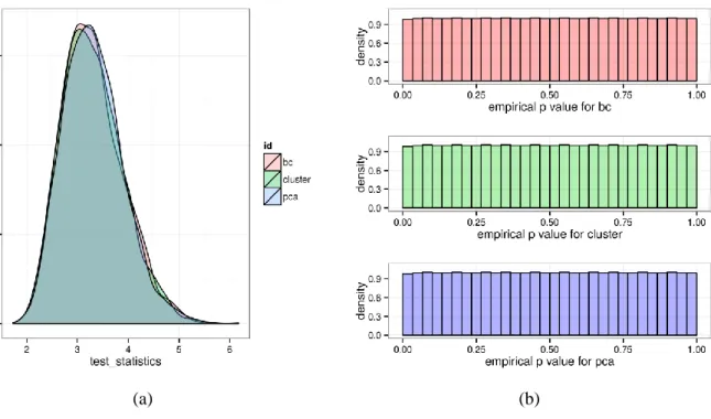
The two methods of clustering and PCA are two approaches to reduce the dimension of the problem at hand resulting in a linear transformation of the given data and forming actually indices or sub-portfolios, which are analyzed in the Euclidean or another “Eigen” space. Due to the nature of the transformation the limiting distribution of the original data is preserved. We verify this preservation by simulating 2500 realizations of 1000 assets with 1500 time points and a fixed random correlation matrix. We randomly choose the eigenvalues in the interval [1, 10] and use the columns of a random orthogonal matrix as the corresponding eigenvectors. Figure 2 shows the histogram of the test statistic on the left hand side and the corresponding empirical p values on the right hand side. As the p values seem to be uniformly distributed, we can conclude, that the limiting distribution does not change.
<Insert Figure 2 here>
8 3 Application to a real-life problem
We now turn to the application of the before mentioned methods. We use the EuroStoxx 50 index which is a widely used index on European stock markets, consisting of the 50 largest, by market capitalization, stocks traded publicly in European countries. We obtain the most current index composition4 and individual stock prices for these constitutions from July 2005 – March 2015. Based on this sample we form four portfolios:
(i) The portfolio of Wied (2015) which consists of four stocks from the EuroStoxx index: BASF, Sanofi, Siemens for the time span Jan 2007 - June 2012.
(ii) An extension of the portfolio in (i) with 21 other, randomly chosen stocks from the remaining index constitutions during the same period. This results in a portfolio of 25 stocks and thus half of the EuroStoxx50 index.
(iii) The full EuroStoxx 50 over the same time period as in (i) and (ii).
(iv) The full EuroStoxx 50 index with all 50 stocks for the full time period 2005-15.
To mimic the setting of Wied (2015) we cluster the portfolios (ii), (iii) and (iv) into four cluster-portfolios as described in the previous section and shown in Figure 3. The most homogenous clusters concerning the size are obtained with the ward algorithm.
<Insert Figure 3 here>
To illustrate the difference to the exogenous sector-clustering provided by the index company we color each constituent with the corresponding sector color. The clusters do not become totally homogenous, concerning the industry sector, when increasing the number of assets monitored (Figure 3 (b)). As an example, when monitoring all 50 assets, Deutsche Telekom and Telefonica are not placed in one cluster (see Table 3). This means, the inevitable error generated by the clustering would be bigger using the exogenous industry sectors, since companies from two different sectors may perform more similar than two in the same sector.
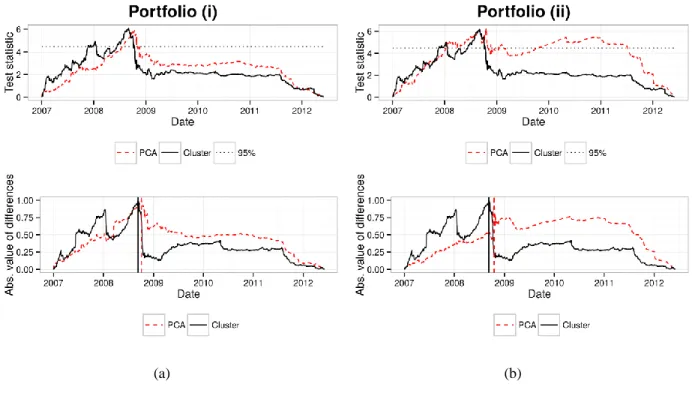
In the discussion of the results we use portfolio (i) as base case and show the result of the structural change test in Figure 4 (a). In the upper part, we see the actual test statistic for the clusters in black and the principal components in the red, dotted line. The horizontal line denotes the critical value 4.47, which corresponds to a confidence level of 95%. A structural change is detected if the test statistic exceeds the critical value,
4 We are aware that this does not mimic constituent changes and would result in a selection bias with respect of modelling the EuroStoxx50. As our goal, however, is to demonstrate the methodology developed and not to provide a model for this particular index, we proceed without this additional restriction.
9
while the actual break date is given at the maximum of the absolute difference between the corresponding matrices. This difference is plotted in the lower graph scaled to one. Again, the black line shows the difference for the clusters and the dotted red line the differences for the principal components. We detect structural changes at the 443th data point which is 11th September 2008 in calendar date and the 460th data point, corresponding to 6th October 2008, in line with Wied (2015). Turning to portfolio (ii) we randomly add 21 stocks during the same period as an intermediate stage, see Table 2 for the portfolio composition.
The four resulting clusters are shown in Figure 3 (a).
<Insert Figure 4 here>
The result of the structural change test is shown in Figure 4 (b) with the previously described legend. The indicated break dates, as shown in the lower part of Figure 4 (b), refer to the 11th September 2008 (443rd data point) and to the 21st October 2008 (471st data point). In the PCA case, we are able to preserve 73.6%
of the overall variation. While it’s break dates lag slightly by 15 days, the clusters’ dates remain unchanged to the base case.
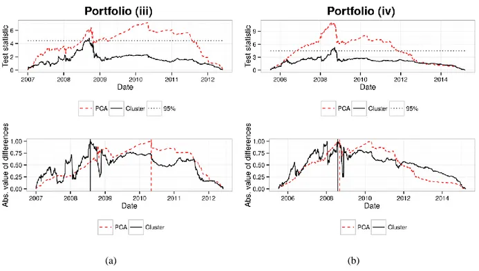
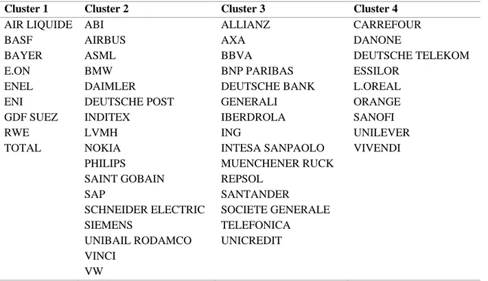
Turning to our full portfolio (iii) and (iv). The formation of the clusters is shown in Figure 3 (b) and Table 3 shows the cluster’s composition. The difference between these two is the monitored time span. In (iii) we use the same period than before and in (iv) we use all given information.
<Insert Figure 5 here>
When we look at the principal components, we are able to capture 65.8% of the overall variation in the data with the first four eigenvalues in both portfolios. The resulting test statistics of the structural break test are shown in Figure 5 (a) and (b). We see significant structural break both in the PCA and the clusters. The corresponding break dates are the 30th July 2008 (413th data point) and 2nd May 2010 (870th data point) in the case of portfolio (iii). We see a lag of nearly 2 years compared to portfolio (ii). It is shifted towards the one in portfolio (ii) when the time interval is increased to the whole data set in portfolio (iv). Here the corresponding break dates are the 29th July 2008 (800th data point) and the 3rd September 2008 (826th data point). Compared to the results of portfolio (ii) we see that we now obtain leads which can be due the full information set used. With this sample we illustrated the use of a test for changes in the correlation matrix on a large portfolio where the number of assets does not allow a direct application of the test. Instead we propose two methods, clustering and PCA, to reduce the dimension prior to applying the test. While the results show the usefulness of these approaches, we now turn to the discussion of its robustness.
<Insert Figure 6 here>
10
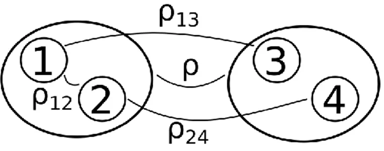
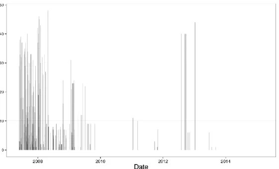
One question concerning the cluster approach is the stability of the clusters over time. Consider Figure 6 where we illustrate four assets (circles) of which two clusters (ellipses) are formed. In the above described clustering approach, we only use the correlation between the clusters 𝜌 and not (explicitly) the correlation within the clusters 𝜌12 and between assets in different clusters 𝜌13 and 𝜌24. Thus we are able to detect a structural break only in the correlations between clusters in the first place. To see if clusters remain constant over time we calculate the cluster members for each time point from [𝑡0+ 100, 𝑇], choosing a lag of 100 data points to get a stable first estimate. The results for our portfolio (iv) is shown in Figure 7. For each time point we compare the cluster members with the previous time point. Summing up the numbers of jumps, we yield the stated figure. We can conclude that cluster changes occur frequently especially at the beginning of the time interval which corresponds to the stability of the correlation matrix’ estimation.
<Insert Figure 7 here>
Thus the question remains if changes within a given cluster (e.g. 𝜌12) are detectable by the test. We simulate four normal distributed variables correlated with a given correlation matrix. We use time series with lengths {500, 1000, 1500, 2000} data points. To simulate a larger cluster, in which only one asset changes the within correlation, we set the weights randomly in the interval (i) [0.1, 0.5], (ii) [0.01, 0.05] and (iii) [0.5, 0.01]. So we can compare the behavior for small (i) and large (ii) clusters. Case (iii) serves as an overall assessment.
As the starting point we chose the matrix
𝜌0= ( 1
0.7717 1
0.2597 0.1328 1
−0.0589 0.1665 0.8523 1 )
which is positive semi definite and has a high correlation between assets 1 and 2 and assets 3 and four.
This matrix results in the desired clusters. We now distinguish the following cases:
a) We change only 𝜌12: This corresponds to fluctuations within a cluster that are not so large that the asset would leave the cluster. To do this, we set this value to a random number in the interval [0.7 , 1.0].
b) We decrease 𝜌12 and increase 𝜌23, 𝜌24: This corresponds to a change of the cluster members in a way, that assets 2, 3 and 4 build a cluster. In order to simulate this, we set 𝜌12∈ [−0.2 , 0.2], 𝜌32∈ [0.6 , 1.0], 𝜌42 ∈ [0.6 , 1.0].
11
c) We change the correlations of assets 2 and 3: This corresponds to a situation where a new clustering would result in a cluster of asset 1 and 3 and a cluster of asset 2 and 4. Thus we set 𝜌12∈ [−0.2 , 0.2], 𝜌13 ∈ [0.6 , 1.0], 𝜌24∈ [0.6 , 1.0], 𝜌34∈ [−0.2 ,0.2].
In all cases we draw from the given interval until a positive semi definite matrix with the desired entries is obtained which is then used to change the time series’ correlation at the middle of the simulated time span. Table 1 reports the detection rate of test, where “base case” refers to the situation where we have just two equally weighted assets in each of the two clusters
In all cases, we see the decreasing detection rate with an increasing confidence interval. Starting with case a) we see a rate of about 75% at the 90% quantile, it drops to about 15% for the 99% quantile. Compared to the case b) and c) these are rather poor detection rates, since the fluctuation in the true correlation structure is rather small. In the two latter cases, the detection rates are comparable high. Since the structure is changed more drastically, these changes can be detected in the overall cluster time series. Concluding we find that the structural break test is not only able to detect breaks between clusters, but it may also be able to detect larger fluctuations within (unchanged) clusters. But this does not mean that finding no breaks between clusters means that there are no breaks within clusters.
A second important issue is the robustness with changing weights of the assets in the cluster-portfolios, as illustrated by the following case. Assuming normalized variances, we can calculate the correlation between the above given clusters as
𝐶𝑜𝑣( [1,2], [3,4]) = 𝑤1𝑤3𝜌13+ 𝑤1𝑤4𝜌14+ 𝑤2𝑤3𝜌23+ 𝑤2𝑤4𝜌24 (14) d𝐶𝑜𝑣( [1,2], [3,4]) = 𝑤1𝑤3d𝜌13+ 𝑤1𝑤4d𝜌14+ 𝑤2𝑤3d𝜌23+ 𝑤2𝑤4d𝜌24 (15)
When each asset is equally weighed, a change d𝜌13= −d𝜌24 leads to a change in the correlation of d𝐶𝑜𝑣( [1,2], [3,4]) = 0 (ceteris paribus). Thus, such a change in the correlation between one pair of assets which is offset by an opposite change of another pair cannot be detected as there is no change in the correlation between the clusters.
While this constructed example is unlikely to occur in practice, a change in the weights from an equal distribution has a direct influence on the test’s power: the sensitivity increases in the direction in which the weight is increased.
Another concern comes with the application of the PCA. As the dimensions increases, i.e. the number of assets of the initial portfolio relative to the time span available raises, we have to neglect relatively more
12
dimensions in the basis of the eigenvalues. We are then left only with the high volatile dimensions and a structural break detected therein can be regarded as a very likely and thus most obvious break.
In this light we like to quantify the error made in neglecting small volatile dimensions when applying the PCA. Since variation in the small eigenvalues correspond to noise in the estimation of the true correlation matrix, cf. Laloux et al. (1999), (2000); Plerou et al. (2002), the exclusive use of the data from the eigenvalues that are larger than a threshold given by the random matrix theory is suggested. Generally it is not true that a reduction in the percentage of variation represented by the first k eigenvalues likewise reduces the likelihood of detecting a structural break in the data. Improving the accuracy of the estimated correlation may even be the case, since noise has been neglected. Concluding, we only have to worry about the information associated with eigenvalues, which are smaller than the fourth largest eigenvalue and larger then this threshold eigenvalue.
4 Conclusion
Monitoring the correlation matrix of a portfolio is a daily task in financial portfolio management and modern portfolio optimization heavily relies on the matrix in calculating the portfolio weights. Likewise triggers the occurrence of changes in this correlation structure, a structural break, a portfolio adjustment.
While test for structural breaks are readily available and discussed in the literature, they can only deal with a low number of assets, e.g. Wied (2015) with only four assets. In practice, however, we most commonly have a situation in which the number of assets by far exceeds the available time series. Thus so far no test on structural changes in the correlation structure of typical portfolios was possible.
We discuss this problem and offer two approaches to deal with this problem resulting in a working algorithm for such high dimensional, or complex, portfolios. Our approaches, clustering and principal component analysis, reduce the dimension in a first stage. In a second stage a test on structural changes is then applied to the reduced problem.
With these approaches, we reproduce previous results from the literature as first consistency check. We then turn to a larger setting using a common portfolio on stocks in the Eurozone and demonstrate the proposed algorithms’ power.
Furthermore we discuss extensively the robustness of this algorithm and use excessive Monte Carlo simulation to show that by forming subportfolios we are not restricted to detecting structural breaks between clusters.
13
Figure 1. Detection rate of the test for constant correlation
The figure shows the power of the test for constant correlation in a simulated setup. We simulated time series with lengths 250, 500, 1000, 2500 data points and placed the break in the correlation in the middle of each series. The upper plot shows the detection rate based on critical values from a normal distribution while the lower uses a student t distribution with 3 degrees of freedom.
14
Figure 2. Test statistics and empirical p values for the cluster and PCA approach
On the left hand side, the figure shows the estimated density of the test statistic for both the cluster and the PCA approach. The original test statistic of Wied (2015) with 4 assets is denoted with bc. The right hand side shows the corresponding p values for all three cases.
(a) (b)
15 Figure 3. Hierarchical trees and cluster sizes
In the upper part, the figure (a) shows the hierarchical trees for the portfolio (ii) and figure (b) for the portfolio (iii) and (iv). The trees are formed by the Ward algorithm. They are cut horizontally to form the four clusters. On the lower end of the trees we denoted the several companies and colored them according to their supersector. In the lower part of the figure, the number of cluster constituents is shown.
(a) (b)
16
Figure 4. Test statistic and break detection for portfolio (i) and (ii)
The figures show the resulting test statistics in the upper half and the scaled break detection in the lower half. The black solid lines correspond to the cluster approach and the red dashed lines to the PCA approach.
The 95% confidence level is denoted by the black dotted line and the break dates are highlighted by the corresponding vertical lines.
(a) (b)
17
Figure 5. Test statistic and break detection for portfolio (iii) and (iv)
The figures show the resulting test statistics in the upper half and the scaled break detection in the lower half with the same definitions like in Figure 4. The black solid lines correspond to the cluster approach and the red dashed lines to the PCA approach. The 95% confidence level is denoted by the black dotted line and the break dates are highlighted by the corresponding vertical lines.
(a) (b)
18
Figure 6. Notation for correlations within and between clusters
Shown are four assets (circles), where two assets are included in a cluster (ellipse). The correlation between clusters is denoted as 𝝆 and the correlation between assets 𝒊, 𝒋 as 𝝆𝒊,𝒋.
19
Figure 7. Number of jumps between two consecutive periods
We plot the number of jumps of cluster members compared to the ones in the previous period on the y-axis.
The analysis is done with portfolio (iv).
20 Table 1. Detection rate of the cluster approach
We generated normal distributed time series of length 500, 1000, 1500 and 2000 data points. Thereof we form four clusters, where the weights are dependent on the cases. Base case has four assets, (i) 10-20 assets, (ii) 20-100 assets and (iii) 10-100 assets. The correlation structure was changed in the middle of the time series, depending on the scenario (a) with within fluctuation, (b) with an asset outflow or (c) with a switch of assets. For details, see Section 3. We report the detection rate of the resulting break in percent for all 12 possible combinations.
(a) (b) (c)
Confidence Time length Time length Time length
in % 500 1000 1500 2000 500 1000 1500 2000 500 1000 1500 2000
Base 90 76 76 73 78 100 100 100 100 100 100 100 100
Case 95 49 48 42 50 100 100 100 100 100 100 100 100
99 13 15 10 13 100 100 100 100 100 100 100 100
(i) 90 76 75 73 77 96 98 99 100 99 100 100 100
95 49 46 44 48 90 95 97 98 97 99 100 100
99 15 12 11 12 75 85 90 94 91 97 99 99
(ii) 90 77 78 75 78 77 79 77 78 78 78 74 79
95 48 49 45 49 50 51 49 51 50 50 47 50
99 15 13 12 14 16 15 15 18 17 15 14 15
(iii) 90 74 73 71 73 92 94 95 97 96 98 98 99
95 45 44 41 44 82 87 89 91 90 95 96 98
99 13 11 10 12 64 74 78 81 80 89 91 94
21
Table 2. Constituents and clusters of the 50% EuroStoxx 50 portfolio
The table shows the constituents used in the portfolio (ii) in section 3. It consists of the four assets tested in Wied (2015) to which 21 randomly chosen assets from the EuroStoxx 50 index are drawn, resulting in 25 assets which corresponds to 50% of the full index. The columns of the table show the results of the clustering.
Cluster 1 Cluster 2 Cluster 3 Cluster 4
ABI INTESA SANPAOLA INDITEX TELEFONICA
AIR LIQUIDE GDF SUEZ ENEL DEUTSCHE TELEKOM
BASF EON IBERDROLA
BBVA
BNP PARIBAS CARREFOUR ENI
SAINT GOBAIN SANOFI
SAP
SCHNEIDER ELECTRIC SIEMENS
SOCIETE GENERALE TOTAL
UNIBAIL RODAMCO UNICREDIT
VW
22
Table 3. Constituents and clusters of the EuroStoxx 50 index
The table shows the constituents used in the portfolio (iii) and (iv) in section 3. They consist of all index members. The columns of the table show the results of the clustering.
Cluster 1 Cluster 2 Cluster 3 Cluster 4
AIR LIQUIDE ABI ALLIANZ CARREFOUR
BASF AIRBUS AXA DANONE
BAYER ASML BBVA DEUTSCHE TELEKOM
E.ON BMW BNP PARIBAS ESSILOR
ENEL DAIMLER DEUTSCHE BANK L.OREAL
ENI DEUTSCHE POST GENERALI ORANGE
GDF SUEZ INDITEX IBERDROLA SANOFI
RWE LVMH ING UNILEVER
TOTAL NOKIA INTESA SANPAOLO VIVENDI
PHILIPS MUENCHENER RUCK
SAINT GOBAIN REPSOL
SAP SANTANDER
SCHNEIDER ELECTRIC SOCIETE GENERALE
SIEMENS TELEFONICA
UNIBAIL RODAMCO UNICREDIT
VINCI VW
23 References
Alexander, C. (2008): Market Risk Analysis: Practical Financial Econometrics, Volume 2.
Anderberg, M.R. (1973): Cluster analysis for applications. DTIC Document
Andreou, E. & E. Ghysels (2009): Structural breaks in financial time series. In: Handbook of financial time series. Springer, pp. 839–870.
Aue, A. & L. Horváth (2013): Structural breaks in time series. Journal of Time Series Analysis (34)1: 1–
16.
Bonanno, G., G. Caldarelli, et al. (2004): Networks of equities in financial markets. The European Physical Journal B-Condensed Matter and Complex Systems (38)2: 363–371.
Brida, J.G. & W.A. Risso (2010): Hierarchical structure of the German stock market. Expert Systems with Applications (37)5: 3846–3852.
Bronstein, I.N., J. Hromkovic, et al. (2012): 1 Taschenbuch der Mathematik. Springer-Verlag.
Bücher, A., Kojadinovic, I, et al. (2014): Detecting Changes in Cross-Sectional Dependence in Multivariate Time Series. Journal of Multivariate Analysis 132, 111-128.
Eisen, M.B., P.T. Spellman, et al. (1998): Cluster analysis and display of genome-wide expression patterns. Proceedings of the National Academy of Sciences (95)25: 14863–14868.
Fodor, I.K. (2002): A survey of dimension reduction techniques.
Gower, J.C. & G. Ross (1969): Minimum spanning trees and single linkage cluster analysis. Applied statistics: 54–64.
Greene, W.H. (2008): Econometric analysis. Granite Hill Publishers.
Hair, J.F. (2010): Multivariate data analysis.
Haldar, P., I.D. Pavord, et al. (2008): Cluster analysis and clinical asthma phenotypes. American journal of respiratory and critical care medicine (178)3: 218–224.
Hallin, M., D. Paindaveine, et al. (2014): Efficient R-estimation of principal and common principal components. Journal of the American Statistical Association (109)507: 1071–1083.
Hirschman, A.O. (1964): The paternity of an index. The American Economic Review: 761–762.
Hirschman, A.O. (1980): 1 National power and the structure of foreign trade. Univ of California Press.
Jolliffe, I. (2002): Principal component analysis. Wiley Online Library.
Kwan, C.C. (2010): The Requirement of a Positive Definite Covariance Matrix of Security Returns for Mean-Variance Portfolio Analysis: A Pedagogic Illustration. Spreadsheets in Education (eJSiE) (4)1: 4.
24
Laloux, L., P. Cizeau, et al. (1999): Noise dressing of financial correlation matrices. Physical review letters (83)7: 1467.
Laloux, L., P. Cizeau, et al. (2000): Random matrix theory and financial correlations. International Journal of Theoretical and Applied Finance (3)03: 391–397.
Longin, F., Solnik, B. (1995): Is the correlation in international equity returns constant: 1960-1990?
Journal of International Money and Finance 14: 3-26.
Mantegna, R. (1999):(a): Information and hierarchical structure in financial markets. Computer physics communications (121): 153–156.
Mantegna, R.N. (1999):(b): Hierarchical structure in financial markets. The European Physical Journal B-Condensed Matter and Complex Systems (11)1: 193–197.
Murtagh, F. & P. Legendre (2014): Ward’s Hierarchical Agglomerative Clustering Method: Which Algorithms Implement Ward’s Criterion? Journal of Classification (31)3: 274–295.
Onnela, J.-P., A. Chakraborti, et al. (2002): Dynamic asset trees and portfolio analysis. The European Physical Journal B-Condensed Matter and Complex Systems (30)3: 285–288.
Onnela, J.-P., A. Chakraborti, et al. (2003): Dynamics of market correlations: Taxonomy and portfolio analysis. Physical Review E (68)5: 056110.
Pearson, K. (1901): LIII. On lines and planes of closest fit to systems of points in space. The London, Edinburgh, and Dublin Philosophical Magazine and Journal of Science (2)11: 559–572.
Plerou, V., P. Gopikrishnan, et al. (2002): Random matrix approach to cross correlations in financial data.
Physical Review E (65)6: 066126.
Tola, V., F. Lillo, et al. (2008): Cluster analysis for portfolio optimization. Journal of Economic Dynamics and Control (32)1: 235–258.
Tumminello, M., F. Lillo, et al. (2010): Correlation, hierarchies, and networks in financial markets.
Journal of Economic Behavior & Organization (75)1: 40–58.
Ward Jr, J.H. (1963): Hierarchical grouping to optimize an objective function. Journal of the American statistical association (58)301: 236–244.
Wied, D. (2015): A nonparametric test for a constant correlation matrix. Econometric Reviews, forthcoming.
Wied, D., W. Krämer, et al. (2012): Testing for a change in correlation at an unknown point in time using an extended functional delta method. Econometric Theory (28)03: 570–589.