Validating multiple structural change models – A case study
Achim Zeileis
aChristian Kleiber
ba Institut f¨ur Statistik & Mathematik, Wirtschaftsuniversit¨at Wien, Austria
bInstitut f¨ur Wirtschafts- und Sozialstatistik, Universit¨at Dortmund, Germany
SUMMARY
In a recent article, Bai and Perron (2003, Journal of Applied Econometrics) present a comprehensive discussion of computational aspects of multiple structural change models along with several empirical examples. Here, we report on the results of a replication study using theRstatistical software package. We are able to verify most of their findings; however, some confidence intervals associated with breakpoints cannot be reproduced. These confidence intervals require computation of the quantiles of a nonstandard distribution, the distribution of the argmax functional of a certain stochastic process. Interestingly, the difficulties appear to be due to numerical problems inGAUSS, the software package used by Bai and Perron.
Keywords: structural change, breakpoints, econometric software, numerical accuracy, repro- ducibility,R,GAUSS.
JEL classification: C220, C870.
1. INTRODUCTION
Time series with multiple structural changes have recently attracted considerable attention in theoretical and applied econometric literature. Bai (1997) and Bai and Perron (1998) present asymptotic theory for inference on multiple breakpoints, in a companion paper (Bai and Perron, 2003) they provide a comprehensive and detailed discussion of computational aspects as well as several empirical examples.
The present paper aims at replicating the results from Bai and Perron (2003) using theRstatistical software package (RDevelopment Core Team, 2004, seehttp://www.R-project.org/), the GNU implementation of the S language (Chambers and Hastie, 1992), which recently finds increasing attention among econometricians (Cribari-Neto and Zarkos, 1999, Racine and Hyndman, 2002).
Specifically, we employ the R package strucchange (Zeileis, Leisch, Hornik and Kleiber, 2002), which implements a large collection of methods for the analysis of structural change, including fluctuation tests (Kuan and Hornik, 1995),Ftests (Andrews, 1993, Andrews and Ploberger, 1994) as well as methods for the dating and monitoring of structural breaks. Both theRsystem and the strucchangepackage are freely available at no cost under the terms of the GNU General Public Licence (GPL) from the ComprehensiveRArchive Network (CRAN) athttp://CRAN.R-project.
org/. Hence, no access to proprietary software is required to reproduce our results which were obtained usingR1.8.1 and strucchange1.2–2. The results utilizing a kernel HAC estimator also depend on theRpackagessandwich 0.1–2 andzoo0.1–3.
We are able to reproduce most of the results of Bai and Perron, notably estimates of breakpoints and model parameters corresponding to the resulting segmentation. However, for one of the examples, the US ex-post real interest rate, there are marked differences in the confidence intervals associated with the breakpoints. Interestingly, these appear to be due to numerical problems in GAUSS, the software package used by Bai and Perron.
2. REPLICATION
Bai and Perron conducted their analyses using theGAUSSpackage. Their code, which implements a wide array of methods for analyzing multiple structural change models, is available from the JAE data archive in the file brcode.src. Vinod (2000) expresses some doubts on the future of GAUSS in“a world increasingly sympathetic to object oriented languages.”R, on the other hand, offers several notions of object orientation which are specifically designed for programming with data. In particular, theS language has always been advocating a programming style employing integrated and possibly rather complex objects that are able to reflect the conceptual properties of the underlying methods instead of merely returning vectors, matrices and printed output. We therefore present some details regarding the strucchangepackage in order to highlight similari- ties and differences. In particular, the sequence of commands shown with an R prompt (R>) in Section 2.1 are sufficient to reproduce the results for the real interest data.
The model considered is the multiple linear regression model withmbreaks (or, equivalently,m+1 regimes)
yt=x>tβj+ut, t=Tj−1+ 1, . . . , Tj, j= 1, . . . , m+ 1, (1) where T0 = 0 and Tm+1 = T by convention (T is the sample size). Bai and Perron consider a slightly more general setup allowing for partial structural changes, in which only some of the regression coefficients are subject to shifts. The current version ofstrucchangedoes not support partial structural change models. However, this additional feature is not required for two of the three Bai and Perron examples; for the third, estimates of the breakpoints – the parameters of main interest – remain unaffected.
The goal of the analysis is to determine the number and location of the breakpoints Tj, j = 1, . . . , m. As shown by Bai and Perron, under squared-error loss these may be efficiently computed in O(T2) operations using a dynamic programming algorithm for any fixed number of breaksm.
In practice, a search over m is conducted, for m ≤ m∗, where m∗ is fixed by the researcher.
More importantly, a further parameter is at the researcher’s disposal, the minimum fraction of observations allocated to any one segment,, or equivalently, the minimum number of observations per segment, h. This may be considered a bandwidth or trimming parameter; as shown below, results are sometimes quite sensitive to the choice ofh.
2.1 US ex-post real interest rate
We begin with an analysis of the US ex-post real interest rate. Bai and Perron discuss this example in considerable detail, and a filebreak.prg containing the relevant calls to the functions implemented in brcode.src is available from the JAE data archive. This greatly facilitates our task. The data are defined as the three-month treasury bill rate deflated by the CPI inflation rate.
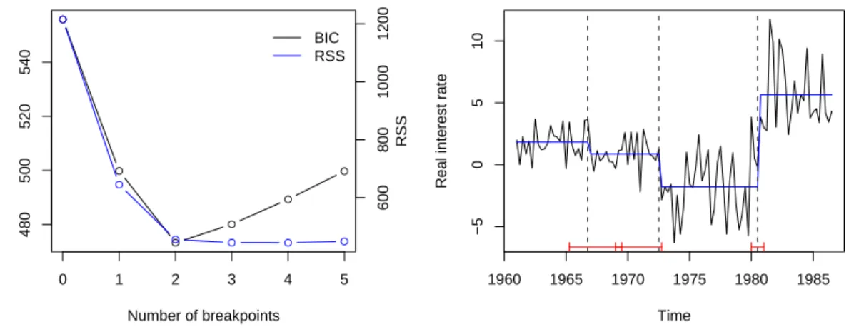
The resulting time series of quarterly data pertaining to the period 1961(3)–1986(3) is depicted in Figure 1.
Here, the series is modelled by only a constant as regressor, the breakpoints are estimated with the strucchangefunctionbreakpointsusing the desired minimal segment sizeh, which may either be specified as a fraction of the sample or as an integer. For these data, a bandwidth parameter of = 0.15 corresponds to the minimal segment size ofh= 15 observations; this amounts to allowing for up tom∗ = 5 breaks. The time series is also available instrucchange, and package and data can be made available by
R> library(strucchange) R> data(RealInt)
In theSlanguage regression relationships are typically specified by a formula notation similar to that of Wilkinson and Rogers (1973): the modelRealInt ~ 1 specifies a linear model in which the dependent variableRealIntis modelled by (~) just an intercept (1):
R> bp.ri <- breakpoints(RealInt ~ 1, h = 15)
The results of the function call tobreakpointsare assigned to an objectbp.rithat comprises a triangular matrix containing the residual sums of squares (RSS) as described by Bai and Perron as well as functions for computing up to m∗ optimal breakpoints from this. The computation of this triangular matrix is the most time-consuming step, all further steps—the extraction of breakpoints, corresponding information criteria, coefficient estimates and confidence intervals—
are left to methods that operate on this objectbp.ri. A summary for all models withm= 1, . . . ,5 breaks along with the corresponding values of the BIC can easily be obtained and visualized by R> summary(bp.ri)
R> plot(bp.ri)
yielding a plot of the RSS and BIC similar to the left panel of Figure 1. Confirming Bai and Perron, information criteria such as the BIC select two breaks. However, on the grounds of sequential tests and also because of the well-known fact that information criteria are often downward-biased, Bai and Perron argue in favor of the presence of an additional break and proceed with a three-break model. Since we are mainly interested in replicating their results, we also consider this three-break model below. Alternatives are briefly discussed at the end of this section.
The regression coefficients and corresponding variances in the three-break model can be extracted via
R> coef(bp.ri, breaks = 3)
R> vcov(bp.ri, breaks = 3, vcov = kernHAC)
These coefficient estimates (with standard errors in parentheses) are given in Table I. The standard errors are estimated utilizing a kernel HAC estimator with a quadratic spectral kernel, prewhiten- ing using a VAR(1) model and an AR(1) approximation for the automatic bandwidth selection, as implemented in thekernHACfunction of theRpackagesandwich. The HAC estimator may be passed to thevcov method as shown above.
Confidence intervals for the breakpoints can be computed from the fitted bp.ri object for any number of breaks (smaller than the maximal number of breaks admissible) using the confint method from strucchange. A function for estimating the covariance matrix, herekernHAC, may again be supplied.
●
●
●
●
●
●
Number of breakpoints
BIC 480500520540
●
●
● ● ● ●
BIC RSS
60080010001200 RSS
0 1 2 3 4 5
Time
Real interest rate
1960 1965 1970 1975 1980 1985
−50510
Figure 1: USex post real interest rate; RSS and BIC for models with up to five breaks (left) and fitted model with three breaks (right).
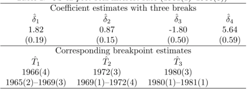
Table I: USex post real interest rate (1961(1)–1986(3)) Coefficient estimates with three breaks
δˆ1 ˆδ2 δˆ3 ˆδ4
1.82 0.87 -1.80 5.64
(0.19) (0.15) (0.50) (0.59)
Corresponding breakpoint estimates
Tˆ1 Tˆ2 Tˆ3
1966(4) 1972(3) 1980(3)
1965(2)–1969(3) 1969(1)–1972(4) 1980(1)–1981(1)
R> confint(bp.ri, breaks = 3, vcov = kernHAC)
This returns the breakpoints and corresponding confidence intervals (at the default 95% level) coded by the observation numbers and by the dates on the underlying time scale. The latter are given in Table I. The fitted model along with the confidence intervals is depicted in Figure 1.
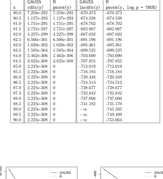
The estimated breakpoints, 1966(4), 1972(3) and 1980(3), as well as the regression coefficients agree with those obtained by Bai and Perron, there are very minor differences regarding the estimated standard errors. Overall, this part of the replication must be considered a success. However, there are considerable differences in the confidence intervals corresponding to the break dates, which cannot be explained by rounding errors in different computing environments. Specifically, the second confidence interval obtained by strucchange (1969(1)–1972(4)) extends much further to the left than the one reported by Bai and Perron (1970(3)–1972(4)). With some effort, we were able to track down the source of the problem, a so-called underflow for which there does not appear to be an easy workaround inGAUSS.
The confidence intervals are derived from the distribution of the argmax functional of a process composed of two independent Brownian motions with different linear drifts and scales; see Bai (1997) for further details on this nonstandard distribution. This cumulative distribution func- tion (CDF) depends on three parameters which, in our application, are associated with ratios of quadratic forms in the magnitude of the shifts and weighting matrices defined as segment-wise covariance matrices.
In the case at hand, the CDF contains terms of the type exp(ax)·Φ(−b√
x), where Φ denotes the CDF of the standard normal distribution, a and b are functions of the residual standard errors pertaining to adjacent segments. For the confidence interval corresponding to the second breakpoint,ais approximately equal to 8.314 whilebis approximately equal to 4.08, and the term must be evaluated forx∈[−10,300] (approximately). Numerically, forxin the vicinity of 300, the term exp(ax)·Φ(−b√
x) is the product of a rather large, exp(ax), and a rather small, Φ(−b√ x), number and it depends on the implementation as well as the routines used by the software package what the latter returns. We looked into this problem utilizing GAUSS v3.2.38, a good proxy for GAUSS v3.2.32, the version used by Bai and Perron.1 Using their program brcode.src, GAUSS v3.2.38 returns values of the CDF up to approximately 0.95 (in fact, only values up to 0.9 are reliable—for larger values the computations cannot yield correct results on a PC as we shall see below), proceeds with some values in excess of 1 (!), and returns infinitely large function values thereafter. This results in a spurious kink in the CDF and in a bisection search (employed for computing the required quantile) stopping near this kink, yielding a 97.5% quantile in the vicinity of 86 and implying that the confidence interval reported by Bai and Perron is not valid. Our R packagestrucchangedoes not produce this spurious kink and returns a 97.5% quantile of 186.45.
What is going on here? At first, this looks like a small programming error that is easy to correct:
coding exp(ax)·Φ(−b√
x) term by term is not a numerically efficient way to handle this quantity.
For largex, Φ(−4.08√
x) is tiny; in fact, forx≥85 it is smaller than the smallest positive number
1We thank Pierre Perron for providing this information.
representable on a PC with 32-bit arithmetic. Columns 2 and 3 of Table II show howGAUSSand R deal with this underflow: Rrounds the probability to the nearest number it can represent—
as computers have to do for any real number—which in this case is 0. GAUSS, on the other hand, argues (as documented on the manual page forcdfn) that the CDF of the standard normal distribution function is always greater than 0 and returns 2.225·10−308, the smallest positive number it can work with. Evidently, neither approximation of the true probability is satisfactory in this situation and the term exp(ax)·Φ(−b√
x) must not be computed via Φ(x) for largex.
A natural solution would be to code the offending term in the form exp(ax+log(Φ(−b√
x))) because 1. the computation of sums is numerically more stable than of products and 2. many software packages for statistics and econometrics (includingGAUSSandR) provide a separate function for computing normal log-probabilities log(Φ(·)) directly. This is used in the implementation of the CDF instrucchangewhich allows us to compute the required 97.5% quantile. (Of course, we do not know what the true quantile is, since there is no benchmark for this nonstandard distribution.
All we can say is that we have no reason to doubt thatRreturns a reasonable approximation to the truth.) However, inGAUSSthe problem turns out to be more serious. While the spurious kink in the CDF disappears, GAUSS for Windows v3.2.38 is unable to go beyond the 90.7% quantile (it returns missing values therafter). Clearly, for two-sided confidence intervals corresponding to conventional confidence levels, at least the 95% and preferably also the 97.5% and 99.5%
quantiles are required. Columns 4 and 5 of Table II and Figure 2 (right panel) exhibit whatGAUSS and Rreturn for log(Φ(−4.08√
x)),x ∈[80,90], utilizing the GAUSS functionlncdfn and its R counterpart pnorm with option log.p = TRUE. Evidently, lncdfn does not improve much upon cdfn: despite the log-probabilities having numerically non-critical values around -750, lncdfn returns−∞forx≥89. In contrast,R returns finite values for much larger arguments. Lacking access to the internals of GAUSS, we can only speculate that either an inaccurate expansion for log(Φ) or a coding error is responsible for these results. A look at the documentation and the code of Rreveals thatpnormutilizes an approximation to Φ outlined by Cody (1969), while log(Φ) is handled via an asymptotic expansion (Abramowitz and Stegun, 1964, formula 26.2.13).
We are therefore led to conclude that GAUSS for Windows v3.2.38 is not a suitable computing environment for the task at hand as it does not provide a reliable implementation of the necessary tools. In order to verify our findings we also asked a few colleagues to run ourGAUSSprograms in more recent versions of GAUSS, it emerges that the problems persist in GAUSS v5.0.22, v5.0.25, and v6.0.8.
Lacking an accurate function for evaluation of log(Φ), GAUSS users may nonetheless obtain an approximate solution. We suggest using the elementary approximation (Feller, 1968, p. 175)
Φ(−x) = 1−Φ(x) ≈ 1 x√
2πexp
−x2 2
(x >0). (2)
(In fact, (2) represents an upper bound that is fairly tight in the tails.) Utilizing log(Φ(−x)) ≈ −x2
2 −log(√
2π)−log(x) (x >0)
in brcode.src, we findq0.975= 183.95 for the distribution required in connection with the second breakpoint. This agrees with the value obtained in R based on more refined methods. (The difference to the quantile 186.45 reported above is due to slightly different estimates of residual variances inGAUSSandRand not to the bound (2). The resulting confidence intervals are identical if the same variance estimates are used.)
In practical terms, using this quantile for computation of the confidence intervals, it emerges that the intervals for the first and second break overlap (by three periods, see Figure 1 and Table I), hence there appears to be considerable uncertainty as to the location of the first break.
Although visual inspection also hints at the presence of a third break in the first half of the series, this break must clearly be of somewhat smaller magnitude than the other two. Given that information criteria such as the BIC select a model with two breaks and that the decrease of the
Table II: Computation of Φ(y) and log(Φ(y)) withy=−4.08√
xinGAUSS andR
GAUSS R GAUSS R
x cdfn(y) pnorm(y) lncdfn(y) pnorm(y, log.p = TRUE) 80.0 7.258e-292 7.258e-292 -670.373 -670.373
80.5 1.127e-293 1.127e-293 -674.538 -674.538 81.0 1.751e-295 1.751e-295 -678.702 -678.702 81.5 2.721e-297 2.721e-297 -682.867 -682.867 82.0 4.227e-299 4.227e-299 -687.032 -687.032 82.5 6.566e-301 6.566e-301 -691.196 -691.196 83.0 1.020e-302 1.020e-302 -695.361 -695.361 83.5 1.585e-304 1.585e-304 -699.525 -699.525 84.0 2.462e-306 2.462e-306 -703.690 -703.690 84.5 3.825e-308 3.825e-308 -707.855 -707.855
85.0 2.225e-308 0 -712.019 -712.019
85.5 2.225e-308 0 -716.184 -716.184
86.0 2.225e-308 0 -720.348 -720.348
86.5 2.225e-308 0 -724.513 -724.513
87.0 2.225e-308 0 -728.677 -728.677
87.5 2.225e-308 0 -732.842 -732.842
88.0 2.225e-308 0 -737.006 -737.006
88.5 2.225e-308 0 -741.182 -741.170
89.0 2.225e-308 0 −∞ -745.335
89.5 2.225e-308 0 −∞ -749.499
90.0 2.225e-308 0 −∞ -753.664
80 82 84 86 88 90
1e−3081e−3001e−292
x
Φ(−4.08x)
GAUSS R
80 82 84 86 88 90
−740−720−700−680
x
log(Φ(−4.08x))
GAUSS R
Figure 2: Computation of Φ(−4.08√
x) (left panel, on a log scale) and log(Φ(−4.08√
x)) (right panel) inGAUSSandR.
RSS when passing from a two break to a three break model is small (see Figure 1), these results may be summarized as pointing to two competing models.
Apart from the numerical problem mentioned above, there are further small differences between our results and those of Bai and Perron. Specifically, the lower limits of the remaining two confidence intervals differ by one observation from the results obtained utilizing brcode.src. As noted by Bai and Perron, the confidence intervals should be integer-valued like the breakpoints themselves. Therefore, instead of the interval [a, b] computed from the asymptotic distribution the interval [floor(a),ceiling(b)] should be returned. However,brcode.srccomputes the lower limit as floor(a)−1 which is responsible for the difference of results. After shifting the lower limit to the right by one observation,RandGAUSS agree.
2.2 UK inflation rate
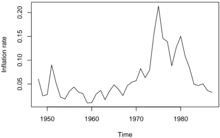
As a first step towards the estimation of an expectations-augmented Phillips curve (see Section 2.3), Bai and Perron model the post-war UK inflation rate, using annual data for the consumer price index (CPI) for the period 1947–1987. (We note that this amounts to using inflation rates for the period 1948–1987, although starting values for the year 1946 are available in the data set provided by Bai and Perron in the JAE data archive.) For this and the following example, Bai and Perron give the parameter settings for their results in their Tables II and III but do not provide a program containing the function calls tobrcode.src, rendering our task more difficult compared to the real interest data considered in the preceding section.
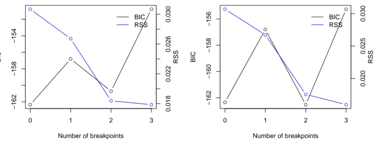
The model is a first-order autoregression, and the search for breakpoints utilizes a bandwidth of = 0.2, corresponding to a minimum segment size ofh= 8. This amounts to allowing for up to m∗= 3 breaks. Figure 3 presents the data and Figure 4 (left panel) presents the residual sum of squares and the BIC for all models with up to three breaks. Confirming Bai and Perron, the BIC selectsm = 0 breaks. However, the behavior of the BIC is somewhat erratic, it increases when moving from a zero-break to a one-break model and decreases when moving further to a two-break model. At the same time, the RSS rapidly decreases for models with up tom= 2 breaks, there is only a small decrease thereafter. This underlines the familiar problems with information criteria in dynamic models, as noted by Bai and Perron.
Following Bai and Perron, we now consider models with one and two breaks. For the former, we obtain a structural change in 1967, with an autoregressive parameter increasing from 0.274 to
Time
Inflation rate
1950 1960 1970 1980
0.050.100.150.20
Figure 3: UK inflation rate, 1948–1987.
Table III: UK CPI inflation rate (1948–1987) Parameter estimates with two breaks (h= 8) δˆ1,1 ˆδ1,2 δˆ1,3 Tˆ1 Tˆ2
0.025 -0.001 0.018 1967 1975
(0.008) (0.020) (0.016) 1965–1972 1973–1981 δˆ2,1 ˆδ2,2 δˆ2,3
0.274 1.343 0.683 (0.200) (0.250) (0.136)
Parameter estimates with two breaks (h= 7) δˆ1,1 ˆδ1,2 δˆ1,3 Tˆ1 Tˆ2
0.021 0.130 0.011 1973 1980
(0.008) (0.044) (0.006) 1969–1974 1979–1985 δˆ2,1 ˆδ2,2 δˆ2,3
0.488 0.115 0.633 (0.179) (0.312) (0.073)
0.739. These estimates are numerically identical to those reported by Bai and Perron and point to differences in the persistence of inflation. The intercept term is virtually unaffected, it being estimated at 0.025 before the break and at 0.024 thereafter (Bai and Perron do not report these estimates). However, the plot of the BIC and the RSS suggests that a two-break model is worth considering (Bai and Perron arrive at this conclusion on the grounds of various tests). Results for this model are presented in the upper part of Table III. It also has the breakpoint 1967, the additional break is at 1975.
It emerges that there are very minor differences in estimates of regression coefficients and their standard errors, the estimated break dates agree as well. However, there are again difficulties with the confidence intervals for the break dates. We have been unable to determine the exact source of the problem: after adjusting the lower endpoints as described in the preceding section our evaluations inRandGAUSS(usingbrcode.src) both yield the confidence intervals reported in Table III.
●
●
●
●
Number of breakpoints
BIC −162−158−154
●
●
●
●
BIC RSS
0.0180.0220.0260.030 RSS
0 1 2 3
●
●
●
●
Number of breakpoints BIC −162−160−158−156
●
●
●
●
BIC RSS
0.0200.0250.030 RSS
0 1 2 3
Figure 4: RSS and BIC for UK inflation data with up tom= 3 breaks forh= 8 (left) andh= 7 (right).
An issue worth exploring, although not directly relevant to a replication study, is the effect of the bandwidth parameter, h. Reducing hfrom 8 to 7 (or in fact any h ∈ {4, . . . ,7}), we arrive at a different model (with lower RSS) whose estimates are reported in the lower part of Table III.
RSS and BIC are depicted in the right panel of Figure 4, showing that a two-break model is the minimum BIC model. This time, the break dates are 1973 and 1980; they agree well with the Arab oil embargo following the Yom Kippur war and the Iran-Iraq war, respectively; events that are clearly most relevant to an inflation series.
For comparison, we also estimated this model inGAUSS using brcode.src, once more there were problems with one of the confidence intervals. While the first interval is identical in GAUSSand R, for the second interval only the lower limits agree. The upper limit is estimated at 1982 by GAUSS. Again, this is due to an underflow: a closer look reveals thatGAUSS v3.2.38 is not able to deliver quantiles below the 20% quantile.
2.3 Phillips curve
Finally, we consider the expectations-augmented Phillips curve, whose reduced form is
∆wt=γ1+γ2∆pt−1+γ3∆ut+γ4ut−1+ξt, (3) where wt is the logarithm of nominal wages,pt is the logarithm of the CPI, andutis the unem- ployment rate.
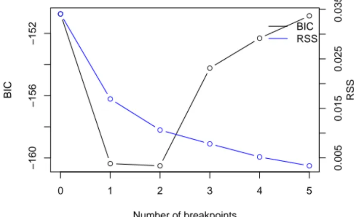
Using the data for the UK for the period 1948–1987 presented in the preceding section, Bai and Perron consider a partial structural change model arguing that changes in the inflation process should only affect coefficients γ1 and γ2 with no effect on coefficients γ3 and γ4. The current version ofstrucchangedoes not allow for partial structural change models, we therefore segment the full model usingh= 5 (larger than the Bai and Perron setting ofh= 3 because we lose extra degrees of freedom).
The BIC, depicted in Figure 5, yields a two-break model with changes in 1966 and 1974. These agree with the estimates of Bai and Perron, even the corresponding confidence intervals are almost identical, despite the fact that slightly different models are estimated. This indicates that there are no numerical problems with the computation of quantiles for this data set.
Since we are mainly interested in replication, we now proceed with estimating the partial structural change model given the estimated breakpoints. The results are presented in Table IV, they agree
●
● ●
●
●
●
Number of breakpoints
BIC −160−156−152
●
●
●
●
●
●
BIC RSS
0.0050.0150.0250.035 RSS
0 1 2 3 4 5
Figure 5: RSS and BIC for the Phillips curve equation.
Table IV: Phillips curve equation Parameter estimates with two breaks ˆ
γ1,1 γˆ1,2 ˆγ1,3 Tˆ1 Tˆ2
0.066 0.062 0.181 1967 1975
(0.012) (0.019) (0.054) 1966–1968 1974–1976 ˆ
γ2,1 γˆ2,2 ˆγ2,3
0.094 1.231 0.016 (0.241) (0.205) (0.257)
ˆ
γ3 ˆγ4
-0.144 -0.875 (0.582) (0.373)
rather well with those provided by Bai and Perron.
3. CONCLUSION
When we started with this project, we hoped that the results of Bai and Perron (2003) were easily replicated using ourRpackage. In fact, early versions ofstrucchangewere being developed when their paper was announced as forthcoming in the Journal of Applied Econometrics. When the JAE started its Replication Section in early 2003 (in the same issue in which the Bai and Perron paper was published), we felt that this paper provided an ideal opportunity to try out strucchange on other authors’ data. Since the JAE’s replication policy encourages the use of software packages different from those used for the original publication, our main goal was to describe our own package which offers a different approach to multiple structural change models in an object-oriented and open-source computing environment. However, things turned out to be more difficult when we tried to validate the confidence intervals. With some effort, we were able to trace these problems to an underflow problem that is not easy to overcome inGAUSS. Lessons are threefold:
Evidently, numerical accuracy is important. Vinod (2000) has reported on numerical problems in GAUSS related to more standard tasks. Here we encountered difficulties in connection with the quantiles of a nonstandard distribution. Naturally, problems of this type are bound to occur in all software environments, and only further replication studies will bring them to the attention of researchers and software developers. We note that terms of the type exp(x)·Φ(−√
x), with x
“large”, regularly occur in distribution theory pertaining to the estimation of breakpoints. In view of the recent interest in time series with multiple structural changes in econometric literature, the problem encountered here might therefore perhaps be more widespread and just has gone undetected so far.
We second McCullough and Vinod (2003) in suggesting journal archives with mandatory data and code. At present, the JAE only requires data, more often than not the corresponding code is not available. We are therefore grateful to Professors Bai and Perron for making their code publicly available without being obliged to. Without their code, this replication project would have had to stop halfway: GAUSS returns this, R returns that, and it would have been much harder to determine the source of the observed differences. With their code, we can confidently say that numerical problems inGAUSSare responsible for most of the differences.
Finally, as pointed out by McCullough and Vinod (2003), even data and code together will not be sufficient. In addition, anybody trying to replicate the results of some paper will require information on the software package including the version, the operating system and preferably the exact function calls to the package used in the analysis. Fortunately, there is a convenient way to achieve this (and more), at least for the combination of computing environment and text processor used by the authors of this paper,Rand LATEX. Rprovides the functionSweave(in the
toolspackage) which is able to perform computations on integrated text documents that mix code (in R) and corresponding documentation (in LATEX). The code can be extracted and executed to produce figures, tables and other output along with a standard LATEX file in which these are inserted. This LATEX file may subsequently be compiled in the usual way. Using this approach of dynamic documents with tightly coupled code and documentation, it is much easier to ensure that the data sets used, the programs employed, the results of computations and the description of these in the paper are always in sync—indeed, after changes to some part of the analysis the document just has to be recompiled. (In principle, it would also be possible to mix documentation and code from other languages but currently elaborate drivers appear to be only available for R and LATEX.) See Leisch (2003) for a detailed description of Sweaveand Leisch and Rossini (2003) for its use in connection with reviewing and replicating statistical research.
Computational details
Ris an interpreted language and mostly platform independent, hence the versions of Rand the packages used are more important than the architecture of the PC and the operating system used.
The results were obtained usingR1.8.1—with the packagesstrucchange1.2–2,sandwich0.1–2 and zoo 0.1–3—and were identical on various platforms including PCs running Debian GNU/Linux (with a 2.4–22 kernel) and Windows XP Professional, version 2002.
GAUSSv3.2.38 was run under Windows XP Professional, version 2002, on a 1.67 GHz AMD Athlon XP 2000+ processor.
Acknowledgements
The research of Achim Zeileis was supported by the Austrian Science Foundation (FWF) under grant SFB#010 (‘Adaptive Information Systems and Modeling in Economics and Management Science’).
The work of Christian Kleiber was supported by the Deutsche Forschungsgemeinschaft (DFG), Sonderforschungsbereich 475.
We are grateful to Pierre Perron for detailed comments on a previous version which led us to provide a more complete explanation of the source of the problem inGAUSS. We would also like to thank Matei Demetrescu, Uwe Hassler, Roman Liesenfeld, and Mark Trede for running our GAUSSprograms inGAUSSfor Windows v5.0.22, v5.0.25, and v6.0.8, showing that the numerical problems encountered inGAUSSv3.2.38 persist in more recent versions of that software package.
REFERENCES
Abramowitz M, Stegun IA. 1964. Handbook of Mathematical Functions. Washington, D.C.: U.S.
Government Printing Office.
Andrews DWK. 1993. Tests for parameter instability and structural change with unknown change point. Econometrica61: 821–856.
Andrews DWK, Ploberger W. 1994. Optimal tests when a nuisance parameter is present only under the alternative. Econometrica 62: 1383–1414.
Bai J. 1997. Estimation of a change point in multiple regression models. Review of Economics and Statistics 79: 551–563.
Bai J, Perron P. 1998. Estimating and testing linear models with multiple structural changes.
Econometrica 66: 47–78.
Bai J, Perron P. 2003. Computation and analysis of multiple structural change models. Journal of Applied Econometrics 18: 1–22.
Chambers JM, Hastie TJ. 1992. Statistical Models in S. London: Chapman & Hall.
Cody WJ. 1969. Rational Chebyshev approximations for the error function. Mathematics of Computation 22: 631–637.
Cribari-Neto F, Zarkos SG. 1999. R: Yet another econometric programming environment.Journal of Applied Econometrics 14: 319–329.
Feller W. 1968. An Introduction to Probability Theory and Its Applications, Vol. 1, 3rd ed. New York: John Wiley.
Kuan CM, Hornik K. 1995. The generalized fluctuation test: A unifying view. Econometric Reviews 14: 135–161.
Leisch F. 2003. Sweave and beyond: Computations on text documents. In Hornik K, Leisch F, Zeileis A (eds.) Proceedings of the 3rd International Workshop on Distributed Statistical Computing, Vienna, Austria. ISSN 1609-395X.
URLhttp://www.ci.tuwien.ac.at/Conferences/DSC-2003/Proceedings/
Leisch F, Rossini AJ. 2003. Reproducible statistical research. Chance 16: 46–50.
McCullough BD, Vinod HD. 2003. Verifying the solution from a nonlinear solver: A case study.
American Economic Review 93: 873–892.
Racine J, Hyndman R. 2002. Using R to teach econometrics. Journal of Applied Econometrics 17: 175–189.
RDevelopment Core Team. 2004. R: A Language and Environment for Statistical Computing. R Foundation for Statistical Computing, Vienna, Austria. ISBN 3-900051-00-3.
URLhttp://www.R-project.org/
Vinod HD. 2000. Review of GAUSS for Windows, including its numerical accuracy. Journal of Applied Econometrics 15: 211–220.
Wilkinson GN, Rogers CE. 1973. Symbolic description of factorial models for analysis of variance.
Applied Statistics 22: 392–399.
Zeileis A, Leisch F, Hornik K, Kleiber C. 2002. strucchange: An R package for testing for structural change in linear regression models. Journal of Statistical Software 7: 1–38.
URLhttp://www.jstatsoft.org/v07/i02/