SFB 823
Testing for structural breaks via ordinal pattern
dependence
Discussion Paper
Alexander Schnurr, Herold DehlingNr. 5/2015
Testing for Structural Breaks via Ordinal Pattern Dependence
Alexander Schnurr∗
Fakult¨at f¨ur Mathematik, Technische Universit¨at Dortmund and Herold Dehling∗
Fakult¨at f¨ur Mathematik, Ruhr-Universit¨at Bochum January 26, 2015
Abstract
We propose new concepts in order to analyze and model the dependence structure between two time series. Our methods rely exclusively on the order structure of the data points. Hence, the methods are stable under monotone transformations of the time series and robust against small perturbations or measurement errors. Ordinal pattern dependence can be characterized by four parameters. We propose estimators for these parameters, and we calculate their asymptotic distributions. Furthermore, we derive a test for structural breaks within the dependence structure. All results are supplemented by simulation studies and empirical examples.
For three consecutive data points attaining different values, there are six possibil- ities how their values can be ordered. These possibilities are called ordinal patterns.
Our first idea is simply to count the number of coincidences of patterns in both time series, and to compare this with the expected number in the case of independence. If we detect a lot of coincident patterns, this means that the up-and-down behavior is similar. Hence, our concept can be seen as a way to measure non-linear ‘correlation’.
We show in the last section, how to generalize the concept in order to capture various other kinds of dependence.
Keywords: Time series, limit theorems, near epoch dependence, non-linear correlation.
∗The authors gratefully acknowledge financial support of the DFG (German science Foundation) SFB 823: Statistical modeling of nonlinear dynamic processes (projects C3 and C5).
1 Introduction
In Schnurr (2014) the concept of positive/negative ordinal pattern dependence has been introduced. In an empirical study he has found evidence that dependence of this kind appears in real-world financial data. In the present article, we provide consistent estima- tors for the key parameters in ordinal pattern dependence, and we derive their asymptotic distribution. Furthermore, we present a test for structural breaks in the dependence struc- ture. The applicability of this test is emphasized both, by a simulation study as well as by a real world data example. Roughly speaking, positive (resp. negative) ordinal pattern dependence corresponds to a co-monotonic behavior (resp. an anti-monotonic behavior) of two time series. Sometimes an entirely different connection between time series might be given. By introducing certain distance functions on the space of ordinal patterns we get the flexibility to analyze various kinds of dependence. Within this more general framework we derive again limit theorems and a test for structural breaks.
Detecting changes in the dependence structure is an important issue in various areas of applications. Analyzing medical data, a change from a synchronous movement of two data sets to an asynchronous one might indicate a disease or e.g. a higher risk for a heart attack. In mathematical finance it is a typical strategy to diversify a portfolio in order to reduce the risk. This does only work, if the assets in the portfolio are not moving in the same direction all the time. Therefore, as soon as a strong co-movement is detected, it might be necessary to restructure the portfolio.
From an abstract point of view, the objects under consideration are two discretely observed stochastic processes (Xn)n∈Zand (Yn)n∈Z. In order to keep the notation simple, we will always useZas index set. Increments are denoted by (∆Xn)n∈Z, that is, ∆Xn :=Xn− Xn−1. Furthermore, h∈N is the number of consecutive increments under consideration.
The dependence is modeled and analyzed in terms of so called ‘ordinal patterns’. At first we extract the ordinal information of each time series. With h+ 1 consecutive data points x0, x1, ...xh (or random variables) we associate a permutation in the following way:
we order the values top-to-bottom and write down the indices describing that order. If h was four and we got the data (x0, x1, x2, x3, x4) = (2,4,1,7,3.5), the highest value is obtained at 3, the second highest at 1 and so on. We obtain the vector (3,1,4,0,2) which
carries the full ordinal information of the data points. This vector of indices is called the ordinal pattern of (x0, ..., xh). A mathematical definition of this concept is postponed to the subsequent section. There, it also becomes clear how to deal with coincident values within (x0, ..., xh). The reflected vector (−x0, ...,−xh) yields the inverse pattern, that is, read the permutation from right to left. In the next step we compare the probability (in model classes) respectively the relative frequency (in real data) of coincident patterns between the two time series. If the (estimated) probability of coincident patterns is much higher than it would be under the hypothetical case of independence, we say that the two time series admit a positive ordinal pattern dependence. In the context of negative dependence we analyze the appearance respectively the probability of reflected patterns. The degree of this dependence might change over time: we see below that structural breaks of this kind show up in the dependence between the S&P 500 and its corresponding volatility index.
Ordinal patterns have been introduced in order to analyze large noisy data sets which appear in neuro-science, medicine and finance (cf. Bandt and Pompe (2002), Keller et al.
(2007), Sinn et al. (2013)). In all of these articles only a single data set has been considered.
To our knowledge the present paper is the first approach to derive the technical framework in order to use ordinal patterns in the context of dependence structures and their structural breaks.
The advantages of the method include that the analysis is stable under monotone trans- formations of the state space. The ordinal structure is not destroyed by small perturbations of the data or by measurement errors. Furthermore, there are quick algorithms to analyze the relative frequencies of ordinal patterns in given data sets (cf. Keller et al. (2007), Sec- tion 1.4). Reducing the complexity and having efficient algorithms at hand are important advantages in the context of Big Data. Furthermore, let us emphasize that unlike other concepts which are based on classical correlation, we do not have to impose the existence of second moments. This allows us to consider a bigger variety of model classes.
The minimum assumption in order to carry out our analysis is that the time series under consideration are ordinal pattern stationary (of order h), that is, the probability for each pattern remains the same over time. In the sections on limit theorems we will have to be slightly more restrictive and have to impose stationarity of the underlying time-series.
Obviously stationarity of a time series implies stationary increments, which in turn implies ordinal pattern stationarity.
The paper is organized as follows: in Section 2 we present the rigorous definitions of the concepts under consideration. In particular we recall and extend the concept of ordinal pattern dependence. For the reader’s convenience we have decided to derive the test for structural breaks first for this classical setting. In order to show the applicability of the proposed test we consider financial index data. It is then a relatively simple task to generalize our results to the more general framework which is described in Section 3. There, we consider the new concept of average weighted ordinal pattern dependence.
Some technical proofs have been postponed to Section 4. In Section 5 we present a short conclusion.
From the practical point of view, our main results are the tests on structural breaks (cf. Theorem 2.7 and its corollary) and the generalization of the concept of ordinal pattern dependence (Section 3). In the theoretical part the limit theorems for all parameters under consideration, in particular for p, are most remarkable (cf. Corollary 2.6).
The notation we are using is mostly standard: vectors are column vectors and′ denotes a transposed vector or matrix. In defining new objects we write ‘:=’ where the object to be defined stands on the left-hand side. We write R+ for [0,∞).
2 Methodology
First we fix some notations and the basic setup. Afterwards we present limit theorems for the parameters under consideration as well as our test on structural breaks.
2.1 Definitions and General Framework
Let us begin with the formal definition of ordinal patterns: leth∈Nandx= (x0, x1, ..., xh)∈ Rh+1. The ordinal pattern of x is the unique permutation Π(x) = (r0, r1, ..., rh) ∈ Sh+1
such that
(i)xr0 ≥xr1 ≥...≥xrh and
(ii) rj−1 > rj if xrj−1 =xrj for j ∈ {1, ..., h}.
For an element π ∈ Sh+1, m(π) is the reflected permutation, that is, read the permutation from right to left.
Let us now introduce the main quantities under consideration:
p:=P
Π(Xn, Xn+1, ..., Xn+h) = Π(Yn, Yn+1, ..., Yn+h) q:=P
π∈Sh+1P
Π(Xn, Xn+1, ..., Xn+h) = π
·P
Π(Yn, Yn+1, ..., Yn+h) = π r:=P
Π(Xn, Xn+1, ..., Xn+h) =m Π(Yn, Yn+1, ..., Yn+h) s:=P
π∈Sh+1P
Π(Xn, Xn+1, ..., Xn+h) = π
·P
m(Π(Yn, Yn+1, ..., Yn+h)) =π
The time seriesX and Y exhibit a positive ordinal pattern dependence (ord⊕) of order h∈N and level α >0 if
p > α+q
and negative ordinal pattern dependence (ord⊖) of orderh ∈N and level β >0 if r > β+s.
Let us shortly comment on the intuition behind these concepts: we compare the proba- bility of coincident (resp. reflected) patterns in the time series{p, r}with the (hypothetical) case of independence {q, s}. In order to have a concept which is comparable to correlation and other notions which describe or measure dependence between time series, we introduce the following quantity
ord(X, Y) :=
p−q 1−q
+
−
r−s 1−s
+
(1) which is called thestandardized ordinal pattern coefficient. It has the following advantages:
we obtain values between -1 and 1, becoming -1 resp. 1 in appropriate cases: let Y be a monotone transformation of X whereX is a time series which admits at least two different patterns with positive probability. In this case
ord(X, Y) =
1−q 1−q
+
−
0−s 1−s
+
= 1 (q, s <1).
In generalqbecomes 1, only if the time seriesX andY both admit only one pattern πwith positive probability (which is then automatically 1). In this case we would set ord(X, Y) = 1, since this situation corresponds to a perfect co-movement. A similar statement holds true for s in the case of anti-monotonic behavior.
Using the standardized coefficient, the interesting parameters are still p and r. If the time series X and Y under consideration are stationary, q and s do not change over time also. Recall that we do not want to find structural breaks within one of the time series, but in their dependence structure. In the context of change-points respectively structural breaks within one data set cf. Sinn et al. (2012).
Remark 2.1. It is important to note that our method depends on the definition of ordinal patterns which is not unique in the literature. In each case permutations are used in order to describe the relative position of h+ 1 consecutive data points. Most of the time the definition which we have given above is used. In Sinn et al. (2012), however, time is inverted while Bandt and Shiha (2007) use an entirely different approach which they call
‘order patterns’. Using their definition, the reflected pattern is no longer derived by reading the original pattern σ from the right to the left, but by subtracting: (h+ 1, ..., h+ 1)−σ.
However, the quantities p and q are invariant under bijective transformations (that is:
renaming) of the ordinal patterns. Therefore, our results remain valid whichever definition is used.
Given the observations (x1, y1), . . . ,(xn, yn), we want to estimate the parametersp, q, r, s, and to test for structural breaks in the level of ordinal pattern dependence. In the subse- quent section, we will propose estimators and test statistics, and determine their asymptotic distribution, asntends to infinity. Readers who are only interested in the test for structural breaks and its applications might skip the next subsection.
2.2 Asymptotic Distribution of the Estimators of p
The natural estimator of the parameter p is the sample analogue ˆ
pn = 1 n
n−h
X
i=1
1{Π(Xi,...,Xi+h)=Π(Yi,...,Yi+h)}. (2) The asymptotic results in our paper require some assumptions regarding the dependence structure of the underlying process (Xi, Yi)i∈Z. Roughly speaking, our results hold if the process is ‘short range dependent’. Specifically, we will assume that (Xi, Yi)i∈Z is a func- tional of an absolutely regular process. This assumption is valid for many processes arising
in probability theory, statistics and analysis; see e.g. Borovkova, Burton and Dehling (2001) for a large class of examples.
For the reader’s convenience we recall the following concept: let (Ω,F, P) be a proba- bility space. Given two sub-σ-fields A,B ⊂ F, we define
β(A,B) = supX
i,j
|P(Ai∩Bj)−P(Ai)P(Bj)|,
where the sup is taken over all partitions A1, . . . , AI ∈ A of Ω, and over all partitions B1, . . . , BJ ∈ B of Ω. The stochastic process (Zi)i∈Z is called absolutely regular with coefficients (βm)m≥1, if
βm := sup
n∈Z
β(F−∞n ,Fn+m+1∞ )→0,
as m→ ∞. Here Fkl denotes theσ-field generated by the random variables Zk, . . . , Zl. Now we can state our main assumption. We will see below that it is very weak and that the class under consideration contains several interesting and relevant examples.
Let (Xi, Yi)i≥1be anR2-valued stationary process, and let (Zi)i∈Zbe a stationary process with values in some measurable space S. We say that (Xi, Yi)i≥1 is a functional of the process (Zi)i∈Z, if there exists a measurable functionf :SZ →R2 such that, for all k≥1,
(Xk, Yk) =f((Zk+i)i∈Z).
We call (Xi, Yi)i≥1 a 1-approximating functional with constants (am)m≥1, if for anym ≥1, there exists a function fm :S2m+1 →R2 such that (for everyi∈Z)
Ek(Xi, Yi)−fm(Zi−m, . . . , Zi+m)k ≤am. (3)
Note that, in the Econometrics literature 1-approximating functionals are called L1- near epoch dependent (NED). The following examples show the richness of the class under consideration. Recall that every causal ARM A(p, q) process can be written as anM A(∞) process (cf. Brockwell and Davis (1991) Example 3.2.3.).
Example 2.2. (i) Let (Xi)i≥1 be an M A(∞) process, that is, Xi =
∞
X
j=0
αjZi−j
where (αj)j≥0 are real-valued coefficients with P∞
i=jα2j <∞, and where (Zi)i∈Z is an i.i.d.
process with mean zero and finite variance. (Xi)i≥1 is a 1-approximating functional with coefficients am =
P∞
j=m+1α2j1/2
. Limit theorems for M A(∞) processes require that the sequence (am)m≥0 decreases to zero sufficiently fast. The minimal requirement is usually that the coefficients (αj)j≥0 are absolutely summable. If this condition is violated, the process may exhibit long range dependence, which is e.g. characterized by non-normal limits and by a scaling different from the usual √
n-scaling. Let us remark that ordinal pattern distributions in (a single) ARM Atime series have been investigated in Bandt and Shiha (2007) Section 6.
(ii) Consider the map T : [0,1]−→[0,1], defined by T(ω) = 2ω mod 1, i.e., T(ω) =
2ω if 0≤ω≤1/2 2ω−1 if 1/2< ω≤1.
This function is well known as the one-dimensional baker’s map in the theory of dynamical systems. Let g : [0,1] → R be a Lipschitz-continuous function, and define the stochastic process (Xn)n≥0 by
Xn(ω) = g(Tn(ω)).
This process was studied by Kac (1946), who established the central limit theorem for partial sums Pn
i=1Xi, under the assumption that g is a function of bounded variation.
The time series (Xn)n≥0 is a 1-approximating functional of an i.i.d. process (Zj)j∈Z with approximating constants am =kgkL/2m+1 where k·kL denotes the Lipschitz norm.
(iii) The continued fraction expansion provides an example from analysis that falls under the framework of the processes studied in this paper. It is well known that any ω ∈(0,1]
has a unique continued fraction expansion
ω = 1
a1+a 1
2+a 1
3+···
,
where the coefficients ai, i ≥ 1, are non-negative integers. Since these coefficients are functions of ω, we obtain a stochastic process (Zi)i≥1, defined on the probability space Ω = (0,1] by Zi(ω) = ai. If we equip (0,1] with the Gauß measure
µ((0, x]) = 1
log 2log(1 +x),
the process (Zi)i≥1 becomes a stationaryψ-mixing process. We can then study the process of remainders
Xn(ω) = 1
Zn(ω) + Z 1
n+1(ω)+ 1
Zn+2(ω)+···
.
The process (Xn)n≥1 is a 1-approximating functional of the process (Zi)i≥1, and thus the results of the present paper are applicable to this example.
Remark 2.3. At first glance, it might be a bit surprising that examples from the theory of dynamical systems are treated in an article which deals with the order structure of data. In fact, there is a close relationship between these two mathematical subjects: using ordinal patterns in the analysis of time series is equivalent to dividing the state-space into a finite number of pieces and using only the information in which piece the state is contained at a certain time. This is known as symbolic dynamics in the theory of dynamical systems.
Each of these pieces is assigned with a so called symbol. Hence, orbits of the dynamical system are turned into sequences of symbols (cf. Keller et al. (2007), Section 1.2).
Processes that are 1-approximating functionals of an absolutely regular process satisfy practically all limit theorems of probability theory, provided the 1-approximation coef- ficients am and the absolute regularity coefficients βk decrease sufficiently fast. In our applications below, we are not so much interested in limit theorems for the (Xi, Yi)-process itself, but in limit theorems for certain functions g((Xi, Yi), . . . ,(Xi+h, Yi+h)) of the data.
We then have to show that these functions are 1-approximating functionals, as well. We will now state this result for two functions that play a role in the context of the present research. A preliminary lemma, along with its proof, is postponed to Section 4.
Theorem 2.4. Let (Xi, Yi)i≥1 be a stationary 1-approximating functional of the absolutely regular process (Zi)i≥1. Let (β(k))k≥1 denote the mixing coefficients of the process (Zi)i≥1, and let (ak)k≥1 denote the 1-approximation constants. Assume that
∞
X
k=1
(√
ak+β(k))<∞. (4)
Furthermore, assume that the distribution functions of Xi−X1, and of Yi−Y1, are both Lipschitz-continuous, for any i∈ {1, . . . , h+ 1}. Then, as n → ∞,
√n(ˆpn−p)−→D N(0, σ2), (5)
where the asymptotic variance is given by the series
σ2 = Var(1{Π(X1,...,Xh+1)=Π(Y1,...,Yh+1)}) (6) +2
∞
X
m=2
Cov 1{Π(X1,...,Xh+1)=Π(Y1,...,Yh+1)},1{Π(Xm,...,Xm+h)=Π(Ym,...,Ym+h)}
,
Proof. We apply Theorem 18.6.3 of Ibragimov and Linnik (1971) to the partial sums of the random variables
ξi := 1{Π(Xi,...,Xi+h)=Π(Yi,...,Yi+h)}.
By Lemma 4.1, we get that ξi is a 1-approximating functional of the process (Zi)i≥1 with approximation constants (√ak)k≥1. Thus, the conditions of Theorem 18.6.3 of Ibragimov and Linnik (1971) are satisfied, and hence (5) holds.
Remark 2.5. Theorem 2.4 holds under the assumption that the underlying time series (Xi, Yi)i≥1 is short range dependent. In the case of long-range dependent time series, other limit theorems hold, albeit with a normalization that is different from the standard √
n- normalization.
In order to determine asymptotic confidence intervals for pusing the above limit theo- rem, we need to estimate the limit varianceσ2. De Jong and Davidson (2000) have proposed a kernel estimator for the series on the r.h.s. of (6). Let k : R → [0,1] be a symmetric kernel, i.e. k(−x) =k(x), that is continuous in 0 and safisfies k(0) = 1, and let (bn)n≥1 be a bandwidth sequence tending to infinity. Then we define the estimator
ˆ σn2 = 1
n
n−h
X
i=1 n−h
X
j=1
k i−j
bn
1{Π(Xi,...,Xi+h)=Π(Yi,...,Yi+h)}−pˆn
1{Π(Xj,...,Xj+h)=Π(Yj,...,Yj+h)}−pˆn
. (7) De Jong and Davidson (2000) show that ˆσn2 is a consistent estimator ofσ2, provided some technical conditions concerning the kernel function k, the bandwidth sequence (bn)n≥1 and the process (Xi, Yi)i≥1 hold. The assumptions on the process follow from our assumptions.
Concerning the kernel function and the bandwidth sequence, a possible choice is given by k(x) = (1− |x|)1[−1,1](x) and bn = log(n). We thus obtain the following corollary to Theorem 2.4.
Corollary 2.6. Under the same assumptions as in Theorem 2.4
√n(ˆpn−p) ˆ σn
−→D N(0,1).
As a consequence, [ˆpn−zασˆn,pˆn−zασˆn] is a confidence interval with asymptotic coverage probability(1−α). Herezα denotes the upperαquantile of the standard normal distribution.
We complement this theoretical result with a simulation of two correlated standard normal AR(1) time series, where the AR-parameter φ is 0.1. Furthermore we have set h = 2, p = 0.6353, n = 1000, k(x) and bn as above. We have simulated this 1000 times obtaining the following histogram and Q–Q plot.
Histogram of sqrt(n) * (p_n − 0.6353)/sigma_n
sqrt(n) * (p_n − 0.6353)/sigma_n
Density
−3 −2 −1 0 1 2 3
0.00.10.20.30.4
Figure 1: Histogram of √
n(ˆpn−p)/ˆσn for 1000 simulations of correlated AR(1) time series and density of N(0,1) distribution.
−3 −2 −1 0 1 2 3
−3−2−10123
Normal Q−Q Plot
Theoretical Quantiles
Sample Quantiles
Figure 2: Q–Q plot of √
n(ˆpn−p)/ˆσn for 1000 simulations of correlated AR(1) time series and N(0,1) distribution.
2.3 Structural Breaks
As we have pointed out above the interesting parameter, in order to detect structural breaks in the dependence structure, is p. Ifpchanges significantly over time,r has to change also.
Furthermore, in order to analyze rone can instead analyzepforX and−Y. For stationary time series, the values of q and s are stationary over time, too.
In order to test the hypothesis that there is no change in the ordinal pattern dependence, we propose the test statistic
Tn= max
0≤k≤n−h
√1 n
k
X
i=1
1{Π(Xi,...,Xi+h)=Π(Yi,...,Yi+h)}−pˆn
(8) and prove limit theorems which are valid under the hypothesis.
Theorem 2.7. Under the same assumptions as in Theorem 2.4, we have Tn
−→D σ sup
0≤λ≤1|W(λ)−λW(1)|,
where σ is defined in (6), and where (W(λ))0≤λ≤1 is standard Brownian motion.
The proof is again postponed to Section 4.
Corollary 2.8. Under the same assumptions as in Theorem 2.4, we have 1
ˆ σn
Tn D
−→ sup
0≤λ≤1|W(λ)−λW(1)|,
where σˆn is defined in (7), and where (W(λ))0≤λ≤1 is standard Brownian motion.
Remark 2.9. Note that the distribution of sup0≤λ≤1|W(λ)−λW(1)| is the Kolmogorov distribution. If we denote the upper α quantile of the Kolmogorov distribution by kα, the test that rejects the hypothesis of no change when Tn/ˆσn ≥kα has level α.
Example 2.10. Again we complement the theoretical result with a simulation study. In both cases we have simulated two correlated AR(1) time series, where the AR-parameter φ is 0.2. Furthermore we have set h = 2, n = 1000, k(x) and bn as above. In the first time series (Figure 3), there is no structural break (p= 0.6353). In the second time series (Figure 4) we have set p = 0.6353 for the first 500 data points and p = 0.5378 for the second 500 data points. We have simulated both pairs of time series 1000 times. Recall that the 0.95 quantile of the Kolmogorov distribution is 1.36.
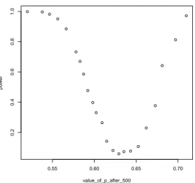
Let us, furthermore, analyze empirically the power of the test under different sizes of the change: we have used the same setting as above and obtain in Figure 5 the power of the test for various values of p after the break.
Histogram of T_n/sigma_n
T_n/sigma_n
Density
0.5 1.0 1.5 2.0
0.00.51.01.5
Figure 3: Histogram ofTn/ˆσnfor 1000 sim- ulations of correlated AR(1) time series without structural break and Kolmogorov density.
Histogram of T_n/sigma_n
T_n/sigma_n
Density
0 1 2 3 4
0.00.51.01.5
Figure 4: Histogram ofTn/ˆσnfor 1000 sim- ulations of correlated AR(1) time series with a change of p after 500 observations and Kolmogorov density
0.55 0.60 0.65 0.70
0.20.40.60.81.0
value_of_p_after_500
power
Figure 5: Empirical power of the test for structural breaks for different values of p after 500 data points.
We now work with simulated data sets which have been generated under three distinct settings: the normal distribution, the Student-t distribution with 2 degrees of freedom and the Cauchy distribution. For 500, 1000 and 2000 data points, we analyze structural breaks
after 1/4, 1/3 respectively 1/2 of the data. For the resultingAR(1)-time series withφ= 0.2 as above we analyze changes in pfrom 0.635 to 0.437.
n=500 n=1000 n=2000
break Normal Student-t Cauchy break Normal Student-t Cauchy break Normal Student-t Cauchy
125 0.628 0.611 0.559 250 0.938 0.891 0.861 500 0.998 0.998 0.996
167 0.776 0.769 0.71 333 0.979 0.973 0.958 667 1 0.999 1
250 0.877 0.851 0.81 500 0.997 0.992 0.984 1000 1 1 1
Let us emphasize that in medical and financial data n=2000 is a reasonable number which is often obtained. It is surprising that we get strong results even in the highly irregular Cauchy setting.
Finally, we use our method on real data.
Example 2.11. Let us consider the S&P 500 and its corresponding volatility Index VIX. We cannot go into the details of the Chicago Board Options Exchange Volatility Index (VIX), but we give a short overview: the index was introduced in 1993 in order to measure the US-market’s expectation of 30-day volatility which is implied by at-the-money S&P 100 option prices. Since 2003, the VIX is calculated based on S&P 500 data (we write SPX for short). The VIX is often qualified as the ‘fear index’ in newspapers, TV shows and also in research papers. It has been discussed whether the VIX is a self-fulfilling prophecy or if it is a good predictor for the future anyway (cf. Whaley (2008), and the references given therein). For us the following facts are of importance:
• The VIX can be used to measure the market volatility at the moment it is calculated (instead of trying to predict the future).
• Whether we use the S&P 100 or the S&P 500 data makes no difference, they are ‘for all intents and purposes (...) perfect substitutes’ (Whaley (2008), p.3).
• The relation between the two datasets (SPX↔VIX) is difficult to model (cf. Madan and Yor (2011)).
• There is a negative relation between the datasets which is asymmetric and hence, in particular, not linear (cf. Whaley (2008), Section IV).
We have used open source data which we have extracted from finance.yahoo.com. We have analyzed the daily ‘close prices’ for two periods of time each consisting in 2000 data
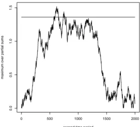
points for h= 2. In the time period from 1990-01-02 (the first day for which the VIX has been calculated) until 1997-11-25 we obtain T2000/ˆσ2000 = 0.843. In the time period from 1997-11-26 to 2005-11-08 we get T2000/ˆσ2000 = 1.5174. Hence, our test suggests that there has been a structural break in the dependence between the two time series in this second time period (level α = 0.05). Recall that the so called dot-com bubble falls in the second time period. The effect gets weaker as h increases. However, forh= 3 resp. h= 4 we still get significant results in case of the second time period, namely, T2000/ˆσ2000 is 1.4898 resp.
1.3616. Let us have a closer look on the values of
√1 nˆσn
k
X
i=1
1{Π(Xi,...,Xi+h)=Π(Yi,...,Yi+h)}−pˆn
before the maximum in (8) is taken. The vertical line is the 0.95-quantile of the Kolmogorov distribution.
0 500 1000 1500 2000
0.00.51.01.5
first time period
maximum over partial sums
Figure 6: No structural break is detected in the first 8 year period.
0 500 1000 1500 2000
0.00.51.01.5
second time period
maximum over partial sums
Figure 7: In the second time period a struc- tural break is detected.
2.4 Estimating the Other Parameters
Now we deal with the other parameters under consideration in order to estimate the stan- dardized ordinal pattern coefficient.
To estimate the parameter q, we define the following auxiliary parameters
qX(π) = P(Π(X1, . . . , Xh) =π) (9) qY(π) = P(Π(Y1, . . . , Yh) =π). (10) where π ∈Sh+1 denotes a permutation. Note that we have the following identity
q= X
π∈Sh
qX(π)qY(π).
We estimate the parameters qX(π) and qY(π) by their sample analogues ˆ
qX(π) = 1 n
n−h
X
i=1
1{π(Xi,...,Xi+h)=π} (11)
ˆ
qY(π) = 1 n
n−h
X
i=1
1{π(Yi,...,Yi+h)=π}, (12)
and finally q by the plug-in estimator ˆ
qn= X
π∈Sh
ˆ
qX(π) ˆqY(π). (13)
Theorem 2.12. Under the same conditions as in Theorem 2.4, the random vector
√n((ˆqX(π)−qX(π))π∈Sh,(ˆqY(π)−qY(π))π∈Sh)
converges in distribution to a multivariate normal distribution with mean vector zero and covariance matrix
Σ=
Σ11 Σ12
Σ12 Σ22
, where the entries of the (n!×n!) block matrices Σ11= σπ,π11′
π,π′∈Sh , Σ12 = σ12π,π′
π,π′∈Sh, and Σ22= σπ,π22′
π,π′∈Sh are given by the following formulas σπ,π11′ =
∞
X
k=−∞
Cov(1{π(X1,...,Xh)=π},1{π(Xk+1,...,Xk+h)=π′}) (14) σπ,π12′ =
∞
X
k=−∞
Cov(1{π(X1,...,Xh)=π},1{π(Yk+1,...,Yk+h)=π′}) (15) σπ,π22′ =
∞
X
k=−∞
Cov(1{π(Y1,...,Yh)=π},1{π(Yk+1,...,Yk+h)=π′}). (16)
Proof. This follows from the multivariate CLT for functionals of mixing processes, which can be derived from Theorem 18.6.3 of Ibragimov and Linnik (1971) by using the Cram´er- Wold device.
Remark 2.13. We have presented the formulas (14)–(16) for the asymptotic covariances for the case when the underlying process (Xk, Yk)k∈Z is two-sided. In the case of a one-sided process (Xk, Yk)k≥1, the formulas have to be adapted. E.g., in this case (14) becomes
σππ11′ = Cov(1{π(X1,...,Xh)=π},1{π(X1,...,Xh)=π′}) +
∞
X
k=1
Cov(1{π(X1,...,Xh)=π},1{π(Xk+1,...,Xk+h)=π′}) +
∞
X
k=1
Cov(1{π(X1,...,Xh)=π′},1{π(Xk+1,...,Xk+h)=π})
Using Theorem 2.12 and the delta method, we can now derive the asymptotic distribu- tion of the estimator ˆqn, defined in (13). The proof can be found in Section 4.
Theorem 2.14. Under the same assumptions as in Theorem 2.4,
√n(ˆqn−q)→N(0, γ2),
where the asymptotic variance γ2 is given by the formula γ2 = X
π,π′∈Sh
qY(π)σπ,π11′qY(π′) + 2 X
π,π′∈Sh
qX(π)σπ,π12′qY(π′) + X
π,π′∈Sh
qX(π)σπ,π22′qX(π′) If we want to apply the above limit theorems for hypothesis testing and the determi- nation of confidence intervals, we need to estimate the limit covariance matrix Σ. We will again apply the kernel estimate, proposed by De Jong and Davidson (2000), using the same kernel k and the same bandwidth (bn)n≥1 as before. We define the R2(h+1)!-valued random vectors
Vi =
1{π(Xi,...,Xi+h)=π}−qˆX(π)
π∈Sh+1, 1{π(Yi,...,Yi+h)=π}−qˆY(π)
π∈Sh+1
T
. The kernel estimator for the covariance matrix Σ is then given by
Σˆn= 1 n
n−h
X
i=1 n−h
X
j=1
k
i−j bn
ViVTj.