SFB 823
Testing for structural breaks in correlation: Does it improve Value-at-Risk forecasting?
Discussion Paper Tobias Berens, Gregor N. F. Weiß,
Dominik Wied
Nr. 21/2013
Testing for structural breaks in correlations:
Does it improve Value-at-Risk forecasting?
Tobias Berens
∗zeb/rolfes.schierenbeck.associates
Gregor N.F. Weiß
†Juniorprofessur Finance, Technische Universit¨at Dortmund
Dominik Wied
‡Juniorprofessur Finanz¨okonometrie, Technische Universit¨at Dortmund
May 15, 2013
Abstract In this paper, we compare the Constant Conditional Correlation (CCC) model to its dynamic counterpart, the Dynamic Conditional Correlation (DCC) model with respect to its accuracy for forecasting the Value-at-Risk of financial portfolios. Additionally, we modify these benchmark models by combining them with a pairwise test for constant correlations, a test for a constant correlation matrix, and a test for a constant covariance matrix. In an empirical horse race of these models based on five- and ten-dimensional portfolios, our study shows that the plain CCC- and DCC-GARCH models are outperformed in several settings by the approaches modified by tests for structural breaks in asset correlations and covariances.
Keywords: CCC-GARCH; DCC-GARCH; Estimation window; Structural breaks; VaR-forecast.
JEL Classification Numbers: C32, C41, C53, G17, G32.
Acknowledgement: Financial support by the Collaborative Research Center “Statistical Modeling of Non- linear Dynamic Processes” (SFB 823, project A1) of the German Research Foundation (DFG) is gratefully acknowledged.
∗Corresponding author; Address: Hammer Str. 165, D-48153 M¨unster, Germany, telephone: +49 251 97128 355, e-mail: tberens@zeb.de
†Address: Otto-Hahn-Str. 6a, D-44227 Dortmund, Germany, telephone: +49 231 755 4608, e-mail:
gregor.weiss@tu-dortmund.de
‡Address: CDI-Geb¨aude, D-44221 Dortmund, Germany, telephone: +49 231 755 5419, e-mail:
wied@statistik.tu-dortmund.de.
1 Introduction
It has become a stylized fact in the analysis of financial market data that correlations be- tween asset returns are time-varying. Bollerslev et al. (1988) were among the first to stress the importance of accounting for dynamic covariances in international asset pricing. Further empirical evidence for time-varying asset correlations is found by Longin and Solnik (1995) and Ang and Bekaert (2002) who show that correlations between international equity mar- kets increased over time and were higher in the high volatility regimes of bear markets.1 In response to these findings, studies in the field of financial econometrics in recent years have tried to model the dynamics in asset correlations. Most notably, Engle (2002) proposed the Dynamic Conditional Correlation (DCC) model that combines the flexibility of univariate generalized autoregressive conditional heteroskedasticity (GARCH) models but at the same time circumvents the necessity to estimate a large number of parameters. Further improve- ments of the flexibility of dynamic correlation models can then be achieved by testing for structural breaks in the correlation matrix of a given dataset and reestimating the dynamic model. Yet, the empirical literature still lacks a concise analysis of the question whether the increased flexibility of dynamic correlation models is needed for forecasting portfolio Value-at-Risk (VaR) accurately. Additionally, models that account for structural breaks in correlations could yield comparable accurate VaR-forecasts without imposing too strict assumptions on the dynamic behaviour of correlations over time.
In this paper, we investigate the question whether the Constant Conditional Correlation (CCC) model of Bollerslev (1990) is economically significantly outperformed with respect to its VaR-forecasting accuracy by competing models that account for the time-varying nature of asset correlations. To be precise, we compare the CCC model to its dynamic counter- part, the DCC model, introduced by Engle (2002), Engle and Sheppard (2001) (see also Tse and Tsui (2002)). Both models are then used in combination with recently proposed tests for structural breaks in a) the pairwise correlations, b) the correlation matrix and c)
1Evidence of correlations changing over time is also found by Pelletier (2006).
the covariance matrix of asset returns to yield a set of seven candidate models with a di- verse range of modeling flexibility.2 More precisely, we modify the plain CCC and DCC benchmark models by combining them with the pairwise test for constant correlations of Wied et al. (2012), the test for a constant correlation matrix of Wied (2012), and the test for a constant covariance matrix of Aue et al. (2009).3 The motivation for choosing these three tests lies in the fact that they are nonparametric and do not impose restrictive as- sumptions on the structure of the time series. We conduct a horse race of these models and compare their out-of-sample forecasting accuracy by using five- and ten-dimensional port- folios composed of European blue-chip stocks. The model performance is then assessed by performing formal backtests of VaR- and Expected Shortfall (ES)- forecasts using the un- conditional coverage test of Kupiec (1995), the CAViaR based test of Engle and Manganelli (2004) and Berkowitz et al. (2011), the ES backtest of McNeil and Frey (2000) and a back- test procedure based on the Basel guidelines for backtesting internal models.
The contributions of our paper are numerous and important. First, we propose the use of tests for structural breaks in correlations and covariances together with static and dynamic correlation-based models for forecasting the VaR of asset portfolios. Second, to the best knowledge of the authors, this study presents the first empirical analysis of the question whether static and dynamic correlation-based VaR-models can be improved by additionally testing for structural breaks in correlations. Third, we empirically test which of the tests for structural breaks (pairwise correlations, correlation matrix and covariance matrix) is best suited for capturing the dynamics in the returns on financial assets.
The paper proceeds as follows. In Section 2, we quickly review the standard GARCH(1,1) model we use as marginal models in our study. In Section 3, we discuss the multivariate dependence models as well as the tests for structural breaks in correlations used in our
2As the focus of our paper lies on the modeling of the dynamics in the dependence structure between assets, we do not consider structural breaks in the assets’ univariate volatilities. For a review of methods used for forecasting stock return volatility, see Poon and Granger (2003). Structural breaks in volatility are examined, for example, by Rapach and Strauss (2008).
3As we will explain later, the test of constant pairwise correlations cannot be combined with the DCC model. Therefore, only seven instead of eight models are compared in our study.
empirical study. Section 4 presents the data and outlines the test procedure of our empirical study. The results of the empirical study are presented in Section 5. Section 6 concludes.
2 Univariate GARCH model
GARCH-type models (see Bollerslev, 1986) have become the de-facto standard for describing the univariate behaviour of financial returns in a dynamic setting. The GARCH(1,1) model has been found to be the model of choice in the literature (see Hansen and Lunde, 2005).
Consequently, in the empirical study we opt for the simple GARCH(1,1) as the standard model to forecast the volatility of the univariate marginals.
Let rt,i denote the log-return of an asset i (i = 1, . . . , n) at time t (t = 0,1, . . . , T). Then the GARCH(1,1) process is defined by
rt,i = μi+t,i (1)
t,i = σt,izt,i (2)
σ2t,i = α0,i+α1,i2t−1,i+β1,iσt−1,i2 (3)
where α0,i > 0 and α1,i ≥ 0, β1,i ≥ 0 ensures a positive value of σt,i2 , and wide-sense stationarity requiresα1,i+β1,i <1. Along the lines of Bollerslev and Wooldridge (1992), the innovationszt,i follow a strict white noise process from a Student’s t distribution with mean 0, a scale parameter of 1, and ν > 2 degrees of freedom. After estimating the parameters of the univariate GARCH models with, for example, maximum likelihood, one-step-ahead forecasts for the conditional variances are simulated from equation (3) for each of thenassets in a portfolio separately via plug-in estimation of
σt+1,i2 =α0,i+α1,i2t,i+β1,iσ2t,i. (4)
3 Multivariate dependence models
In the following, the dependence models used in the empirical study are discussed. The selection includes five models employing statistical tests for the occurrence of structural breaks in the dependence structure and, for benchmarking purposes, the classical CCC- and DCC-GARCH models.
3.1 General setup of correlation-based dependence models
The general definition of a multivariate GARCH model with linear dependence can be written as
rt=μt+ Σ1/2t Zt (5)
wherertis a (n×1) vector of log returns,μtis a (n×1) vector ofE(rt) which we assume to be constant, and Σ1/2t is the Cholesky factor of a positive definite conditional covariance matrix Σtwhich corresponds to the variance σ2t in the univariate GARCH model. Furthermore, the innovationsZtcorrespond to zt,i of the univariate GARCH process and are assumed to come from a Student’s t distribution as described above. The conditional covariance matrix Σt can be expressed as
Σt =DtPtDt (6)
where Dt is a (n ×n) diagonal volatility matrix with the univariate conditional standard deviations σt,i derived from (3) as its diagonal entries and Pt = [ρt,ij] is a (n×n) positive definite correlation matrix where ρt,ii = 1 and |ρt,ij| < 1. From this it follows that the off-diagonal elements are defined as
[Σt]ij =σt,iσt,jρt,ij, i=j.
Our empirical study examines the one-step-ahead prediction of Value-at-Risk and Expected Shortfall. As we assumeμtto be constant, the prediction solely depends on the forecast of the
conditional covariance matrix Σt+1 =Dt+1Pt+1Dt+1. Note that in our case, estimation of the univariate variances takes place before estimating the correlation matrices. For this reason and since the forecasts of univariate variances are identical for all examined dependence models, divergences in the performance of VaR- and ES-prediction thus depend only on the selected model to forecast the correlation matrix Pt+1.
3.2 Constant and dynamic conditional correlation models
The Constant Conditional Correlation GARCH model by Bollerslev (1990) constitutes a basic concept to specify the dependence structure of a given data set, since the conditional correlations are assumed to be constant over time. Let Σt be the conditional covariance matrix in a CCC-GARCH(1,1) process at time t. Corresponding to equations (5) and (6), the one-step-ahead forecast of the conditional covariance matrix can be obtained by a plug- in estimation of Σt+1 = Dt+1PcDt+1. The correlation matrix Pc is assumed to be constant over time and its entries can be estimated with the arithmetic mean of products of the standardized residuals ˆzt,i (see Bollerslev, 1990, for details). Here, ˆzt,i = ˆt,iσˆt,i−1, where ˆσt,i is the (plug-in-) estimated conditional standard deviation based on (3) and ˆt,i = rti −μˆi. Dt+1 is determined by the univariate conditional variances σt+1,i2 obtained from (4) which are estimated by the plug-in method. The simplification of a constant dependence structure makes the model quite easy to estimate, in particular for high-dimensional portfolios. Due to its relatively simple design and its lasting popularity in the financial industry, we use the CCC-GARCH model as a useful benchmark.
Several studies starting with the seminal work by Longin and Solnik (1995) show that cor- relations of asset returns are not constant over time. Therefore, as a generalization of the CCC-GARCH model, Engle (2002) and Engle and Sheppard (2001) propose the Dynamic Conditional Correlation (DCC) GARCH model which allows the conditional correlation ma- trix to vary over time. The conditional covariance matrix is decomposed into conditional standard deviations and a correlation matrix via Σt=DtPtDt. The correlation matrix Pt is
assumed to be time-varying and is defined as
Pt=Q∗−1t QtQ∗−1t . (7)
The time-varying character of the DCC-GARCH model is implemented by
Qt= (1−α−β) ¯Q+α(zt−1zTt−1) +βQt−1. (8)
Q∗t is a diagonal matrix composed of the square root of the diagonal elements of Qt and Q¯ is the unconditional covariance matrix of the innovations zt−1,i. The DCC parameters have to satisfy α≤1, β ≤1 and α+β <1. The one-step-ahead forecast of the conditional covariance matrix can then be obtained as a plug-in estimator of Σt+1 =Dt+1Pt+1Dt+1. Here, Dt+1 is determined by the univariate conditional variances σ2t+1,i obtained from (4) and the conditional correlation matrix Pt+1 is determined by Qt+1 = (1−α−β) ¯Q+α(ztzTt) +βQt derived from (8). For details concerning the (maximum-likelihood) estimation ofPt, we refer to Engle (2002).
3.3 Tests for structural breaks in the dependence
In general, correlation based GARCH models can be extended by allowing for structural breaks in the dependence measure. We employ three recently proposed tests to detect structural breaks in P as well as in Σ and reestimate P after each change point. The basic motivation for using these tests is the fact that we want to know which data of the past we can use for estimating the correlation or covariance matrix. All three tests basically have the same structure: One compares the successively estimated quantities (bivariate correlations, correlation matrix, covariance matrix) with the corresponding quantities estimated from the whole sample and rejects the null of no-change if the difference becomes too large over time.
All three tests work under mild conditions on the time series which makes them applicable to financial data. They are nonparametric in the sense that one does not need to assume a
particular distribution such as a specific copula model or the normal distribution. Moreover, the tests allow for some serial dependence such that it is possible to apply the test on, for example, GARCH models. Principally, weak-sense stationarity is required for applying the fluctuation tests. While this is fulfilled in GARCH models under certain conditions, conditional heteroscedasticity might be a problem for the correlation tests as the tests might reject the null too often. To circumvent this problem, one can apply some kind of pre- filtering on the data. One potential drawback is the fact that it is a necessary condition to have finite fourth moments for deriving the asymptotic null distributions of the tests. While there is some evidence that second moments do exist in financial return data, the existence of finite fourth moments is doubtful. Nevertheless, we consider the fluctuation test to be applicable on returns as well. In the following, we will shortly present each test together with its respective null distributions.
3.3.1 Pairwise test for constant correlation
Wied et al. (2012) propose a fluctuation test for constant bivariate correlations. The test compares the successively estimated bivariate correlation coefficients with the correlation coefficient from the whole sample. The test statistic is given by
Dˆ max
2≤j≤T
√j
T|ρˆj −ρˆT|, (9)
where ˆD is an estimator described in Wied et al. (2012) that captures serial dependence and fluctuations of higher moments and serves for standardization. Also, the factor √j
T
serves for standardization, meaning that it compensates for the fact that correlations are in general better estimated for larger time series. The null hypothesis of constant correlation is rejected for too large values of the test statistic. Since the correlation test is designed for a bivariate vector, we control each entry of the population correlation matrix separately with this test. That means, we determine for each entry separately which data is used for its
estimation. Under the null hypothesis of constant correlation, the test statistic converges to sup0≤z≤1|B(z)|, where B is a one-dimensional standard Brownian bridge. Under a sequence of local alternatives, the test statistic converges against sup0≤z≤1|B(z) +C(z)|, where C is a deterministic function.
3.3.2 Test for a constant multivariate correlation matrix
Wied (2012) proposes an extension of the bivariate correlation test to a d-dimensional cor- relation matrix. The test statistic in this case is rather similar to the former case with the difference that one does not just consider one deviation
|ρˆj −ρˆT|,
but the sum over all “bivariate deviations”, that means,
1≤i,j≤p,i=j
√k T
ρˆijk −ρˆijT.
Also, the estimator ˆD is calculated differently. While the bivariate test uses a kernel-based estimator, the multivariate test uses a block bootstrap estimator, see Wied (2012) for details.
Under the null hypothesis of a constant correlation matrix, the test statistic converges to sup0≤z≤1d(d−1)/2
i=1 |Bi(z)|, where (Bi(z), z ∈ [0,1]), i = 1, . . . , d(d−1)/2 are independent standard Brownian bridges. Under local alternatives, we have convergence results that are similar to the ones with the former test.
3.3.3 Test for a constant multivariate covariance matrix
Aue et al. (2009) present a nonparametric fluctuation test for a constant d-dimensional co- variance matrix of the random vectors X1, . . . , XT with Xj = (Xj,1, . . . , Xj,d). Let vech(·) denote the operator which stacks the columns on and below the diagonal of a d×d matrix
into a vector and let A be the transpose of a matrixA. At first, we consider the term
Sj = j
√T
1 j
j
l=1
vech(XlXl)− 1 T
T
l=1
vech(XlXl)
,
for 1≤j ≤T, which measures the fluctuations of the estimated covariance matrices. Here, the factor √j
T again serves for standardization for the same reasons as described above.
The test statistic is then defined as max1≤j≤T SjESˆ j, where ˆE is an estimator which has the same structure as in the bivariate correlation test and is described in more detail in Aue et al. (2009). The limit distribution under the null hypothesis is the distribution of
sup
0≤z≤1
d(d+1)/2
i=1
Bi2(z),
where (Bi(z), z ∈[0,1]), i= 1, . . . , d(d+ 1)/2 are independent Brownian bridges.
Aue et al. (2009) show that the test is consistent against fixed alternatives. Note that the application of the test requires the assumption of constant first moments of the random vectors of the time series. The asymptotic result is derived under the assumption of zero expectation; if we had constant non-zero expectation, it would be necessary to subtract the arithmetic mean calculated from all observations from the original data which does not change the asymptotic distribution.
4 Data and test procedure
Our empirical study is designed as follows:
(1) Data and portfolio composition: We compute log returns by using daily total return quotes of stocks listed on the indices DAX30, CAC40, and FTSE100. With respect to each index, we build one 5-dimensional and one 10-dimensional portfolio of equal weighted assets. For the 5-dimensional (10-dimensional) portfolios we select those five (ten) companies which possess the highest index weighting on June 30, 2012 and meet the
requirement of a complete data history. The data set for each of the portfolios contains log returns of 4,970 trading days (we exclude non-trading days from our sample). The quotes cover a period from the autumn of 1992 to June 30, 2012. All quotes are obtained from Thomson Reuters Financial Datastream.
(2) Univariate modeling: To forecast the volatility of each asset in each portfolio at day t+ 1, GARCH(1,1) models are fitted to a moving time window consisting of the 1,000 preceding log returns. The use of a moving time window of 1,000 days is common in the literature and is in line with, e.g., McNeil et al. (2005) and Kuester et al. (2006).
Next, a one-step-ahead volatility forecast σt+1,i is computed by the use of the estimated GARCH parametersα0, α1 and β1 according to (4). Furthermore, degrees of freedom of the marginals are held to be constant atνc = 10.
(3) Testing for structural breaks and multivariate modeling: The correlations Pc and Pt of the plain CCC and DCC models are fitted to a sample consisting of the standardized residuals obtained from the univariate GARCH estimation. Therefore, the sample includes a moving time-window of 1,000 trading days preceding the forecast day t+ 1. We opt for a moving time window rather than for a fixed time-window, because a fixed time-window does not account for any changes in the correlation structure. As a second alternative, an expanding time-window could be used which is determined by a fixed starting point and a moving end. However, we do not use such a time-window, because the weighting of more recent data for the parameter fitting decreases when the time-window increases over time. In conclusion, the moving time-window approach allows the estimated parameter to change and therefore it is a benchmark which is hard to beat.
The estimation of the CCC and DCC parameters in combination with each of the three different tests for structural breaks is designed as follows. Similar to Wied (2013), we apply the structural break tests to the standardized residuals ˆzt,i of a moving time-
window of a constant length at each point in time t. Here, ˆzt,i = ˆt,iσˆt,i−1, where ˆσt,i is the (plug-in-) estimated conditional standard deviation based on (3) and ˆt,i =rti−μˆi. For the purpose of this study, the time-window consists of 1,000 trading days preceding the forecast day t + 1. In order to decide at which point in time a possible change occurs we use an algorithm based on Galeano and Wied (2013). First, within the sample of 1,000 trading days we identify the data point at which the test statistic takes its maximum. If this maximum is equal to or above the critical value, the null of a constant correlation/covariance is rejected.4 In this case, the data point is a natural estimator of a so called dominating change point. Second, at this point we split the sample into two parts and search for possible change points again in the latter part of the sample. The procedure stops if no new change point is detected. Finally, the constant correlation coefficientPc and the time-varying correlation coefficientPtare estimated on the basis the standardized residuals of a subsample, which starts at the day of the latest detected change point and ends at dayt. The sample size for estimatingP is limited to [100, . . . ,1,000]. Because we perform the tests on a daily basis, the nominal significance level might not be attained. Following Wied (2013), we do not address this topic within this study as we simply use the decisions of the tests in an explorative way. Note that in case of the application of the pairwise test for constant correlations this procedure is conducted for each of the off-diagonal elements of the correlation matrix. Because the resulting subsamples for each element are typically of different lengths, the estimation of DCC parameters is not feasible. Therefore, this test is only applied in combination with the CCC-GARCH model.
Concerning the test for a constant covariance matrix, Aue et al. (2009) approximate asymptotic critical values by simulating Brownian bridges on a fine grid. Wied et al.
4The critical values are computed for a significance level of 5% for each of the three structural break tests. We also tested a setup including a significance level of 1%. However, the forecasting results tend to be slightly worse. With respect to the test for a constant correlation matrix, we use a bootstrap approximation for a normalizing constant in order to approximate the asymptotic limit distribution of the test statistic. In line with Wied (2012), we chose 199 bootstrap replications.
(2013) show that for a small sample size this approach leads to considerably overesti- mated critical values and hence to very infrequent rejections. To this end, based on Wied et al. (2013), we simulate d-dimensional samples of standard normal distributed random variables representing 1,000 trading days. This sample size corresponds to the size of the moving time-window as explained above. After that, we compute the test statistic for the sample. We repeat this procedure 10,000 times. Finally, we determine the critical value by computing the 95%-quantile of the resulting test statistics. In ad- dition, we verify whether the asymptotic critical values used for the pairwise test for constant correlation and the test for a constant correlation matrix are suitable for finite samples including 1,000 trading days. To this end, we obtain critical values based on the procedure explained above and compare these to the corresponding asymptotic critical values. As shown in Table 1, in contrast to the differences for the test for a constant co- variance matrix, the differences corresponding to the two tests for constant correlations are in an acceptable range.
— Insert Table 1 about here —
(4) Simulations: For calculating VaR and ES, we do not use analytical methods but simu- lations as it is done, e.g., by Giot and Laurent (2003) and Alexander and Sheedy (2008).
For each of the n assets in a portfolio and for each day t, K = 100,000 random simu- lations5 of Student’s t-distributed log returns rt1(k), . . . , rtn(k) are generated by use of the mean μt, the univariate volatility forecast σt+1,i, the correlation matrix P as estimated by the models described in Section 3, and the degrees of freedom νc = 10.
(5) Estimation of VaR and ES: The daily VaR at the 100(1−α)% confidence level is computed from smoothed simulated log returns.6 The simulated log returns are first
5Giot and Laurent (2003) state that the choice of 100,000 simulations provides accurate estimates of the quantile.
6Pritsker (2006) show that the use of the (discrete) empirical cdf in Historical Simulation of VaR can lead to severely biased risk estimates.
smoothed by using the Epanechnikov kernel. The daily VaR at the 100(1−α)% con- fidence level is then given by the α-quantile of the kernel density estimate. To analyze the effect of different levels of significance on the quality of our models’ risk estimates, we set α = 0.05 and α = 0.01 and compare the results for the VaR-estimates with the realized portfolio losses in order to identify VaR-exceedances.
As the Value-at-Risk is not in general coherent, we also estimate the portfolios’ Expected Shortfalls which are given by
ESα(X) = E[X|X ≤V aRα(X)]. (10)
For dayt+ 1, we determine theESαby computing the mean of the simulated log returns below the estimated V aRα for that day.
(6) Backtesting and performance measurement: The performances of the different models are evaluated by applying appropriate backtests on the VaR- and ES- forecasts.
Since the univariate volatility forecasts for each of the VaR models are equal. Hence, differences in VaR-forecasts and VaR-violations can only result from differences in the estimated correlations. We employ the commonly used test of Kupiec (1995) to eval- uate whether the observed number of VaR-violations is consistent with the expected frequency (unconditional coverage). In addition, we take a look at the distribution of the VaR-violations. The day on which a VaR-violation occurs should be unpredictable, i.e., the violation-series should follow a martingale difference process. To this end, we perform the CAViaR-Test of Engle and Manganelli (2004) and Berkowitz et al. (2011).
The test is based on the idea that any transformation of the variables available when VaR is computed should not be correlated with the current violation. Consider the autoregression
It=α+
n
k=1
β1kIt−k+
n
k=1
β2kg(It−k, It−k−1,· · · , Rt−k, Rt−k−1,· · ·) +ut. (11)
In line with Berkowitz et al. (2011), we set g(It−k, It−k−1,· · · , Rt−k, Rt−k−1,· · ·) =
V aRt−k+1 and n = 1. The null hypothesis of a correctly specified model with
β1k = β2k = 0 is tested with a likelihood ratio test. The test statistic is asymptoti- cally χ2 distributed with two degrees of freedom. Berkowitz et al. (2011) evaluate the finite-sample size and power properties of various different VaR-backtests by conducting a Monte Carlo study where the return generating processes are based on real life data.
They find that the CAViaR-test shows a superior performance compared to competing models.
The Expected Shortfall is backtested with the test of McNeil and Frey (2000). This test evaluates the mean of the shortfall violations, i.e., the deviation of the realized shortfall against the ES in the case of a VaR-violation. The average error should be zero. The backtest is a one-sided test against the alternative hypothesis that the residuals have mean greater than zero or, equivalently, that the expected shortfall is systematically underestimated.
In addition to the statistical backtests, we assess the performance of the models from a practitioner’s point of view. According to the framework for backtesting internal models proposed by the Basel Commitee on Banking Supervision (1996), we measure the number of VaR-violations on a quarterly basis using the most recent twelve months of data. To be more precisely, we count the number of violations after every 60 trading days using the data of the most recent 250 trading days. We sum up the VaR-violations for each interval [1, . . . ,250], [61, . . . ,310],. . . , [3,721, . . . ,3,970]. This procedure leads to 63 results of one-year VaR-violation frequencies. Because we focus on the adaptability of a VaR model due to changes in correlations, we measure fluctuations in terms of the standard deviation of the 63 one-year VaR-violation frequencies.7 The standard deviation of a model which adapts well to these changes should be smaller than the
7This approach is based on McNeil et al. (2005), p. 58, where several VaR estimation methods are compared by computing the average absolute discrepancy per year between observed and expected numbers of VaR-violations. Here, we use the standard deviation rather than the average absolute discrepancy.
standard deviation of a less flexible model. We abstain from using the calculation of capital requirements according to the Basel guidelines to evaluate the performance of the different models. Da Veiga et al. (2011) find that using models which underestimate the VaR lead to low capital charges because the current penalty structure for excessive violations is not severe enough. For this reason, we consider the capital requirement not to be an appropriate performance measure.
5 Results
In this section, the results of our empirical study are discussed focusing on the specified aspects mentioned in the introduction of this paper.
5.1 Total Number of VaR Violations
We start the discussion of our results with the analysis of the total number of VaR-violations.
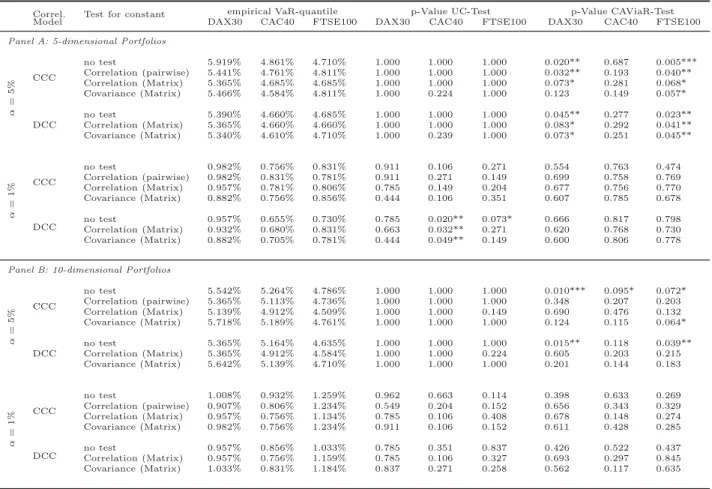
A key requirement with regard to VaR-forecasting models is that the number of VaR- violations should match the expected number related to the selected α-quantile. For each of the different models, we compute the empirical VaR-quantile by dividing the number of VaR-violations by the total number of 3,970 VaR-forecasts. Furthermore, we apply the un- conditional coverage test of Kupiec (1995) to test the null hypothesis of a correctly specified model. The results are reported in Table 2.
— Insert Table 2 about here —
With respect to the α = 5% quantile and the corresponding empirical VaR-quantiles, the majority of the results are in a narrow range around the target level. Only the VaR-forecasts for the DAX30 portfolios underestimate portfolio risk to some degree, whereby the models including the tests for structural breaks in the correlation as well as the DCC-GARCH model improve upon a plain CCC-GARCH model.
Furthermore, the application of the unconditional coverage test of Kupiec (1995) leads to p-values above the 10% threshold for statistical significance in the case of all approaches and all portfolios. For the α = 1% quantile, the empirical VaR-quantiles vary between 0.655%
and 1.259%. In particular, for the CAC40 portfolios, the empirical VaR-quantiles for each of the analyzed models are below the α-quantile. In several cases, this leads to a p-value below a significance level of 10%.
Because of the rare occurrence of statistically significant p-values, it is difficult to derive conclusions from the unconditional coverage test for a specific VaR-forecasting model. Each of them are more or less suitable for the underlying datasets. Consequently, to carve out the specific characteristics of the different models, a deeper analysis into the distribution of the VaR-exceedances is needed.
5.2 Distribution of VaR Violations
The total number of VaR-violations is not a sufficient criterion to evaluate the fit of the analyzed dependence models, because it gives no indication about the distribution of the VaR-violations. Among others, Longin and Solnik (2001) as well as Campbell et al. (2002) show that in particular in volatile bear markets correlations tend to increase. Consequently, in times where an effective risk management is most needed, inflexible dependence models may not be able to adequately adapt to changes in the dependence structure. This could lead to the undesired occurrence of clustered VaR-violations which in turn could lead to disastrous losses. To this end, we perform the CAViaR-based backtest of Engle and Manganelli (2004) and Berkowitz et al. (2011) to analyze the performance of the models used in our empirical study.
The results of the CAViaR test are presented in Table 2. Due to the six different portfolios and the two α-quantiles, we compute twelve p-values for each of the analyzed models. In summary, for each of the models combining the CCC- and DCC-GARCH approach with tests for structural breaks, the p-values fall short of the 10% threshold for statistical significance
in only two out of twelve cases. In contrast, the p-values of the plain CCC- and DCC- GARCH models are below a significance level of 10% in five and four cases, respectively.
It is noteworthy that all of the significant p-values are found for the 5% α-quantile. With respect to the 1% α-quantile, the CAViaR test does not lead to any statistical significant results. These results indicate that the additional use of the tests for structural breaks at least to some degree leads to less clustered VaR-violations for the 5% VaR.
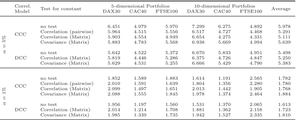
In addition to the statistical tests, we evaluate the performance of the different VaR- forecasting models from a perspective which is more relevant in practical terms. As explained in section 4, we follow the Basel guidelines for backtesting internal models and count the number of VaR-violations after every 60 trading days using the data of the preceding 250 trading days. Based on the resulting 63 quarterly VaR-violation frequencies, we compute standard deviations which are presented in Table 3.
— Insert Table 3 about here —
We start with the backtests for the α = 5% quantile. The CCC-GARCH models in combi- nation with structural break tests show lower standard deviations compared to their plain counterpart. In particular, the CCC-GARCH model in combination with the test for a constant correlation matrix leads to less clustered VaR-violations, regardless of the port- folio dimension. There are only small differences in the average standard deviation of the DCC-GARCH based models. However, the models which include tests for structural breaks improve slightly on the plain DCC-GARCH.
Continuing with the results for the α= 1% quantile, the average standard deviation ranges from 1.613 for the plain DCC-GARCH model to 1.884 for the CCC-GARCH model in com- bination with the test for a constant covariance matrix. The small differences of the results do not yield any evidence that one of the analyzed models is clearly preferable.
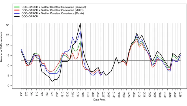
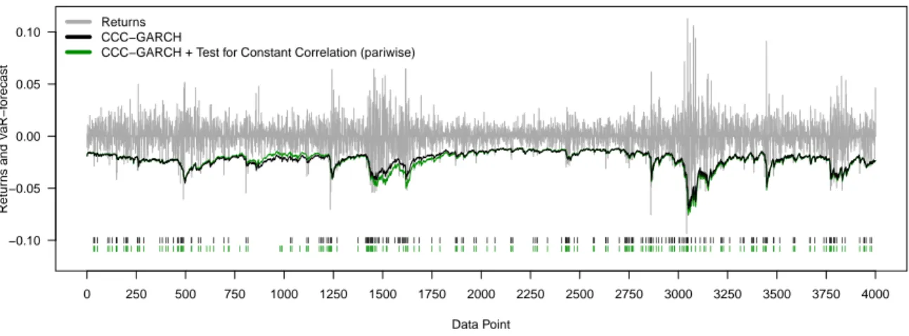
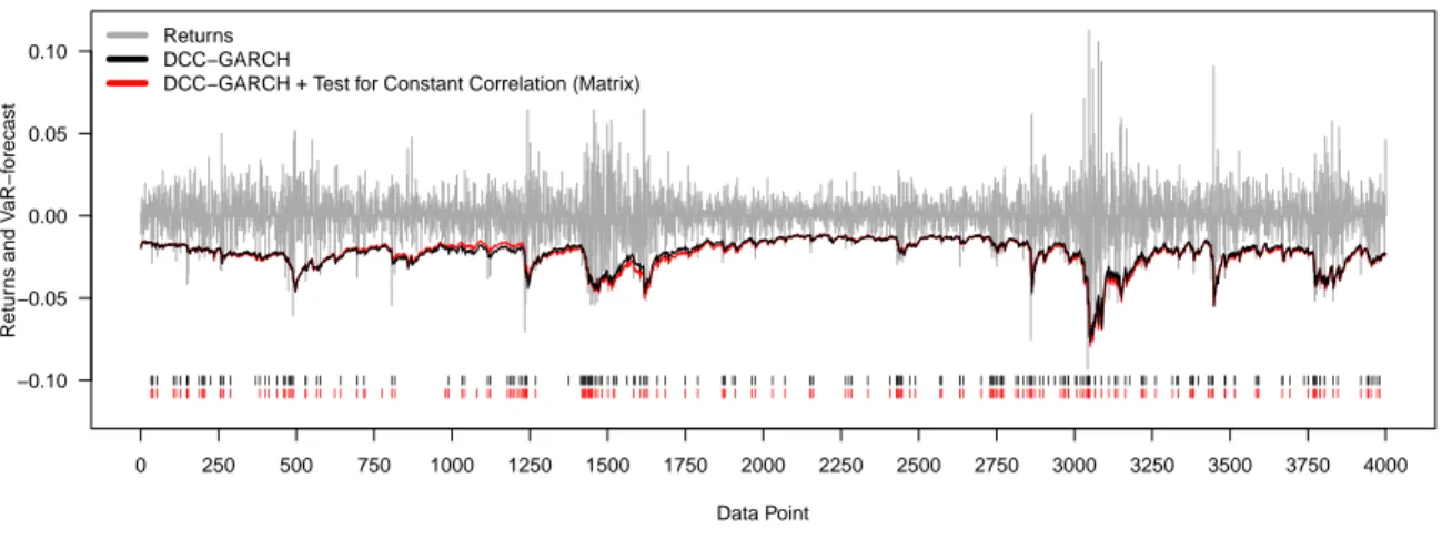
Because the (averaged) standard deviations of quarterly VaR-violation frequency is a highly aggregated performance measure, we analyze the effects of the application of tests for structural breaks by analyzing the VaR-exceedances for the α = 5% quantile using the
10-dimensional CAC40 portfolio as an example. Figure 1 illustrates the number of VaR- violations on a 60 trading day basis using the data of the most recent 250 trading days.
— Insert Figure 1 about here —
The VaR-violation frequency of the plain CCC- and DCC-GARCH models deviate from the required level in particular during four specific periods:
a) at the later stage of the dot-com bubble between the data points 730 (October 28, 1999) and 1,150 (June 27, 2001);
b) at the bear market after the burst of the dot-com bubble and the 9/11 attacks between the data points 1,450 (August 30, 2002) and 1,690 (August 11, 2003);
c) at the economic recovery between the data points 1,810 (January 29, 2004) and 2,410 (May 30, 2006);
d) and at the financial crisis between the data points 2,770 (October 24, 2007) and 3,250 (September 11, 2009).
To facilitate the analysis of the results, Figures 2 and 3 show the corresponding portfolio returns and daily VaR-forecasts of the CCC- and DCC-GARCH based models.
— Insert Figure 2 about here —
— Insert Figure 3 about here —
Turning to period a), the number of VaR-exceedances of the plain CCC- and DCC-GARCH models is far too low. The implementation of the structural break tests results in VaR- forecasts which are less conservative to some degree and therefore more accurate. Conse- quently, the additional use of these tests leads to a reduction of the extent by which the violation frequency falls short of the expected level. In contrast, during periods b) and d), the plain models show far too many exceedances, whereas the number of VaR-violations of the structural break test models are significantly lower. This applies particularly to the models in combination with the tests for constant correlations whose daily VaR-forecasts are distinctly more conservative. However, during the calm stock markets of period c), the daily
VaR-forecasts of the different models show hardly any different results. Nevertheless, the plain CCC- and DCC-GARCH models show a slightly lower degree of risk-overestimation compared to the remaining approaches.
5.3 Expected Shortfall
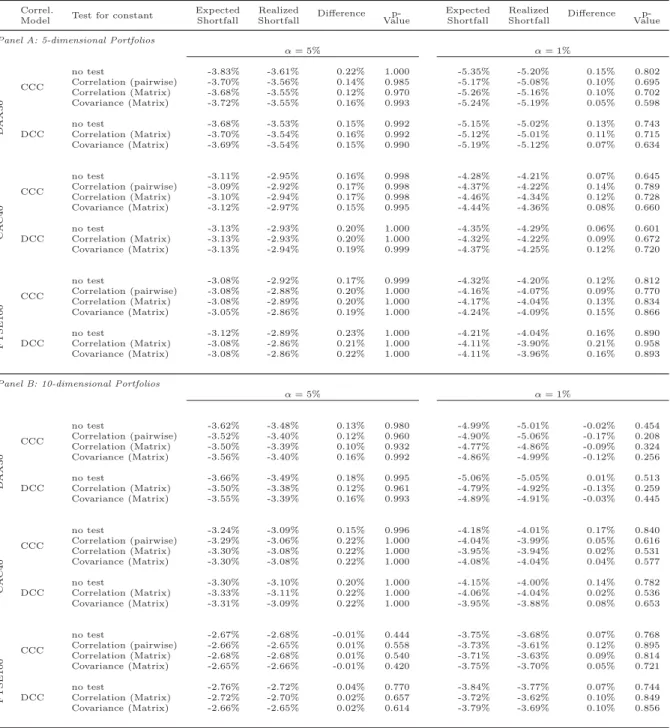
In addition to the measurement of the Value-at-Risk, we evaluate the different risk-models with respect to their accuracy in forecasting Expected Shortfall. To this end, we compare the models on the basis of the deviation of the realized shortfall against the ES in the case of a VaR-violation. Furthermore, we apply the backtest of McNeil and Frey (2000). The results are presented in Table 4.
— Insert Table 4 about here —
Overall, the realized shortfall of the models show only small deviations from the ES which ranges from −0.01 to 0.23 percentage points for α = 5% and −0.17 to 0.21 percentage points for α = 1%. On average and measured in absolute terms, considering each of the six different portfolios at the α= 5% quantile, the CCC-GARCH model in comination with the test for a constant correlation matrix yields the smallest deviation of 0.135 percentage points compared to the remaining models. Although the plain DCC-GARCH model marks the worst average absolute deviation at 0.167 percentage points, it is only slightly worse than the top result. With respect to the α = 1% quantile, the CCC-GARCH model in comination with the test for a constant covariance matrix yields the best average absolute deviation of 0.083 percentage points on average. The application of the CCC-GARCH model in combination with the pairwise test for constant correlations leads to the highest average absolute deviation of 0.112 percentage points. However, the ambiguous results allow no clear answer to the question whether plain CCC-GARCH and/or DCC-GARCH models can in general be improved by the application of tests for structural breaks or not. This finding is underpinned by the results of the application of the ES backtest of McNeil and Frey (2000).
None of the computed p-values falls short of the 10% threshold for statistical significance.
6 Conclusion
The aim of this paper was to examine the question whether the VaR- and ES- forecasting accuracy of plain CCC- and DCC-GARCH models can be improved by the implementation of recently proposed tests for structural breaks in covariances and correlations. To this end, we perform an empirical out-of-sample study by using five- and ten-dimensional portfolios composed of European blue-chip stocks. In addition to the plain CCC- and the DCC- GARCH benchmarks, we modify these models by combining them with the pairwise test for constant correlations of Wied et al. (2012), the test for a constant correlation matrix of Wied (2012), and the test for a constant covariance matrix of Aue et al. (2009).
In order to evaluate the accuracy of the VaR- and ES- forecasts, we conduct the unconditional coverage test of Kupiec (1995) and the CAViaR based test of Engle and Manganelli (2004) and Berkowitz et al. (2011). With respect to the unconditional coverage test, we obtain statistically significant p-values in only a very few cases. Consequently, each of the analyzed models are more or less suitable for forecasting portfolio returns. The CAViaR backtest shows more heterogeneous results. The plain CCC- and DCC-GARCH models are outperformed by their counterparts which account for structural breaks. Furthermore, we evaluate the accuracy of the ES by using the backtest of McNeil and Frey (2000). The good ES-forecasting accuracy of all models leads to the result that none of the computed p-values falls short of the 10% threshold for statistical significance.
To get a deeper insight into the characteristics of the different models, we change from the statistical backtest perspective towards a backtest which is of relevance in regulatory practice.
To this end, we perform a backtest procedure based on the Basel guidelines for backtesting internal models. On a quarterly basis, we measure the number of VaR-violations within the most recent one-year period and evaluate the fluctuation of these frequencies. Considering the α = 5% VaR-quantile, the plain CCC- and DCC-GARCH models are outperformed by the approaches modified by structural break tests. In particular, the implementation of the multivariate test for constant correlations leads to decreased fluctuations of VaR-violation
frequencies. However, the model choice has only a small impact on the forecasting accuracy at the lower 1% VaR-level.
References
Alexander, C. and E. Sheedy (2008): “Developing a stress testing framework based on market risk models,” Journal of Banking & Finance, 32, 2220–2236.
Ang, A. and G. Bekaert (2002): “International Asset Allocation with Time-Varying Correlations,” Review of Financial Studies, 15(4), 1137–1187.
Aue, A., S. H¨ormann, L. Horv´ath, and M. Reimherr (2009): “Break detection in the covariance structure of multivariate time series models,”The Annals of Statistics, 37, 4046–4087.
Basel Commitee on Banking Supervision (1996): “Supervisory Framework for the Use of Backtesting in Conjunction with the Internal Model-Based Approach to Market Risk Capital Requirements,” BIS.
Berkowitz, J., P. Christoffersen, and D. Pelletier (2011): “Evaluating value-at- risk models with desk-level data,” Management Science, 57, 2213–2227.
Bollerslev, T. (1986): “Generalized Autoregressive Conditional Heteroscedasticity,”
Journal of Econometrics, 31, 307–327.
——— (1990): “Modelling the Coherence in Short-Run Nominal Exchange Rates: A Multi- variate Generalized Arch Model,” Review of Economics and Statistics, 72, 498–505.
Bollerslev, T., R. F. Engle, and J. M. Wooldridge(1988): “A capital asset pricing model with time-varying covariances,” Journal of Political Economy, 96, 116–131.
Bollerslev, T. and J. Wooldridge (1992): “Quasi-Maximum Likelihood Estimation and Inference in Dynamic Models with Time-Varying Covariances,”Econometric Reviews, 11, 143–172.
Campbell, R., K. Koedijk, and P. Kofman (2002): “Increased Correlation in Bear Markets,” Financial Analysts Journal, 58, 87–94.
Da Veiga, B., F. Chan, and M. McAleer (2011): “It pays to violate: how effective are the Basel accord penalties in encouraging risk management?” Accounting & Finance, 52, 95–116.
Engle, R. (2002): “Dynamic Conditional Correlation: A Simple Class of Multivariate Generalized Autoregressive Conditional Heteroskedasticity Models,” Journal of Business and Economic Statistics, 20, 339–350.
Engle, R. and K. Sheppard (2001): “Theoretical and empirical properties of dynamic conditional correlation multivariate GARCH,” Technical report, National Bureau of Eco- nomic Research Working paper 8554.
Engle, R. F. and S. Manganelli (2004): “CAViaR,” Journal of Business & Economic Statistics, 22, 367–381.
Galeano, P. and D. Wied(2013): “Multiple break detection in the correlation structure of random variables,” to appear in: Computational Statistics and Data Analysis, online:
http://dx.doi.org/10.1016/j.csda.2013.02.031.
Giot, P. and S. Laurent (2003): “Value-At-Risk for long and short trading positions,”
Journal of Applied Econometrics, 18, 641–664.
Hansen, P. and A. Lunde (2005): “A Forecast Comparison of Volatility Models: Does Anything Beat a GARCH(1,1)?” Journal of Applied Econometrics, 20, 873–889.
Kuester, K., S. Mittnik, and M. S. Paolella (2006): “Value-at-risk prediction: A comparison of alternative strategies,” Journal of Financial Econometrics, 4, 53–89.
Kupiec, P. (1995): “Techniques for Verifying the Accuracy of Risk Measurement Models,”
The Journal of Derivatives, 3(2), 73–84.
Longin, F. and B. Solnik (1995): “Is the correlation in international equity returns constant: 1960-1990?” International Money and Finance, 14(1), 3–26.
——— (2001): “Extreme correlation of international equity markets,” Journal of Finance, 56(2), 649–676.
McNeil, A. and R. Frey (2000): “Estimation of tail-related risk measures for het- eroscedastic fnancial time series: an extreme value approach,” Journal of Empirical Fi- nance, 7(3-4), 271–300.
McNeil, A., R. Frey, and P. Embrechts (2005): Quantitative Risk Management, Princeton University Press, Princeton.
Pelletier, D.(2006): “Regime switching for dynamic correlations,”Journal of Economet- rics, 131(1-2), 445–473.
Poon, S.-H. and C. Granger (2003): “Forecasting volatility in financial markets: a review,”Journal of Economic Literature, 41, 478–539.
Pritsker, M. (2006): “The hidden dangers of historical simulation,” Journal of Banking
& Finance, 30, 561–582.
Rapach, D. and J. Strauss(2008): “Structural breaks and GARCH models of exchange rate volatility,” Journal of Applied Econometrics, 23, 65–90.
Tse, Y. K. and A. K. C. Tsui (2002): “A multivariate generalized autoregressive con- ditional heteroscedasticity model with time-varying correlations,” Journal of Business &
Economic Statistics, 20, 351–362.
Wied, D.(2012): “A nonparametric test for a constant correlation matrix,”preprint, arXiv:
http://arxiv.org/abs/1210.1412.
——— (2013): “CUSUM-type testing for changing parameters in a spatial autoregressive model of stock returns,” Journal of Time Series Analysis, 34(1), 221–229.
Wied, D., W. Kr¨amer, and H. Dehling (2012): “Testing for a change in correlation at an unknown point in time using an extended functional delta method,” Econometric Theory, 28(3), 570–589.
Wied, D., D. Ziggel, and T. Berens (2013): “On the application of new tests for structural changes on global minimum-variance portfolios,” to appear in: Statistical Pa- pers, online: http://link.springer.com/article/10.1007/s00362-013-0511-4.
Tables
Test for Constant Correlation Constant Correlation (Matrix) Constant Covariance (Matrix) (pairwise) 10-dim. Portfolio 5-dim. Portfolio 10-dim. Portfolio 5-dim. Portfolio
Asymptotic Critical Values 1.358 23.124 6.633 20.742 7.805
Empirical Critical Values 1.324 25.793 6.739 14.265 6.760
Table 1: Critical Values. The table shows asymptotic and empirical critical values for the pairwise test for constant correlation, for the test for a constant correlation matrix, and for the test for a constant covariance matrix at the 5% significance level. Values in bold are used for the empirical study.
Correl. Test for constant empirical VaR-quantile p-Value UC-Test p-Value CAViaR-Test
Model DAX30 CAC40 FTSE100 DAX30 CAC40 FTSE100 DAX30 CAC40 FTSE100
Panel A: 5-dimensional Portfolios
α=5% CCC
no test 5.919% 4.861% 4.710% 1.000 1.000 1.000 0.020** 0.687 0.005***
Correlation (pairwise) 5.441% 4.761% 4.811% 1.000 1.000 1.000 0.032** 0.193 0.040**
Correlation (Matrix) 5.365% 4.685% 4.685% 1.000 1.000 1.000 0.073* 0.281 0.068*
Covariance (Matrix) 5.466% 4.584% 4.811% 1.000 0.224 1.000 0.123 0.149 0.057*
DCC
no test 5.390% 4.660% 4.685% 1.000 1.000 1.000 0.045** 0.277 0.023**
Correlation (Matrix) 5.365% 4.660% 4.660% 1.000 1.000 1.000 0.083* 0.292 0.041**
Covariance (Matrix) 5.340% 4.610% 4.710% 1.000 0.239 1.000 0.073* 0.251 0.045**
α=1% CCC
no test 0.982% 0.756% 0.831% 0.911 0.106 0.271 0.554 0.763 0.474
Correlation (pairwise) 0.982% 0.831% 0.781% 0.911 0.271 0.149 0.699 0.758 0.769 Correlation (Matrix) 0.957% 0.781% 0.806% 0.785 0.149 0.204 0.677 0.756 0.770 Covariance (Matrix) 0.882% 0.756% 0.856% 0.444 0.106 0.351 0.607 0.785 0.678
DCC
no test 0.957% 0.655% 0.730% 0.785 0.020** 0.073* 0.666 0.817 0.798
Correlation (Matrix) 0.932% 0.680% 0.831% 0.663 0.032** 0.271 0.620 0.768 0.730 Covariance (Matrix) 0.882% 0.705% 0.781% 0.444 0.049** 0.149 0.600 0.806 0.778
Panel B: 10-dimensional Portfolios
α=5% CCC
no test 5.542% 5.264% 4.786% 1.000 1.000 1.000 0.010*** 0.095* 0.072*
Correlation (pairwise) 5.365% 5.113% 4.736% 1.000 1.000 1.000 0.348 0.207 0.203 Correlation (Matrix) 5.139% 4.912% 4.509% 1.000 1.000 0.149 0.690 0.476 0.132 Covariance (Matrix) 5.718% 5.189% 4.761% 1.000 1.000 1.000 0.124 0.115 0.064*
DCC
no test 5.365% 5.164% 4.635% 1.000 1.000 1.000 0.015** 0.118 0.039**
Correlation (Matrix) 5.365% 4.912% 4.584% 1.000 1.000 0.224 0.605 0.203 0.215 Covariance (Matrix) 5.642% 5.139% 4.710% 1.000 1.000 1.000 0.201 0.144 0.183
α=1% CCC
no test 1.008% 0.932% 1.259% 0.962 0.663 0.114 0.398 0.633 0.269
Correlation (pairwise) 0.907% 0.806% 1.234% 0.549 0.204 0.152 0.656 0.343 0.329 Correlation (Matrix) 0.957% 0.756% 1.134% 0.785 0.106 0.408 0.678 0.148 0.274 Covariance (Matrix) 0.982% 0.756% 1.234% 0.911 0.106 0.152 0.611 0.428 0.285
DCC no test 0.957% 0.856% 1.033% 0.785 0.351 0.837 0.426 0.522 0.437
Correlation (Matrix) 0.957% 0.756% 1.159% 0.785 0.106 0.327 0.693 0.297 0.845 Covariance (Matrix) 1.033% 0.831% 1.184% 0.837 0.271 0.258 0.562 0.117 0.635
Table 2: Results Value-at-Risk. For each portfolio and for theα= 5% andα= 1% quantiles, the table shows the empirical VaR-quantile (i.e., number of VaR-violations divided by VaR- forecasts) and the p-values for the unconditional coverage test of Kupiec (1995), and the CAViaR based test of Engle and Manganelli (2004) and Berkowitz et al. (2011). *, **, and
*** indicate statistical significance at the 10%, 5%, and 1% levels.
Correl.
Test for constant 5-dimensional Portfolios 10-dimensional Portfolios
Average
Model DAX30 CAC40 FTSE100 DAX30 CAC40 FTSE100
α=5% CCC
no test 6.451 4.979 5.970 7.299 6.275 4.892 5.978
Correlation (pairwise) 5.964 4.515 5.556 6.517 4.727 4.468 5.291 Correlation (Matrix) 5.903 4.554 4.949 6.654 4.275 4.331 5.111
Covariance (Matrix) 5.883 4.783 5.568 6.938 5.669 4.994 5.639
DCC
no test 5.642 4.522 5.372 6.670 5.833 4.951 5.498
Correlation (Matrix) 5.819 4.446 5.286 6.375 4.726 4.847 5.250
Covariance (Matrix) 5.629 4.531 5.255 6.666 5.429 4.790 5.383
α=1% CCC
no test 1.852 1.589 1.883 1.614 1.191 2.565 1.782
Correlation (pairwise) 2.010 1.591 1.639 1.804 1.356 2.280 1.780 Correlation (Matrix) 2.099 1.497 1.651 2.013 1.442 1.905 1.768
Covariance (Matrix) 2.088 1.555 1.845 1.978 1.374 2.464 1.884
DCC
no test 1.956 1.197 1.560 1.531 1.370 2.065 1.613
Correlation (Matrix) 2.014 1.214 1.708 1.881 1.362 2.158 1.723
Covariance (Matrix) 1.985 1.339 1.735 1.942 1.527 2.335 1.810
Table 3: Standard Deviation of VaR-violations. The table shows the standard deviation of a sequence of VaR-violation frequencies. Based on the framework for backtesting internal models proposed by the Basel Commitee on Banking Supervision (1996), we count the num- ber of violations on a quarterly basis (every 60 trading days) using the most recent year (250 trading days) of data. We then sum up the VaR-violations for each interval [1, . . . ,250], [61, . . . ,310], . . . , [3,721, . . . ,3,970]. This procedure leads to 63 results of one-year VaR- violation frequencies. The variation in the 63 one-year VaR-violation frequencies is then measured using the ordinary standard deviation.