Masterthesis
Optimization of the ATLAS Muon Detector Readout Electronics for High Rates
Sebastian Ott
June 25, 2014
1. Introduction 5
1.1. The Large Hadron Collider . . . . 5
1.2. The ATLAS detector . . . . 6
1.3. The ATLAS Muon Spectrometer . . . . 7
1.4. Upgrade of the LHC . . . . 9
2. The Monitored Drift Tube Chambers 11 2.1. The drift-tube principle . . . . 13
2.2. The drift-tube response . . . . 14
2.3. The drift time spectrum . . . . 15
2.4. The space-to-drift time relation . . . . 17
2.5. Track reconstruction . . . . 20
2.6. Single-tube resolution . . . . 20
2.7. Single-tube efficiency . . . . 23
2.8. Effects of high background irradiation rates . . . . 26
2.9. The MDT readout electronics . . . . 29
3. The Small-Diameter Monitored Drift Tube Chambers 31 3.1. Advantages of the sMDT chambers . . . . 31
3.2. Single-tube resolution and efficiency . . . . 35
3.3. Signal pile-up effects . . . . 38
4. The Readout Electronics 39 4.1. The MDT amplifier-shaper-discriminator chip . . . . 39
4.2. Active baseline restoration . . . . 41
4.2.1. Principle of baseline restoration . . . . 41
4.2.2. Simulation of baseline restoration . . . . 43
4.2.3. The ASDBLR chip . . . . 45
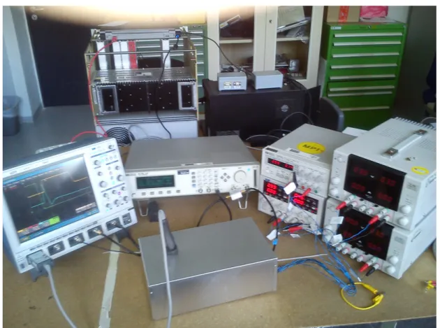
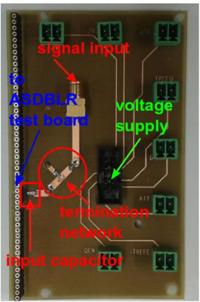
5. Electronics tests 47 5.1. The adapter board and test set-up . . . . 47
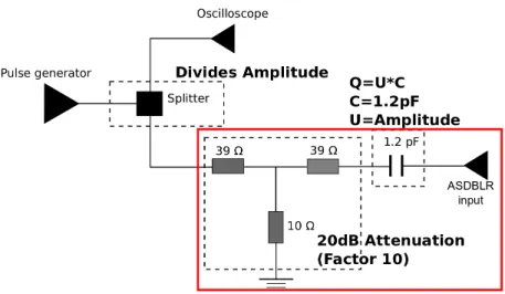
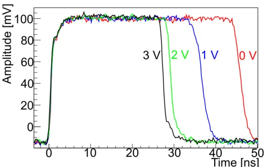
5.2. Pulse generator tests . . . . 53
5.3. ASDBLR circuit characteristics . . . . 56
5.4. The sMDT drift tube signals . . . . 57
6. Measurements with Photon Irradiation 61 6.1. The CERN Gamma Irradiation Facility . . . . 61
6.2. The test set-up . . . . 63
6.2.1. Measurement program . . . . 68
7. Data Analysis Methods 69
7.1. Drift time spectrum . . . . 69
7.2. Background counting rate . . . . 72
7.3. Drift-tube calibration . . . . 74
7.3.1. Determination of t 0 . . . . 75
7.3.2. Time slewing corrections . . . . 77
7.3.3. t0-correction using track reconstruction . . . . 80
7.4. Single-tube resolution . . . . 82
7.5. Multiple scattering and t 0 corrections . . . . 86
7.6. Single-tube efficiency . . . . 90
8. Counting Rate Effects 93 8.1. Rate dependence of the drift-tube resolution . . . . 93
8.2. Rate dependence of the drift tube 3σ-efficiency . . . . 96
8.3. High gain measurement . . . . 100
9. Summary and Outlook 103
I. Bibliography 104
1. Introduction
CERN 1 is the biggest particle physics research laboratory in the world. It was founded in 1954. Major milestones in the field of particle physics have been achieved there. In 1983, the W- and Z-bosons were discovered. The latest discovery is the Higgs boson in 2012. For this purpose, the largest accelerator ever built, the Large Hadron Collider (LHC), has been constructed. For the next step, the search for physics beyond the Standard Model, an upgrade of the LHC to higher luminosities (HL-LHC) is planned. With the upgrade of the accelerator the requirements on the detectors at the LHC increase as well. Therefore, it will be necessary to also upgrade the detectors.
ATLAS is one of the two detectors at the LHC which were designed to discover the Higgs boson. A short overview of the ATLAS experiment is given in Chap. 1.2. The Monitored Drift Tube (MDT) chambers used in the ATLAS muon spectrometer and their further development, the small-diameter Monitored Drift Tube (sMDT) chambers, are subject of this thesis. The by a factor of 2 smaller tube diameter gives the sMDT chambers an order of magnitude higher counting rate capability. The reduc- tion of the diameter improves the muon tracking efficiency and spatial resolution at high background counting rates expected at HL-LHC. To make maximum use of the new faster muon detectors, also the readout electronics has to be adapted. Fast shaping of the signal and active baseline restoration (BLR) are desirable. The test of the baseline restoration concept for the ATLAS muon chamber read- out is the topic of this thesis. After a short introduction of the ATLAS detector, the main focus is on the MDT (see Chap. 2) and sMDT (see Chap. 3) chambers. In Chap. 4, the standard MDT readout electronics is discussed and the new baseline restoration solution introduced. The test of new readout electronics in the laboratory and at high γ irradiation rates at CERN is described in Chapters 5 and 6, respectively. Finally, a summary and outlook are given in Chap. 9.
1.1. The Large Hadron Collider
The Large Hadron Collider (LHC) at CERN is the world’s most powerful accelerator. It accelerates bunches of protons in a 27 km circumference ring in opposite directions. The proton beams are brought to collisions at several points along the ring where the detectors are stationed. The proton bunch crossings are taking place at a frequency of 40 MHz, i.e. every 25 ns. The center-of-mass energy was initially 7 and 8 TeV in 2010/11 and 2012, respectively and will be increased to 13 TeV in spring 2015 after the current upgrade period [1]. For measurements with higher accuracy or for the discovery of new particles, the LHC design luminosity of 10 34 cm −2 s −1 may not be enough. Therefore, the planned LHC upgrades [2] will increase the luminosity by up to a factor of 7 compared to the design luminosity. The final stage of increasing the LHC luminosity will be reached in 2023 with the upgrade to High-Luminosity LHC (HL-LHC) [3].
1 Conseil Europ´ een pour la Recherche Nucl´ eaire
1.2. The ATLAS detector
The ATLAS experiment [4] (see Fig. 1.1) is one of the two general-purpose detectors at the Large Hadron Collider for tests of the Standard Model of particle physics and searches for new physics. The detector has a length of 46 m and a height of 25 m. It is one of the biggest particle physics detectors ever built. More than 3000 scientists from 38 countries are working in the ATLAS collaboration. It consists of several sub-detectors which are described in the following.
The Inner Tracking Detector [5] is the innermost detector closest to the beam pipe which consists of three parts, the Silicon Pixel and Silicon Strip Detectors (SCT) and the Transition Radiation Tracker (TRT). The part closest to the interaction point consists of three layers of pixel detectors followed by four layers of silicon microstrip detector providing four precise coordinate measurements along a charged particle track. The SCT measures the tracks and momenta of charged particles and the positions of the proton interaction point and of decay vertices in a 2 T solenoidal magnetic field.
The outermost part is the transition radiation tracker (TRT). It consists of straw drift tubes with a diameter of 4 mm filled with a gas mixture of Xenon (70%), CO 2 (27%) and O 2 (3%). The Inner Detector is surrounded by a superconducting solenoid coil.
Figure 1.1.: The ATLAS detector and its sub-systems [4]. The Inner Detector [5] consists of the
Pixel Detector, the SCT tracker and the TRT tracker followed by the electromagnetic and
hadronic Liquid Argon Calorimeters [6] and the hadronic Tile Calorimeter [7]. The out-
ermost system is the Muon Spectrometer [9]. A superconducting solenoid magnet is used
for the Inner Detector and superconducting toroid magnets for the Muon Spectrometer.
Chapter 1. Introduction
To measure the energies of particles, calorimeters [6] [7] surrounding the Inner Detector are used. The particles lose their energy in absorber plates producing secondary particles which are measured by the active detection medium. The Electromagnetic Calorimeter (ECAL) consists of copper absorber plates with gaps filled with liquid Argon (LAr) as active medium. Electrons and photons deposit all their energy in the ECAL, a fact which is used for their identification. The Hadronic Calorimeter (HCAL) consists of iron absorber plates and scintillating plastic tiles as active medium in the barrel part and of copper and tungsten plates in LAr in the end-caps. Hadrons are absorbed in the HCAL due to their strong interaction. The calorimeters are surrounded by the Muon Spectrometer described in the next section.
The large majority of proton-proton collisions at the LHC produces no interesting events for physics studies. A very selective trigger system [8] is used to discriminate the interesting events. It is divided into three stages. The Level-1 trigger uses the information of fast muon trigger chambers and of the calorimeters and is completely implemented in hardware. It reduces the event rate to 100 kHz with a time latency of 2.5 µs. The Level-2 trigger consists of a processor farm which analyzes in more detail the regions of interest identified by the Level-1 trigger. It reduces the Level-1 trigger rate to 3.5 kHz with a time latency of 40 ms. The last stage is the Event Filter which takes about 4 seconds of processing time per event. The offline reconstruction software processes the whole detector information. The maximum output event rate stored on disk is 200 Hz.
1.3. The ATLAS Muon Spectrometer
In the ATLAS Muon Spectrometer [4] muons are identified and reconstructed in a toroidal magnetic field. It has been designed to provide precise muon momentum measurement over a wide momentum range up to 1 TeV/c with three layers of muon detectors (see Fig. 1.2). The momentum measurement is based on magnetic deflection which is provided by a large barrel toroid and two end-cap magnets (see Fig. 1.2). The field is configured to be mostly orthogonal to the muon track such that maximum magnetic bending is achieved.
Three precise muon trajectory measurements are done in the barrel region (see Fig. 1.3, green parts) where three cylindrical detector layers are arranged around the beam axis and in the end-cap region (see Fig. 1.3, blue and yellow parts) the three layers are arranged in planes perpendicular to the beam axis.
Precise track coordinate measurements are done by Monitored Drift Tube (MDT) Chambers, which are part of this thesis and discussed in more detail in Chap. 2. They provide coordinate measurements with 80 µm resolution. Only in the very forward region close to the interaction point the MDT chambers are replaced by Cathode Strip Chambers (CSC), which are capable of higher background radiation. CSC are multi-wire proportional chambers with segmented cathodes, providing 60 µm resolution. They can handle up to 1000 Hz/cm 2 uncorrelated background rate.
In addition to muon track reconstruction the ATLAS muon spectrometer is also capable of providing information for the Level 1 trigger. Requirements in barrel and end-cap region are different such that two different detector types have been chosen. Resisitve Plate Chambers (RPC) are installed in the barrel while in the end-caps Thin Gap Chambers (TGC) are used. TGC’s are mulit-wire proportional chamber with 99% probability that signals arrive in less than 25 ns allowing bunch crossing identification. RPC’s are gaseous parallel electrode-plate detectors with two resistive plates kept parallel at a distance of 2 mm and capacitive coupling to metallic plates to read out signals.
They can provide proton bunch crossing identification as well. For more information of the ATLAS
muon spectrometer and the individual detectors see [9].
Figure 1.2.: The ATLAS muon spectrometer [4] is used for muon identification and muon track and
momentum reconstruction. It consists of four different detector types. Thin Gap Cham-
bers (TGC) and Resistive Plate Chambers (RPC) are used as trigger chambers in the
end-caps and in the barrel part, respectively. The Monitored Drift Tube (MDT) cham-
bers are used for precise track reconstruction. In the inner layer of the very forward region
CSC chambers are used as tracking detectors.
Chapter 1. Introduction
1.4. Upgrade of the LHC
The upgrade of the LHC to the HL-LHC [3] with 7 times the design luminosity of 10 34 cm −2 s −1 increases requirements on the detectors which have to cope with higher background radiation. Back- ground radiation may cause a significantly reduction of muon track finding efficiency and may lead to wrong trigger decisions. It occurs due to interaction of the proton collision products in the detector, the support structures and the shielding. The uncorrelated cavern background mainly consists of thermal neutrons and γ rays.
The ATLAS components were tested to withstand background radiation at design luminosity (with
an additional safety factor of 5). The HL-LHC will exceed this value. Due to the fact that the back-
ground rate is expected to be roughly proportional to the luminosity, an increase by about a factor 7
at HL-LHC is expected. The expected background rates in the detector are shown in Fig. 1.3.
2 4 6 8 10 12 14 16 18 20 2
4 6 8 10 12bm
0 BIL BML BOL
EEL
EML EOL
1 2 3 4 5 6
1 2 3 4 5 6
EIL4
0
1 2 3 4 5 6
1 2 3 4 5 6
1 2 3 4 5
1 2
3
End)cap magnet y
z 1
2
127 127
Expectedbcavernbbackgroundbrateb[kHzbperbtube]
66.7 76.1 77.0
26.6
23.1 81.8 91.8
46.8 78.8 13.5
9Lb=b7b·b10 34 bcm )2 bs )1 (
105
35.4 49.0 51.0
(a) Counting rate per drift tube [kHz].
2 4 6 8 1W 12 14 16 18 2W
2 4 6 8 1W 12bm
W BIL BML BOL
EEL
EML EOL
1 2 3 4 5 6
1 2 3 4 5 6
EIL4
W
1 2 3 4 5 6
1 2 3 4 5 6
1 2 3 4 5
1 2
3
End9cap magnet y
z 1
2
274 173
Expectedbcavernbbackgroundbrateb[HzbSbcm 2 ]
52 42 18 51
22 76 86
72 43
12
(Lb=b7b·b1W 34 bcm 92 bs 91 =
1W3
58 36 29
NSW
(b) Hit rates in MDT drfit tubes [Hz/cm 2 ]
Figure 1.3.: Background rates expected in the MDT chambers of the ATLAS muon spectrometer at
HL-LHC [10] at a luminosity of L = 7 · 10 34 cm −s s −1 .
2. The Monitored Drift Tube Chambers
The Monitored Drift Tube (MDT) chambers are the muon tracking detectors of the ATLAS Muon Spectrometer. They measure muon tracks with high spatial resolution. In Tab. 2.1 the operating parameters of the MDT chambers are shown. Most of the ATLAS MDT chambers consist of two multilayers of drift tubes with three or four tube layers each as shown in Fig. 2.1. The longitudinal cross section of a drift tube with the endplugs of the drift tubes holding the sense wire is displayed in Fig. 2.2. The wires are positioned in a chamber via external references on the endplugs with an accuracy of better than 20 µm.
Figure 2.1.: Schematic view of a Monitored Drift Tube (MDT) chamber [4]. The chambers used in ATLAS vary in length and width, but all consist of two multilayers of drift tubes with three or four tube layers each. An optical monitoring system using RASNIK sensors [11]
(red light paths) measures deformations caused by temperature gradients and mechanical
stress.
plastic insolator (Noryl)
crimp wire fixation precision wire-locator
O-ring seal
gas inlet aluminum ring
(external reference)
Figure 2.2.: Longitudinal cross section of a MDT tube [4]. The endplugs seal the tube, contain the gas inlet, hold the sense wire under tension, insolate it electrically against the tube wall, and position it relative to an external reference used for chamber assembly.
Table 2.1.: Parameters of the MDT drift tube chambers [4]
Parameter Value
Tube material Aluminium
Outer tube diameter 29.970 mm Tube wall thickness 0.40 mm
Wire material Gold plated W/Re (97/3)
Wire diameter 50 µm
Gas mixture Ar/CO 2 (93/7)
Gas pressure 3 bar absolute
Gas gain 2·10 4
Wire potential 3080 V
Maximum drift time ≈ 700 ns Average single-tube resolution
80 µm without irradiation,
with time slewing corrections
Wire positioning accuracy < 20 µm Chamber spatial resolution
35 µm without irradiation
(2 x 4 tube layers)
Chapter 2. The Monitored Drift Tube Chambers
2.1. The drift-tube principle
The anode wire (W/Re) is placed in the tube axis at a potential of +3080 V with respect to the tube wall leading to a gas gain of 2 · 10 4 in Ar/CO 2 (93/7) gas mixture at 3 bar pressure.
The Argon atoms are ionized by a traversing muon. Along the muon path, positively charged ions and primary ionization electrons are produced in clusters. In the electric field the ions drift to the tube wall while the electrons drift to the wire (see Fig. 2.3). A muon with about 100 GeV energy produces on average 100 primary ionization clusters per cm in the Argon gas at 3 bar corresponding to a mean free path length of 100 µm [12].
The electron drift velocity depends on the local radial electric field E(r) = λ
2π 0 r (2.1)
in the drift tube with the charge per unit length λ. The field strength increases steeply towards the wire. Amplification of the primary ionization charge takes place within a radius of 150 µm around the wire. In this region, the electrons gain enough energy between collisions to ionize more gas atoms in an avalanche process.
The signal induced on the anode wire by the amplified ionization charge is registered by the readout electronics. The time difference between a trigger signal indicating the passage of a muon through the tube and the measured arrival time of the primary ionization avalanche at the wire corresponds to the electron drift time. From the drift time, the drift distance, the distance of closest approach between the muon track and the anode wire, is determined using the calibrated space-to-drift time relation specific for the drift gas and the tube operating parameters.
Figure 2.3.: Measuring principle of a drift tube [4]. A traversing muon produces ionization clusters along its path. In the tube’s electric field, the ions drift to the tube wall while the electrons drift to the anode wire and ionize more Argon atoms in the increasing field near the wire.
Within a radius of about 150 µm around the wire an ionization avalanche occurs. The
signal induced on the anode wire is registered by the readout electronics.
2.2. The drift-tube response
A typical charge signal of an ionizing muon induced on the anode wire by the drifting electrons and ions is shown in Fig. 2.4a. The first signal component is induced by the electrons drifting to the wire and producing ionization charge in an avalanche process. Compared to the fast electrons, ions have a much lower drift velocity. Therefore, they induce a signal with very long time constant, the ’long ion tail’.
The amplifier-shaper-discriminator (ASD) chip of the MDT readout electronics amplifies and shapes the charge signal as described in Chap. 4, forming signal pulses corresponding to the electron clusters arriving successively within the maximum drift time and canceling the ion tail (see Fig. 2.4b). The ASD chip uses bipolar shaping [13] which generates an undershoot of equal area after the positive signal pulse. The arrival time of the primary electrons at the wire is determined as the time at which the first signal pulse crosses the discriminator threshold. The discriminator of the ASD chip sends a digital stop signal to the TDC 1 on the same electronics board (see Chap. 4) which measures the time interval from the start signal of the external trigger or of the LHC bunch crossing signal. The digitized time interval corresponds to the electron cluster drift time.
Time [ns]
0 200 400 600 800 1000
Current [fC/ns]
-14 -12 -10 -8 -6 -4 -2 0
(a) Raw charge signal on the anode wire.
Amplitude in arb. units
Time [ns]
0 400 800 1200 1200
(b) Bipolar shaped drift tube signal (polarity in- verted).
Figure 2.4.: MDT drift tube signals (a) before and (b) after amplification and shaping by the readout electronics. The sequential arrival of the different primary ionization clusters of the wire is visible [14].
1 Time-To-Digital Converter
Chapter 2. The Monitored Drift Tube Chambers
2.3. The drift time spectrum
In Fig. 2.5 a typical drift time spectrum of an uniformly illuminated MDT tube is shown. The number of muon tracks in each drift distance interval dN dt is in this case described by
dN dt = dN
dr dr dt = N
r max dr dt = N
r max · v drif t (t) , (2.2)
where v drif t is the drift velocity of the electrons, r max the maximum drift radius and
N =
r max
Z
0
dN
dr 0 dr 0 . (2.3)
The first part of the spectrum corresponds to short drift radii, where the electric field is strong and, therefore, the drift velocity high. Towards the end of the drift time spectrum and longer radii, the drift velocity drops.
The measured time interval is not directly the drift time but is affected also by signal propagation time delays along the drift tube and in the readout electronics leading to a time offset of the drift time spectrum. The signal propagation time is corrected for each hit using the position information along the tube from the trigger chambers. To determine the start time t 0 of the drift time spectrum after this correction, its rising edge is fitted with a Fermi function [15]
F (t) = b + A 0 1 + e −
t−t 0 T 0
. (2.4)
The inflection point of this function is defined as t 0 . The rise time of the spectrum from 10% to 90%
is given by 4T 0 , while 1/T 0 is the slope and A 0 the amplitude of the rising edge. The parameter b takes into account random hits due to noise or background radiation. t 0 has to be determined for each tube individually.
For the parametrization of the falling edge, the product of a Fermi function with an exponential is used (see Eq. 2.5).
G(t) = p 1 · e −p 2 ·t 1 + e
t−t 0 max Tmax
. (2.5)
The inflection point here is given by t 0 max while 1/T max is the slope. Although the efficiency of the drift tube drops close to the tube wall because of decreasing ionization path length, the largest measured drift times are beyond t 0 max . The maximum drift time is defined by
t max = t 0 max + 2 · T max . (2.6)
For equal operating parameters (gas composition, temperature, pressure, high-voltage, magnetic field
strength, background irradiation), t max is equal for all tubes at least within a chamber and does not
have to be determined individually. The same is true for the space-to-drift time relation (see below).
T 0 b A 0 t 0
x103
0 20 40 60 80 100 120 140
Entrie s
0 100 200 300 400 500 600 700
Drift time [ns]
700 ns
Figure 2.5.: Drift time spectrum of an uniformly illuminated MDT drift tube with a diameter of 30 mm
at nominal operating conditions [16]. The fit parameters of the rising and falling edges of
the spectrum are described in the text. The maximum drift time is about 700 ns.
Chapter 2. The Monitored Drift Tube Chambers
2.4. The space-to-drift time relation
The muon track reconstruction uses the information about the measured minimum distances between the muon path and the anode wires which are determined from the measured drift times in the tubes via the space-to-drift time relation. The following methods are used to determine the space-to-drift time relation [17].
The integration method assumes homogeneous illumination of the tube by muons such that Eq. 2.2 applies. The space-to-drift time relation r(t) is determined by integrating the drift time spectrum dN/dt from t 0 to t max :
r(t) = Z t max
t 0
dr
dt 0 dt 0 = r max
N
Z t max
t 0
dN
dt 0 dt 0 . (2.7)
The result is used as a first estimate and is improved by the auto-calibration method [18] [19].
This method simultaneously minimizes the deviations of the means of the distributions of the track residuals
∆(t) = r(t) − d (2.8)
from zero in several layers of a chamber as a function of the drift time, starting from the space-to-drift time relation of the integration method. The shortest distance d of the reconstructed straight track y = m · z + b described by slope m and y-axis intercept b, to the wire (see Fig. 2.7) is given by
d = | b + mz tube − y tube |
√ 1 + m 2 . (2.9)
The auto-calibration algorithm iteratively corrects the r(t) relationship in all tubes hit by the track in intervals of t,
r i+1 (t) = r i (t) − h∆(t)i , (2.10)
where h∆(t)i is the mean of the residual distribution in the time interval. This procedure takes into
account the correlations between the hits on a track and between different tracks minimizing the
number of tracks required to achieve the desired precision of the calibration. In Fig. 2.6, the typical
space-to-drift time relation of a 30 mm diameter MDT drift tube at nominal operating conditions is
shown. The r(t) relation is non-linear reflecting the dependence of the drift velocity on the electric
field and, therefore, on the drift radius which is a property of the Ar/CO 2 drift gas.
0 2 4 6 8 10 12 14 0
100 200 300 400 500 600 700
Drift radius (r) [mm]
Drift time ( t) [ns]
Figure 2.6.: Space-to-drift time relation of a 30 mm diameter MDT drift tube at nominal operating
conditions [16]. The non-linearity reflects the dependance of the drift velocity on the
electric field and, therefore, on the drift distance r.
Chapter 2. The Monitored Drift Tube Chambers
y
Z
Figure 2.7.: Principle of track reconstruction in a MDT chamber [16]. The drift tubes are arranged in
multilayers with 3 or 4 tube layers each. The drift distances measured by the drift tubes
illustrated as green circles, are used for the track reconstruction. The algorithm minimizes
the sum of the squared track residuals weighted by the squared drift tube spatial resolution
as a function of the drift distance (see Eq. 2.12).
2.5. Track reconstruction
In the end a reconstructed muon track with high precision is produced. To reconstruct a muon track the measured drift times are used [20]. As a MDT chamber consists of 6 (8) layers, up to 6 (8) drift radii are measured along the muon path (see Fig. 2.7). Neglecting bending in the magnetic field within a chamber, the muon tracks are straight and can be parametrized as
y = mz + b (2.11)
in the chamber coordinate system (see Fig. 2.7) where the y and z axes are perpendicular to the tube axis (x) and y (z) is perpendicular (parallel) to the chamber plane. A χ 2 -fit of this function to the measured distances is performed with
χ 2 =
N hits
X
i=1
(r(t i ) − d i ) 2
σ 2 i , (2.12)
where r(t i ) is the radius of the drift circle of the i th hit along the track and σ i = σ(d i ) the drift tube resolution at the distance-of-closest-approach d i of the fitted track to the wire. d i is calculated using Eq. 2.9 and 2.11.
2.6. Single-tube resolution
The spatial resolution σ of tube i is determined from the distribution of the residuals of the measured drift radii r i with respect to the distance d i of the reconstructed track to the wire with correction for the extrapolated track error [21]:
σ 2 (d i ) = V ar(r i − d i ) + σ f it 2 (d i ) . (2.13) The drift tube resolution is affected by several parameters (see for example [21]), in particular by the signal amplitude and the discriminator threshold. The signal amplitude is determined by the collected ionization charge and affects the accuracy of the time measurement (see Fig. 2.8) and, therefore, the single-tube resolution [22]. Signals with higher amplitude also have a steeper rising edge such that the signal crosses the threshold earlier and with less jitter than signals with lower amplitude. This time-slewing effect and its correction is discussed in Chap. 7.3.2. In Fig. 2.8 signals with different amplitudes and the corresponding shifts in the threshold crossing time are illustrated. In addition to the drift time, the readout electronics also measures the deposited charge (proportional to the signal amplitude) allowing for time-slewing corrections.
In Fig. 2.9 the spatial resolution of a MDT drift tube as a function of the drift radius at nominal
operating conditions is shown. The single-tube resolution without background irradiation is on average
(98 ± 2)µm. With time-slewing corrections it can be improved to (84 ± 2)µm [16] [23].
Chapter 2. The Monitored Drift Tube Chambers
Time (ns) Threshold
25 50 75
0.2 0.4 0.6 0.8 1
100 Signal charge [arb. units]
Figure 2.8.: The discriminator threshold crossing time depends on the amplitude of the signal. Varia-
tions in the amplitude leading to an uncertainty in the threshold crossing time measure-
ment [24]. The MDT readout electronics (see Chap. 4) measures and digitizes, in addition
to the threshold crossing time, the charge in the rising edge of the signal pulse with an
ADC which is a measure of the signal amplitude. The ADC measurement can be used
to correct the time measurement, so-called time-slewing-corrections (see Chap. 7.3.2), the
typical signal width of an individual ionization pulses of 100 ns measured by the MDT
readout electronics is also indicated.
Figure 2.9.: Spatial resolution of MDT drift tubes as a function of the drift radius r at nominal operat-
ing conditions without background irradiation with and without time-slewing corrections
(TSC). Without TSC, the average single-tube resolution is (98 ± 2) µm. While TSC
improves it to (84 ± 2) µm [16] [23].
Chapter 2. The Monitored Drift Tube Chambers
2.7. Single-tube efficiency
Muons generate enough charge to produce signals which exceed the threshold and, therefore, the muon detection efficiency of an MDT drift tube is 100%, expect for muon tracks close to the tube wall. When a muon passes the tube near the wall, the path length becomes short and only little primary ionization charge is produced. When the path becomes shorter than the mean free path length of the muon, it is even possible that no charge cluster arises at all.
For muon track reconstruction only hits with drift distance r hit within three times the local drift tube resolution σ of the extrapolated track distance to the wire d track , i.e. with
| r hit − d track |< 3σ(d track ), (2.14)
are used. A single-tube tracking efficiency, the so-called 3σ-efficiency, is defined as the probability to find a hit with drift radius within 3 times the local drift tube resolution of the distance of the extrapolated muon track to the wire:
3σ-efficiency = Number of events with a hit in the tube within 3σ(d track ) of the extrapolated track
Number of tracks passing the tube .
(2.15) The 3σ-efficiency of MDT drift tubes without background radiation at nominal operating conditions is shown in Fig. 2.10 for two different deadtime settings of the readout electronics.
δ-electrons knocked out of the tube walls by the penetrating muons decrease the 3σ-efficiency over the whole tube radius but more pronounced for muon tracks closer to the tube wall [19]. The ionization path of the δ-electrons frequently is closer to the wire than the original muon track leading to masking of the muon hit (see Fig. 2.11), an effect which is increasing with the distance of the muon track to the wire. The δ-electron occupies the readout electronics and the muon signal cannot be detected during the electronics deadtime.
The deadtime of the MDT readout electronics can be adjusted between the minimum of 220 ns and 820 ns, slightly longer than the maximum drift time of the MDT tubes. A signal above the discriminator threshold triggers the deadtime during which the tube is not sensitive to further hits.
When a δ-electron or background particle triggers the deadtime, subsequent muon hits within a time interval shorter than the deadtime are lost. This effect is called masking of hits. In Fig. 2.10 an increase of the 3σ-efficiency for the shorter deadtime is visible.
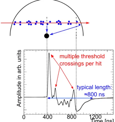
The ionization clusters of a particle traversing the tube arrive at the wire after different time intervals
causing multiple signal pulses. For short enough deadtime, it is, therefore, possible that for the same
moun or background hit the discriminator threshold is crossed more than once (see Fig. 2.12). This
increases the amount of data and triggers the deadtime again potentially leading to an larger effective
deadtime than the nominal one. To limit the amount of data and stay below the counting rate limit
per channel of 500 kHz, the deadtime of the ATLAS MDT front-end electronics is adjusted to the
maximum of 820 ns = 700 ns + 120 ns, which is larger than the maximum drift time by the typical
individual pulse length of the MDT readout electronics of about 100 ns.
0.70 0.75 0.80 0.85 0.90 0.95 1.00
0 1 2 3 4 5 6 7 8 9 10 11 12 13 14 15 asdf
3 σ -ef
ficiency
Drift radius (r) [mm]
MDT 3σ-efficiency 820 ns deadtime MDT 3σ-efficiency 220 ns deadtime
Figure 2.10.: 3σ-efficiency of a MDT drift tube as a function of the drift distance without background
irradiation at nominal operating conditions for 820 ns (max.) and 220 ns (min.) ad-
justable electronics deadtime [16]. The efficiency drop at large drift radii occurs because
the influence of δ-electrons increases with the drift radius (see text). The shorter dead-
time allows for the registration of secondary hits after 220 ns after a background hit. If
the time between the δ-electron signal and the muon signal is larger than 220 ns, the
muon is still detected recovering 3σ-efficiency with increasing drift distance.
Chapter 2. The Monitored Drift Tube Chambers
Figure 2.11.: Illustration of the masking of a muon hit by a δ-electron knocked out of the tube wall by the muon [16]. When the electron passes closer to the wire than the muon, r δe < r µ , the muon hit is not detected within a time interval after the δ-electron hit shorter than the electronics deadtime.
Amplitude in arb. units
Time [ns]
0 400 800 1200 1200
typical length:
≈800 ns multiple threshold crossings per hit
Figure 2.12.: Illustration of an ionization signal processed by the readout electronics of an MDT tube
with multiple threshold crossings. If the deadtime is short enough, secondary threshold
crossings are detected as hits triggering the deadtime again and increasing the effective
deadtime and the amount of data.
2.8. Effects of high background irradiation rates
In the presence of background irradiation, the spatial resolution is degraded due to two effects [25] [26].
The background hits produce ion space charge in the tube, which affects the drift time and gas amplification.
The ion space charge lowers the effective potential of the anode, thus lowering the gas gain, which results in a loss of signal charge and amplitude. In Fig. 2.8 pulses with different amplitudes are shown.
The pulses with highest amplitude provide the most precise time measurement. Since the drift distance measurement depends on the time measurement, the gain drop effect leads to a degradation of the spatial resolution. As the amplification takes place close to the wire, this effect is the dominating one at smaller drift radii. Measurements of the single-tube resolution as a function of the drift radius are shown for different background irradiation rates in Fig. 2.13. The degradation effect due to the gain drop close to the wire is clearly visible in the region.
The resolution degradation in the presence of background radiation at larger drift radii r & 7mm is caused by ion space charge fluctuations. The background hits occur randomly leading to stochastic fluctuations of the ion space charge and, therefore, of the electric field in the tube which cannot be resolved by the space-to-drift time calibration. For a non-linear drift gas like Ar/CO 2 (93/7) in particular, this results in fluctuations of the drift velocity affecting the drift time measurement and leading to a degradation of the single-tube resolution. This effect increases rapidly for drift radii larger than 7 mm and dominates at large drift radii (see Fig. 2.13).
Not only the single-tube resolution is affected by background radiation but also the single-tube muon efficiency [25]. Every background hit triggers the deadtime, and may mask a hit of a traversing muon.
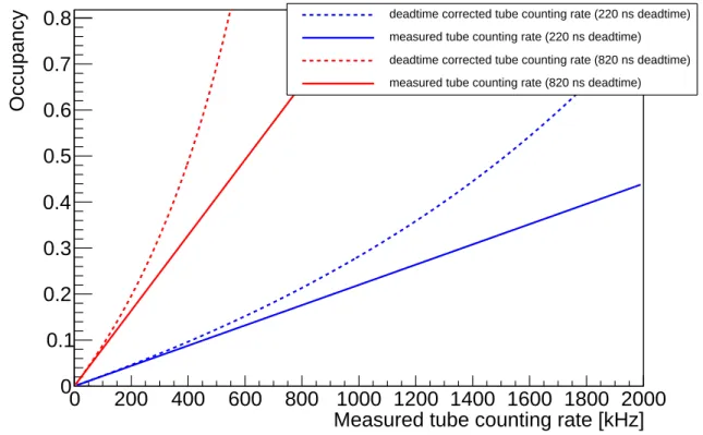
The efficiency drop increases with the hit rate. The occupancy of a drift tube (see Fig. 2.14) defined by
occupancy = measured tube counting rate [Hz] · deadtime [s] (2.16) is a measure of the masking effect and determines the 3σ single-tube efficiency as a function of the rate. The MDT drift tube 3σ-efficiency as a function of the drift radius is shown in Fig. 2.15 for different background rates and maximum (820 ns) and minimum (220 ns) deadtime. Degradation with increasing background rate is visible for both deadtime settings but less for the short deadtime.
In Fig. 2.14 the occupancy as a function of the measured counting rate is shown for the maximum (820 ns) and minimum (220 ns) deadtime. The corrected rate takes into account that background particles are masked if they occur during the deadtime as well as the muons. It can be determined with following equation
corrected tube counting rate[Hz] = measured tube counting rate [Hz]
1 − (measured tube counting rate [Hz] · deadtime [s]) . (2.17)
The influence of the deadtime is obvious.
Chapter 2. The Monitored Drift Tube Chambers
Drift radius (r) [mm]
0 2 4 6 8 10 12 14
Single-tube-resolution [mm]
0 0.05 0.1 0.15
0.2 0.25
coord
Entries 0
Mean x 0
Mean y 0
RMS x 0
RMS y 0
coord
Entries 0
Mean x 0
Mean y 0
RMS x 0
RMS y 0
No irradation 155 Hz/cm 2
259 Hz/cm 2
523 Hz/cm 2
818 Hz/cm 2
Gain drop Space charge fluct uation s
Figure 2.13.: Spatial resolution of MDT drift tubes as a function of the drift radius at nominal op-
erating conditions for different background rates [27]. The ion space charge in the tube
lowers the electric field near the anode wire causing a drop of the gas gain and degrada-
tion of the single-tube resolution particularly at small drift radii. For large drift radii,
the fluctuations of the space charge in time gain influence altering the electric field and
the drift velocity and deteriorating the time measurement and spatial resolution.
Measured tube counting rate [kHz]
0 200 400 600 800 1000 1200 1400 1600 1800 2000
Occupancy
0 0.1 0.2 0.3 0.4 0.5 0.6 0.7
0.8 deadtime corrected tube counting rate (220 ns deadtime)
measured tube counting rate (220 ns deadtime) deadtime corrected tube counting rate (820 ns deadtime) measured tube counting rate (820 ns deadtime)
Figure 2.14.: The occupancy as a function of the measured tube counting rate for maximum (820 ns) and minimum (220 ns) deadtime.
r [mm]
0 2 4 6 8 10 12 14
efficiency σ 3
0 0.2 0.4 0.6 0.8 1
No irradiation Attenuation factor 10 Attenuation factor 5
(a) 3σ-efficiency for maximum deadtime [14].
r [mm]
0 2 4 6 8 10 12 14
efficiency σ 3
0 0.2 0.4 0.6 0.8 1
No irradiation Attenuation factor 10 Attenuation factor 5
(b) 3σ-efficiency for minimum deadtime [14].
Figure 2.15.: 3σ-efficiency of MDT drift tubes as function of the drift radius r for maximum and min- imum front-end electronics deadtime. The attenuation factors corresponds to different background rates leading to degradation of the 3σ-efficiency at high background rates.
Efficiency gain due to a shorter deadtime is visible.
Chapter 2. The Monitored Drift Tube Chambers
2.9. The MDT readout electronics
In order to supply the drift tubes with high voltage (HV), provide an external trigger, set the pro- grammable electronics parameters, process the analog charge signal and store the digitized output data, the tubes are connected to electronics boards.
For high voltage supply between anode wires and tube walls and to connect them to the readout electronics in groups of 24, two different types of printed circuit boards, the so-called high-voltage (HV) and readout (RO) hedgehog cards, are used. To protect the readout electronics against shorts, a 1 MΩ resistor for each channel is mounted on the hedgehog cards at the HV supply end of the tubes.
In addition, a high frequency filter protects against pick-up noise from the high voltage cables (see Fig. 2.16, right hand side). On the read-out end of the tubes, the hedgehog cards couple the wire capacitively to the front-end electronics (see Fig. 2.16, left) [28].
The mezzanine cards are mounted directly via a connector on the signal hedgehog cards with a grounded shielding plate in between to minimize noise pick-up. The tube current signals are amplified and shaped by the ASD chip. Each mezzanine card carries three ASD chips with 8 readout channels each. The different ASD stages are described in Chap. 4. If the signal exceeds the discriminator threshold, a digital signal is sent to a TDC on the mezzanine card. The TDC time measurement is started by an external trigger (the TTC 2 signal in ATLAS or from a dedicated trigger system for cosmic muons, for instance) and stopped when the digital signal from the ASD arrives indicating the threshold crossing time.
To measure the MDT signal pulse amplitude, a Wilkinson-ADC is integrated on the ASD chip. As mentioned earlier, the measured drift time is affected by the signal pulse height. The ADC measure- ment [28] can be used to correct the time measurement (time slewing corrections).
The MDT readout system is illustrated in Fig. 2.17. The readout electronics is connect to the LHC TTC system providing the bunch crossing time, to the data acquisition system via the MDT Readout Driver (MROD) and to the detector control system (DCS) via a CAN bus interface in the ELMB 3 . The Chamber Service Module (CSM) [40] distributes the electronics parameter settings and the trig- ger signal to the individual mezzanine cards and collects the data from them to send them via an optical link and the readout driver (MROD) to the data acquisition (DAQ) system. One CSM can handle up to 18 mezzanine cards. The trigger signal is sent via an optical link to the CSM. The electronics parameter settings are transmitted using the JTAG 4 protocol, via the CAN 5 bus, and the ELMB module for the detector control system (DCS) reading temperature and magnetic field on the chambers.
2 Timing, Trigger and Control
3 Embedded Local Monitoring Board
4 Joint Test Action Group
5 Controller Area Network
10n
Figure 2.16.: Schematics of a MDT tube with readout electronics (left end) and high voltage con- nection (right end) [28]. On the HV hedgehog cards, a 1 MΩ resistor is mounted to protect the electronics against short circuits between tube wall and wire (see text). The signal hedgehog cards couple capacitively the tube to active readout electronics on the mezzanine cards (see text).
Tubes
Hedgehog Mezzanine
80Mb/s
TTCrx 200 Mbyte/s MROD
Gigabit TTC Fibre TTC
Clk, L1A, Calib
Mux
Monitor JTAG
ELMB Mux 18 Mezzanine
Cards Maximum
64 ADCs ELMB
CAN Bus
ROS To TTCvi Central Control
CSM
Opto-isolated JTAG Serial to Parallel
Xtmr
Ethernet
ASD ASD ASD
AMT
3 Octal ASD 24 Chan/TDC
Power Passive Interconnect
Figure 2.17.: Schematics of the MDT chamber readout chain [28]. The tubes are connected to so-
called hedgehog cards for high-voltage and signal distribution to opposite ends of groups
of 24 tubes. The active read out boards (mezzanine cards) are mounted directly on the
hedgehog boards. The three ASD chips mounted on one mezzanine card take care of 24
tubes. The mezzanine cards are connected to a Camber Service Module (CSM) which can
handle up to 18 cards. The CSM distributes the trigger signals (TTC) to the individual
mezzanine cards and collects the drift time and charge measurements from them and
sends them via the MDT Readout Driver (MROD) to the data acquisition system. The
JTAG protocol transmitted via the CAN bus is used to set the programmable electronics
parameters.
3. The Small-Diameter Monitored Drift Tube Chambers
In the course of the luminosity upgrades of the LHC, the background radiation rates in the ATLAS muon spectrometer (see Chap. 1.3) will increase and the MDT chambers will reach the limits of their rate capability. The so-called small-diameter Monitored Drift Tube (sMDT) chambers have been developed to cope with the up to ten times higher background rates (see Chap. 1.4). The diameter of the drift tubes is reduced by a factor of 2. The operating parameters (see Tab. 3.1) have been chosen to match with the existing ATLAS gas distribution system. The same small gas gain as for the MDT chambers is used to prevent aging of the drift tubes. This is realized by reducing the applied voltage to 2730 V [29]. The same readout electronics as for the MDT chambers can be used. Optimization of the front-end electronics for the sMDT readout is studied in this thesis. In the following sections, single-tube-resolution and efficiency of the sMDT tubes at high background rates and their advantages compared to the MDT chambers are discussed.
3.1. Advantages of the sMDT chambers
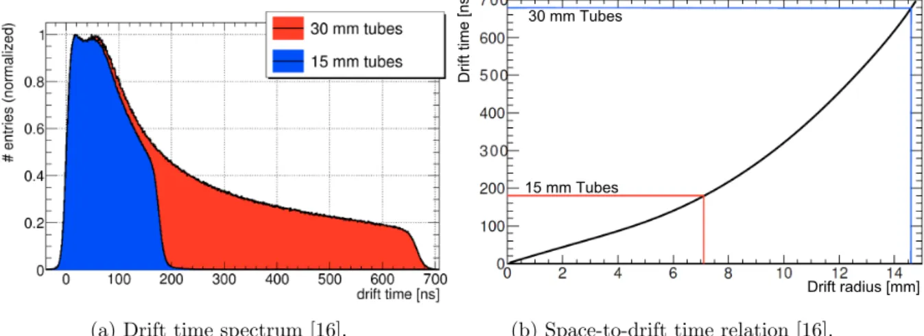
All deteriorating effects of high irradiation discussed above (see Chap. 2.8) are reduced by the diameter reduction [25] [26] [30]. In Fig. 3.1a, a sMDT drift time spectrum at nominal operating parameters is shown in comparison with a MDT drift time spectrum. The rising edge stays the same as for MDT drift tubes, but the maximum drift time and the slow slope region respectively are reduced, leading to an almost linear space-to-drift time relation (see Fig. 3.1b). The maximum electron drift time is reduced from about 700 ns to 185 ns. The tube diameter reduction also eliminates multiple threshold crossings, therefore the front-end electronics deadtime can be reduced to the minimum 220 ns without increasing the amount of data per tube.
The masking effect depends directly on the occupancy of a drift tube defined in Eq. 2.16. Since it is proportional to the deadtime it decreases by a factor of 3.7 = 820 220 ns ns from the maximum (MDT) to the minimum (sMDT) deadtime. Due to the fact that the cross section per unit length of the sMDT tubes exposed to uniform irradiation is only half as large as the one of the MDT tubes, the hit rate in the sMDT tubes decreases by another factor of 2. The occupancy therefore reduces in total by a factor of 7.4 = 2 · 3.7 decreasing the masking effect.
The gain drop in MDT and sMDT tubes due to background radiation can be calculated using the Diethorn formula [31]
G(U, ρ) = U
A(ρ) B U
, (3.1)
where ρ is the gas density and U the anode potential. A(ρ) and B are defined as A(ρ) = r w ln
r t r w
E min
ρ ρ 0
, B = ln( r r t
w )∆V
ln 2 , (3.2)
Table 3.1.: Operating parameter of the sMDT drift tubes [16] [29]
Parameter Value
Tube material Aluminium
Outer tube diameter 15.000 mm
Tube wall thickness 0.40 mm
Wire material Gold plated W/Re (97/3)
Wire diameter 50 µm
Gas mixture Ar/CO 2 (93/7)
Gas pressure 3 bar absolute
Gas gain 2 · 10 4
Wire potential 2730 V
Maximum drift time 185 ns
Average single-tube resolution
104 µm without irradiation,
with time slewing corrections
Wire positioning accuracy / chamber < 20 µm
Chamber resolution 35 µm
with the normal gas density ρ 0 , the wire radius r w and the inner tube radius r t . The gas parameters
∆V and E min are the minimum ionization potential and the minimum field strength necessary for the electrons to reach the ionization energy, respectively. In Fig. 3.2, the gas gain G relative to the nominal gas gain G 0 = 2 · 10 4 is shown as a function of the background rate. In contrast to the masking effect depending on the tube counting rate, the gain drop and space charge fluctuation effects are local space charge effects, therefore, independent of the tube length. The potential drop near the wire corresponding to the gain drop is in first approximation given by
∆U = r t 3 qΦ ln r r t
w
4π 0 µV 0 , (3.3)
where q is the total avalanche signal charge per particle crossing and Φ the particle flux per unit
detector area [24]. It is proportional to r t 3 for photons and neutrons converting in the tube wall and
producing secondary charged particles which ionize the gas close to the tube wall. The wire potential
drop in sMDT compared to MDT tubes is therefore reduced by a factor of 8.7 = (14.6 (7.1 mm) mm) 3 3 in the
first approximation. Charged particles ionize directly the gas traversing the whole tube diameter such
that the voltage drop is proportional to r t 4 because the ionization charge is proportional to r t .
The effect of space charge fluctuations is almost completely eliminated in sMDT tubes. As mentioned
before, the space-to-drift time relation for sMDT tubes is almost linear (see Fig. 3.1b) and the electron
drift velocity, therefore, largely independent of the local electric field. The expected improvement in
the drift tube spatial resolution by eliminating the effect of space charge fluctuations by reducing the
tube diameter by a factor of 2 can be evaluated from Fig. 2.13.
Chapter 3. The Small-Diameter Monitored Drift Tube Chambers
(a) Drift time spectrum [16].
Drift radius [mm]
Drift time [ns]
30 mm Tubes
15 mm Tubes
(b) Space-to-drift time relation [16].
Figure 3.1.: Drift time spectrum and space-to-drift time relation of sMDT and MDT drift tubes.
The region of the drift time spectrum with small slope is eliminated leading to an almost
linear space-to-drift time relation which makes the drift tubes less sensitive of space charge
fluctuations. The maximum electron drift time is reduced by a factor of 3.8 from 700 ns to
185 ns and multiple threshold crossings are eliminated even for the minimum electronics
deadtime of 220 ns which therefore is preferred of the sMDT tubes to achieve maximum
efficiency.
2 ] background flux [kHz/cm γ
10 -1 1 10 10 2
0 Relative gas gain G/G
0 0.2 0.4 0.6 0.8 1
∅ MDT 30 mm
sMDT
∅ 15 mm
Figure 3.2.: Gas gain relative to the nominal gas gain G 0 as a function of the γ flux registered by the
tube of sMDT and MDT drift tubes as given by the Diethorn formula [14]. With increasing
background rates and space charge density the gas gain decreases but significantly less for
the sMDT tubes. Since the space charge depends on the effective wire potential, the gas
gain according to the Diethorn formula has to be calculated iteratively.
Chapter 3. The Small-Diameter Monitored Drift Tube Chambers
3.2. Single-tube resolution and efficiency
In Fig. 3.3 the single-tube resolution as a function of the γ background rate is shown for MDT and sMDT tubes. The average sMDT single-tube resolution without irradiation of (106 ± 2) µm [16] is worse than the one of the MDT tubes of (84 ± 2) µm (including time slewing corrections) because the resolution improves with the drift distance. With increasing background rate, however, the spatial resolution of the sMDT tubes deteriorates much less than for MDT tubes. In the sMDT case, measurements for two different deadtimes, 220 ns and 600 ns, are shown. In the first case, the deterioration of the resolution is worse because of signal pile-up [23] effects. The study of these effects is subject of this thesis and discussed in the next section.
The 3σ-efficiency in the non-irradiated case is similar for MDT and sMDT tubes, only about 94%
because of δ-electron emission. For sMDT tubes, however, the 3σ-efficiency deteriorates much less with increasing counting rate than for MDT tubes (see Fig. 3.4). The masking effect is modeled by the relation
3σ-efficiency = 0.94
1 + corrected background rate [Hz] · deadtime [s] (3.4) depending on the deadtime. The measurements for MDT tubes with maximum deadtime resulting of nominal 820 ns fit the prediction with a deadtime of 827 ns. The measurements for sMDT tubes with minimum deadtime setting of nominal 220 ns correspond to a fitted deadtime parameter of 338 ns.
The 3σ-efficiency prediction for sMDT tubes for nominal adjusted deadtime of 220 ns is significantly
better. The degradation in the measurements is again due to signal pile-up effects [23] discussed in
the next Section.
background rate [kHz]
0 200 400 600 800 1000 1200 1400 1600 γ
Single-tube-resolution [mm]
0.04 0.06 0.08 0.1 0.12 0.14 0.16 0.18 0.2 0.22
MDT (820 ns deadtime) sMDT (220 ns deadtime) sMDT (600 ns deadtime)
degradiation due to signal pile-up
smdt Entries 47 Mean 4271 Mean y 0.1248 RMS 3374 RMS y 0.01202
2 ] background rate [Hz/cm
0 2000 4000 6000 γ 8000 10000
Single-tube-resolution [mm]
0.04 0.06 0.08 0.1 0.12 0.14 0.16 0.18 0.2 0.22
smdt Entries 47 Mean 4271 Mean y 0.1248 RMS 3374 RMS y 0.01202
![Figure 1.3.: Background rates expected in the MDT chambers of the ATLAS muon spectrometer at HL-LHC [10] at a luminosity of L = 7 · 10 34 cm −s s −1 .](https://thumb-eu.123doks.com/thumbv2/1library_info/4017404.1541512/10.892.116.792.131.1036/figure-background-rates-expected-chambers-atlas-spectrometer-luminosity.webp)
![Figure 4.1.: The analog circuits scheme of the ASD chip for the MDT readout electronics (see text) [13]](https://thumb-eu.123doks.com/thumbv2/1library_info/4017404.1541512/40.892.136.760.227.480/figure-analog-circuits-scheme-asd-chip-readout-electronics.webp)
![Figure 4.4.: Schematics of the simulation done with ADS [34]. The circuit is equal to the one in Fig](https://thumb-eu.123doks.com/thumbv2/1library_info/4017404.1541512/43.892.207.676.476.758/figure-schematics-simulation-ads-circuit-equal-fig.webp)