Investigating the effect of El Niño on nitrous oxide distribution in the eastern tropical South Pacific

(1)

https://doi.org/10.5194/bg-16-2079-2019

Investigating the effect of El Niño on nitrous oxide distribution in the eastern tropical South Pacific

Qixing Ji¹, Mark A. Altabet², Hermann W. Bange¹, Michelle I. Graco³, Xiao Ma¹, Damian L. Arévalo-Martínez¹, and Damian S. Grundle^1,4

1GEOMAR Helmholtz Centre of Ocean Research Kiel, Kiel, 24105, Germany

2School for Marine Science & Technology, University of Massachusetts Dartmouth, New Bedford, Massachusetts, USA

3Dirección General de Investigaciones Oceanográficas y cambio Climático, Instituto del Mar del Perú (IMARPE), P.O. Box 22, Callao, Perú

4Bermuda Institute of Ocean Sciences, St. George’s, GE01, Bermuda Correspondence:Qixing Ji (qji@geomar.de)

Received: 19 October 2018 – Discussion started: 6 November 2018 Revised: 29 April 2019 – Accepted: 2 May 2019 – Published: 17 May 2019

Abstract.The open ocean is a major source of nitrous oxide (N₂O), an atmospheric trace gas attributable to global warming and ozone depletion. Intense sea-to-air N₂O fluxes occur in major oceanic upwelling regions such as the eastern tropical South Pacific (ETSP). The ETSP is influenced by the El Niño–Southern Oscillation that leads to inter-annual varia- tions in physical, chemical, and biological properties in the water column. In October 2015, a strong El Niño event was developing in the ETSP; we conduct field observations to investigate (1) the N₂O production pathways and associated biogeochemical properties and (2) the effects of El Niño on water column N₂O distributions and fluxes using data from previous non-El Niño years. Analysis of N₂O natural abundance isotopomers suggested that nitrification and partial denitrification (nitrate and nitrite reduction to N₂O) were occurring in the near-surface waters; indicating that both pathways contributed to N₂O effluxes. Higher-than-normal sea surface temperatures were associated with a deepening of the oxycline and the oxygen minimum layer. Within the shelf region, surface N2O supersaturation was nearly an order of magnitude lower than that of non-El Niño years. Therefore, a significant reduction of N2O efflux (75 %–95 %) in the ETSP occurred during the 2015 El Niño. At both offshore and coastal stations, the N₂O concentration profiles during El Niño showed moderate N₂O concentration gradients, and the peak N₂O concentrations occurred at deeper depths during El Niño years; this was likely the result of suppressed upwelling retaining N₂O in subsurface waters. At multiple

stations, water-column inventories of N₂O within the top 1000 m were up to 160 % higher than those measured in non- El Niño years, indicating that subsurface N₂O during El Niño could be a reservoir for intense N₂O effluxes when normal upwelling is resumed after El Niño.

1 Introduction

The El Niño–Southern Oscillation (ENSO) is a naturally occurring decadal climate cycle that affects the oceanic and atmospheric conditions across the equatorial Pacific (Philan- der, 1983). A pronounced effect of ENSO in the ocean is the redistribution of heat flux across the tropical and subtropical Pacific. Generally, the ENSO cycle can be divided into three phases, El Niño, La Niña, and neutral. During El Niño/La Niña years, higher/lower sea surface temperature and deepening/shoaling of the thermocline depth occur in the eastern tropical South Pacific (ETSP) (Barber and Chavez, 1983).

During El Niño years, upwelling is suppressed in the ETSP, and thus reduces upward nutrient fluxes to the surface waters causing decreased primary production (Chavez et al., 2003;

Ñiquen and Bouchon, 2004; Graco et al., 2017).

The ETSP is an oceanic region with intense sea-to-air flux of nitrous oxide (N₂O), a strong greenhouse gas and a potent ozone-depleting agent in the 21st century (Ravishankara et al., 2009). Diverse microbial processes involved in the production and consumption of N₂O occur in the ETSP, a major

(2)

oceanic oxygen minimum zone (OMZ) having a wide range of O₂concentrations spanning the sub-nanomolar level at intermediate depths (Revsbech et al., 2009) to atmospheric saturation at the surface. In the presence of oxygen, N₂O is a by-product during the first step of nitrification, i.e., ammo- nium (NH⁺₄) oxidation to nitrite (NO⁻₂) (Anderson, 1964).

Under suboxic and anoxic conditions, N₂O is produced via partial denitrification, i.e., NO⁻₂ reduction and nitrate (NO⁻₃) reduction (Codispoti and Christensen, 1985). Partial denitrification can be mediated by denitrifying bacteria using NO⁻₂ and NO⁻₃ as substrates, as well as nitrifying bacteria using only NO⁻₂, a process termed nitrifier–denitrification (Frame and Casciotti, 2010; Trimmer et al., 2016). The dominant biological sink of N2O in the ocean is the last step of denitrification where N2O is reduced to N2 under anoxic conditions (Codispoti and Christensen, 1985). Recent investiga- tions suggest that N₂O uptake by diazotrophs is another possible N₂O sink occurring at the surface waters (Farías et al., 2013; Cornejo et al., 2015). Its environmental significance awaits further exploration.

Research on the impact of ENSO on N₂O dynamics was initiated by the observation of significant reduction in oceanic N₂O effluxes during El Niño events (Cline et al., 1987; Butler et al., 1989). Recent model simulations demonstrated that ENSO events could induce lower denitrification rates, higher nitrification rates, and lower N₂O fluxes (Mogollón and Calil, 2017; Yang et al., 2017), which could be related to changes in O2and organic matter availabilities that are critical environmental factors regulating N2O production (Elkins et al., 1978; Farías et al., 2009; Arévalo- Martínez et al., 2015; Kock et al., 2016). Here we report water column hydrography, nitrogen biogeochemistry, and N₂O distribution during October 2015 when a strong El Niño event (recurrence interval >10 years) was developing (Stramma et al., 2016; Santoso et al., 2017). The natural abundance isotopomers of N₂O, i.e., the intramolecular con- figuration of stable isotopes (¹⁵N vs.¹⁴N and¹⁸O vs.¹⁶O), were used to determine the pathways of N₂O production and consumption by a simple mass balance model outlined previously (Yamagishi et al., 2007; Grundle et al., 2017). Finally, the effects of a strong El Niño event on the surface and water column N2O distributions were investigated by incorpo- rating archived ETSP datasets that demonstrated contrasting hydrography and biogeochemistry between El Niño and non- El Niño years.

2 Materials and methods

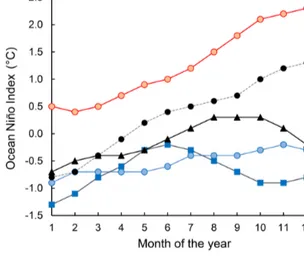
2.1 Field sampling and laboratory measurements The progress and the strength of El Niño was quantified by the Ocean Niño Index (ONI, Fig. 1), defined as the running 3- month average sea surface temperature anomaly for the Niño 3.4 region in the east-central tropical Pacific (5^◦S–5^◦N,

Figure 1.Ocean Niño Index of the years 1985 (weak La Niña), 2009 (neutral), 2011 (weak La Niña), 2012 (neutral), and 2015 (strong El Niño). Data were downloaded from http://origin.cpc.ncep.noaa.

gov/products/analysis_monitoring/ensostuff/ONI_v5.php (last access: 15 October 2018).

120–170^◦W). The 2015–2016 El Niño was a “strong El Niño event” indicated by ONI≥0.5^◦C from November 2014 to May 2016. This study was conducted on the ASTRA-OMZ SO243 cruise on board the R/VSonnebetween 5 and 22 Oc- tober 2015 from Guayaquil, Ecuador, to Antofagasta, Chile (Fig. 2a). In October 2015, the El Niño was still developing with ONI=2.1^◦C, comparable to other strong El Niño events in 1972–1973, 1982–1983, and 1997–1998 (Stramma et al., 2016).

The sampling stations are categorized into offshore (Fig. 2a in red polygon) and coastal (Fig. 2a white polygon) according to their respective water depth: the coastal stations are shallower than 250 m whereas the offshore stations are>3000 m in depth. Water samples were taken from a 24×10 L bottle CTD rosette system. At every station, CTD Niskin bottles collected water samples at 10–20 depths spanning the observed oxygen concentration range. The CTD system was equipped with two independent sets of sensors for temperature, conductivity (salinity), and oxygen measurements. Calibrations for temperature, salinity, and oxygen measurements were reported previously, with standard deviations of 0.002^◦C, 0.0011 PSU, and 0.8 µmol L⁻¹[O2], respectively (Stramma et al., 2016). The detection limit of dissolved oxygen was ∼3 µmol L⁻¹; the oxygen-deficient zone (ODZ) was operationally defined as water parcels with [O₂]<5 µmol L⁻¹, and the upper and lower oxycline boundary layer was defined as[O₂] =20 µmol L⁻¹isoline occurring above and below the ODZ, respectively. Saturation level of O₂was calculated with in situ temperature and salinity according to Garcia and Gordon (1992). Dissolved NO⁻₃ and NO⁻₂ concentrations were measured at sea with an auto- analyzer (QuAAtro, Seal Analytical, Germany). Chemical

(3)

analyses of NO⁻₃ and NO⁻₂ had detection limits of 0.1 and 0.02 µmol L⁻¹, respectively. For N₂O concentration measurements, triplicate samples were collected in 20 mL brown glass vials and were crimp-sealed with butyl stoppers and aluminum caps. Immediately following this, a 10 mL helium headspace was created and 50 µL of saturated mercuric chlo- ride (HgCl₂) solution was added. After an equilibration pe- riod of at least 2 h, the headspace sample (10 mL) was measured by a gas chromatograph equipped with an electron cap- ture detector (GC/ECD) that was calibrated on a daily basis using dilutions of two standard gas mixtures. The detailed GC/ECD setup and calculation of N2O concentration were reported previously (Walter et al., 2006; Kock et al., 2016).

For the N2O concentration data of the 2015 cruise, the standard deviation of triplicate sampling was 1 %–8 %, generally

<2.5 nmol L⁻¹.

Water column N₂O saturation was quantified by the N₂O excess (1N₂O), defined as the concentration difference between measured and equilibrium values:

1N₂O= [N₂O]_measured− [N₂O]equilibrium. (1) The N2O equilibrium concentration was calculated according to Weiss and Price (1980) with in situ temperature, salinity, and the atmospheric N2O dry mole fraction in the year of 2015, 328 ppb at 1 atmospheric pressure (Blasing, 2016). The N₂O efflux from the ocean to the atmosphere was calculated as the product of N₂O excess and gas transfer coefficient (k_w, cm h⁻¹) that was derived according to the empirical relationship proposed by Wanninkhof (2014):

k_w=0.251×U₁₀² ×(Sc/660)^−0.5, (2) where U10 denotes wind speed (m s⁻¹) at 10 m above sea surface, and Sc denotes the Schmidt number for N₂O under in situ temperature (Wanninkhof, 2014).

Samples for natural abundance N₂O isotopes and isotopomers were collected in 160 mL glass serum bottles with butyl stoppers and aluminum seals and preserved with 100 µL of saturated HgCl₂. Isotopomeric measurements of N₂O were carried out at the University of Massachusetts Dartmouth following procedures previously reported (Grun- dle et al., 2017). In brief, dissolved N₂O was extracted by an automated purge-and-trap system and concentrated with liquid nitrogen. Interfering molecules such as H2O and CO2

were isolated from N2O to increase measurement precision.

A multi-collector isotope ratio mass spectrometer detected intact N2O molecule mass ratios of 45/44 and 46/44 and a NO⁺fragment mass ratios 31/30. Relative abundance of N₂O isotopomers was expressed using the delta notation (δX), defined as the relative difference between isotopic ratio (R) of sample and reference material:

δX=

Rsample

R_reference−1

×1000, (3)

whereX denotes¹⁵N_α,¹⁵N_β, and¹⁸O, and R denotes the

15N/¹⁴N at the central (α) and terminal (β) nitrogen posi-

tions and¹⁸O/¹⁶O at oxygen position of the N2O molecule.

The value of δX is expressed as per mill (‰) deviation relative to a set of reference materials: atmospheric N₂ for δ¹⁵N_bulk,δ¹⁵N_α, andδ¹⁵N_β (Mohn et al., 2014), and Vienna standard mean ocean water (VSMOW) forδ¹⁸O. Therefore, mass ratios of 45/44, 46/44, and 31/30 determinedδ¹⁵N_bulk (conventionally δ¹⁵N),δ¹⁸O, and δ¹⁵N_α, respectively. The δ¹⁵N_β, the relative abundance of N₂O molecule with ¹⁵N substitution at the terminal (β) position, was calculated by δ¹⁵N_β=2×δ¹⁵N_bulk−δ¹⁵N_α. Site preference (SP) is defined as follows:

SP=δ¹⁵Nα−δ¹⁵Nβ. (4)

Calibration ofδ¹⁵Nα−N2O,δ¹⁵Nβ−N2O, andδ¹⁸O−N2O was accomplished using four certified standard gases (sup- plied by Joachim Mohn; see Table S2 in the Supplement) encompassing the values reported here. The analytical precision of isotope measurements was±0.07, 0.17, 0.36, and 0.18 ‰ forδ¹⁵N_bulk-N₂O, δ¹⁵N_α−N₂O,δ¹⁵N_β−N₂O, and δ₁₈O−N₂O, respectively.

2.2 Additional datasets

The twice-weekly, 50 km resolution of sea surface temperature anomaly data from NOAA’s Satellite Coral Bleach- ing Monitoring Datasets (https://coralreefwatch.noaa.gov/

satellite/methodology/methodology.php, last access: 15 Oc- tober 2018) were used to quantify the sea surface temperature difference of the ETSP during October 2015 relative to 1985–1993. For N2O flux calculations, instantaneous wind speed data at each of our sampling locations were acquired from shipboard metrological measurements. Seawater N₂O and oxygen concentrations from previous sampling cam- paigns in the ETSP were extracted from the MEMENTO database (Kock and Bange, 2015). Specifically, data from the following cruises were used for comparison between El Niño and non-El Niño years: NITROP-85 (February 1985), M77/3 (January 2009), Callao Time Series Transect (Octo- ber 2011), M90 (November 2012), M91 (December 2012), and AT26-26 (January 2015). The ONI of these years (1985, 2009, 2011, 2012, Fig. 1) indicated that 1985 and 2011 are considered weak La Niña years, whereas 2009 and 2012 are considered neutral years. The MEMENTO database has not archived any N2O datasets in the ETSP region during previous El Niño events, and therefore we were not able to compare N₂O dynamics between two El Niño time periods. To facilitate the comparison, the 2015 and archived N₂O depth profiles were compared at three offshore and three coastal locations, each within a grid space of 0.75^◦×0.75^◦(see Ta- ble S1 for station coordinates). Standard deviations of repeated N₂O concentration measurements (analytical precision) for archived N₂O concentration datasets were retrieved from respective references (see Table S1). These analytical precisions are<5 % of N₂O concentration values.

(4)

Figure 2. (a)Monthly mean sea surface temperature anomaly (^◦C) of October 2015 from NOAA’s Satellite Coral Bleaching Monitoring Datasets. Sampling stations (filled circles) are categorized as “offshore” (in red polygon) and “coastal” sections (in white polygon). Com- parative analyses of water column N₂O (see Sect. 4.3) were performed at stations A–E (open diamonds).(b)Potential temperature–salinity diagram, with corresponding depths (meters, color bar on right) and potential density (σ_θ, kg m⁻³) of all sampling stations. Five water masses are shown: tropical surface water (TSW), subtropical surface water (STSW), Peru coastal water (PCW), equatorial subsurface water (ESSW), and Antarctic intermediate water (AAIW).

3 Results

3.1 Hydrography, distribution of oxygen, and inorganic nitrogen

The 2015–2016 El Niño event impacted the ETSP with a relatively high sea surface temperature anomaly, especially at the equatorial region (2^◦S–2^◦N and 80–90^◦W) where the highest anomaly between 3 and 5^◦C was observed at offshore waters (Fig. 2a). The El Niño-induced warming effect decreased southwards. Between 5 and 12^◦S, the temperature anomaly was 2–3^◦C. South of 12^◦S the anomaly was generally<1^◦C. The shelf areas between 7 and 14^◦S had a pro- gressively lower temperature anomaly southwards:>1.5 and

<1^◦C north and south of 12^◦S.

Five water masses, based on their thermohaline indices (Strub et al., 1998; Silva et al., 2009), were identified (Fig. 2b). The northward-flowing Antarctic Intermediate water (AAIW,T =3–5^◦C,S≈34.5) was found at depths below 1000 m. The equatorial subsurface water (ESSW,T =8–

12^◦C,S=34.7–34.9) was near the Peruvian coast at depths between 300 and 400 m. Above the continental slope (water depth <250 m), the colder Peru coastal water (PCW, T <19^◦C,S≈35) occupied 30–250 m, whereas the warmer subtropical surface water (STSW, T >18.5^◦C, S >34.9) was found at depth <30 m. The surface water north of the Equator consisted of the tropical surface water (TSW), which had high temperature and low salinity (T >25^◦C,S <33.5) due to excess precipitation. The October 2015 water column below 250 m had similar thermohaline properties compared to those of October–December 2012 (non-El Niño) that had

been shown in an earlier study (Kock et al., 2016), except that October 2015 had 2–4^◦C warmer surface water.

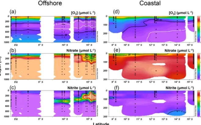
Along the offshore section, the upper oxycline boundary ([O2] =20 µmol L⁻¹ isoline) was at 250–300 m along the Equator at 85.5^◦W, and the ODZ ([O2]<5 µmol L⁻¹) appeared near 10^◦S (Fig. 3a). The southward shoaling of the oxycline, thickening of the ODZ, and shoaling of the [NO⁻₃] =20 µmol L⁻¹isoline were observed south of 10^◦S (Fig. 3a and b), where the thickness of the ODZ was ∼ 300 m. The top of the ODZ reached ∼125 m between 13 and 16^◦S. Significant accumulation of NO⁻₂ (>1 µmol L⁻¹) occurred south of 10^◦S between 30 and 400 m within the ODZ (Fig. 3c), corresponding to lower NO⁻₃ concentrations (Fig. 3b). The highest NO⁻₂ concentration (9.4 µmol L⁻¹) was recorded at 200 m at 15.7^◦S.

Along the coastal section, the surface (upper 10 m) O₂ concentrations were below saturation at all sampling stations (50 %–97 % saturation). Surface O2 concentrations were 165–217 µmol L⁻¹ north of 10^◦S and gradually decreased to 135–190 µmol L⁻¹ between 10 and 12.5^◦S and to 120 µmol L⁻¹ south of 14^◦S (Fig. 3d). The shoaling of the[O₂] =20 µmol L⁻¹isoline was observed south of 9^◦S.

The top of the ODZ was found at 200, 150, and 80 m at 11, 12, and 14^◦S, respectively. The surface NO⁻₃ concentrations were 11–23 µmol L⁻¹between 9 and 16^◦S, and the [NO⁻₃] =20 µmol L⁻¹isoline was at 0–20 m (Fig. 3e). Wa- ter column NO⁻₂ concentrations at coastal stations were generally below 1 µmol L⁻¹, with the exception of the station at 14.0^◦S where NO⁻₂ concentrations reached 1.2 µmol L⁻¹ below 200 m (Fig. 3f).

(5)

Figure 3.Water column oxygen(a, d), nitrate(b, e), and nitrite concentrations(c, f)along the offshore(a, b, c)and coastal sections(d, e, f) during October 2015.

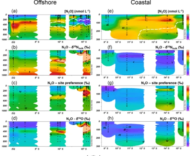
3.2 Water column N2O concentrations and isotopes Along the offshore section, the water column N2O distributions showed a southward increase in surface concentrations and southward decrease in subsurface concentration maxima (Fig. 4a). The equatorial region (1^◦N to 2.5^◦S, 85.5^◦W) had subsurface N₂O concentrations up to 93 nmol L⁻¹ at thermocline depths (200–550 m); water column δ¹⁵N, SP, and δ¹⁸O generally increased with depth (Fig. 4b, c and d); at the subsurface N₂O concentration maximum,δ¹⁵N, SP, and δ¹⁸O were ∼6 ‰, 13 ‰–17 ‰, and 45 ‰–50 ‰, respectively. Two N₂O concentration maxima were observed at stations south of 10^◦S where the ODZ was formed. Near 10^◦S, two N₂O concentration maxima (70±6 nmol L⁻¹) occurred between 200 and 600 m; and a local concentration minimum (∼30 nmol L⁻¹) occurred within the ODZ at 400 m, associated with high δ¹⁵N (8 ‰–10 ‰), SP (20 ‰–30 ‰), and δ¹⁸O (60 ‰–70 ‰). Near 13^◦S, a shallow N2O concentration maximum (∼80 nmol L⁻¹) occurred at∼100 m, and a local N₂O concentration minimum (18 nmol L⁻¹) occurred at 350 m. Between 14 and 16^◦S, the lowest (<10 nmol L⁻¹) N₂O concentrations were observed at 200–400 m within the ODZ, where the highest values ofδ¹⁵N (>10 ‰), SP (30 ‰–

40 ‰), andδ¹⁸O (>60 ‰) were observed.

Along the coastal section, a southward increase in surface N₂O concentration (20 nmol L⁻¹ north of 11^◦S and

>40 nmol L⁻¹ south of 13^◦S) was observed, coinciding with southward shoaling of the ODZ (Fig. 4e). Subsurface

maximum N2O concentrations were observed below 200 m near 10.7^◦S and at 80–90 m south of 12^◦S, where ODZ was formed. The δ¹⁵N values in coastal waters were between 2.5 and 5 ‰, with lower values at stations south of 14^◦S (Fig. 4f). SP was lower (−10 ‰ to 0 ‰) at the surface (<10 m) near 9^◦S and at 50–150 m near 11^◦S; higher SP (10 ‰–20 ‰) was observed south of 14^◦S (Fig. 4g). The δ¹⁸O values were 45 ‰–60 ‰; higherδ¹⁸O (>55 ‰) values were observed within the ODZ below 200 m at 14^◦S and below 100 m at 15.3^◦S (Fig. 4h).

3.3 Excess N₂O and N₂O flux to the atmosphere Both the offshore and coastal stations showed N₂O supersaturation in the top 10 m of surface water, and coastal stations had higher 1N2O concentrations (15–50 nmol L⁻¹) than those of offshore stations (4–8 nmol L⁻¹). Subsurface1N2O along the offshore section had higher concentrations at the equatorial regions (70–80 nmol L⁻¹) than1N2O concentrations at stations located south of 10^◦S (40–60 nmol L⁻¹, Fig. 5a). Near 15^◦S, subsurface N₂O undersaturation was observed;1N₂O concentrations were −4 to 0 nmol L⁻¹ at thermocline depths (200–400 m) within the ODZ ([O₂]<

5 µmol L⁻¹). Along the coastal section, a southward increase in surface and subsurface (50–200 m)1N₂O was observed (Fig. 5b). Subsurface maximum1N₂O concentrations were

>60 nmol L⁻¹, and occurred at the periphery of ODZ (∼ 200 m near 10^◦S and <100 m south of 12^◦S). Undersat-

(6)

Figure 4.Water column N₂O concentrations(a, e),δ¹⁵N_bulk(b, f), site preference(c, g), andδ¹⁸O(d, h)along the offshore(a, b, c, d) and coastal sections(e, f, g, h)during October 2015. White contour lines in(a)and(e)denote the boundary of the oxygen-deficient zone ([O₂] =5 µmol L⁻¹isoline).

uration of N2O (1N2O<0) did not occur in any coastal stations. The N₂O fluxes from the coastal stations were 23–108 µmol m⁻²d⁻¹, nearly 2-fold the offshore fluxes (7–

50 µmol m⁻²d⁻¹, Fig. 5c). The highest flux occurred at a coastal station at 14.4^◦S, 77.3^◦W, coinciding with the highest surface1N₂O (50 nmol L⁻¹).

4 Discussion

The ETSP is one of the world’s major oceanic OMZs having active N2O production and intense efflux to the atmosphere (Arévalo-Martínez et al., 2015; Kock et al., 2016). The gradient spanning from fully oxygenated conditions to anoxia creates suitable conditions for N₂O production and consumption, which causes the coexistence of water column N₂O supersaturation and undersaturation (Codispoti and Chris- tensen, 1985). To identify the N₂O cycling pathways, we input N₂O isotopic and isotopomeric measurements into a simple mass balance model (Sect. 4.1). Quantitative relationships linking O₂, NO⁻₃, and N₂O were examined to char-

acterize the effect of oxygenation on N2O production from NH⁺₄ oxidation (Sect. 4.2). Previously measured N₂O concentrations from the ETSP were extracted from the ME- MENTO database (Kock and Bange, 2015) and were compared to data from this study to investigate the contrasting water column N₂O distribution and effluxes between El Niño and non-El Niño years (Sect. 4.3), which would better con- strain the natural variability of N₂O cycling in the ETSP.

4.1 N₂O cycling pathways inferred from natural abundance isotopic and isotopomeric signatures The analyses of natural abundance isotopomers quantify the substitutions of nitrogen and oxygen isotopes occurring on the linear asymmetric N₂O molecule (Yoshida and Toyoda, 2000), and can be used to identify potential production and consumption pathways (Yamagishi et al., 2007; Grundle et al., 2017). The production of N₂O in an isolated water body follows mass conservation of the respective isotopes and isotopomers. The mass balance model proposed by Fujii et al. (2013) quantified the isotopic signature of N₂O produced

(7)

Figure 5.N₂O excess (1N₂O, nmol L⁻¹) at the offshore section(a)and the coastal section(b)during October 2015; the white dashed line indicates the boundary of the oxygen-deficient zone ([O₂] =5 µmol L⁻¹isoline).(c)Surface N₂O efflux (µmol m⁻²d⁻¹) from offshore and coastal stations (enclosed in white polygon) during October 2015.

within the water mass (δ_produced) by the linear regression of the inverse N₂O concentration (1/[N₂O]_measured) and the observed isotope values (δ_observed):

δ_observed= [N₂O]_initial

[N2O]_measured× δ_initial−δ_produced

+δ_produced, (5)

where[N2O]_initialandδinitialrefer to source water N2O concentration and isotopic signature, respectively. It has been shown that SP is only determined by N2O cycling pathways and that SP is independent of nitrogen isotopic values of the substrates for N₂O cycling. Both culture and field studies demonstrated that N₂O production via NH⁺₄ oxidation and partial denitrification (including both nitrifier- and denitrifier-mediated denitrification) are associated with typi- cal SP values of 30±5 ‰ and 0±5 ‰, respectively (Toy- oda et al., 2011). Recent results from culture (Winther et al., 2018) and river water (Mothet et al., 2013) showed that N₂O production via denitrification had SP values as low as

−10 ‰. Thus, by determining SP_produced, N₂O cycling processes can be qualitatively characterized. We further identified four water bodies (coastal and offshore stations com- bined) from shallow to deeper depths with distinctive features such as O2, NO⁻₂ concentrations, and depths (Table 1) to discuss N₂O cycling pathways as follows.

1. Upper oxycline and surface (Fig. S1a in the Supple- ment): [O₂]>20 µmol L⁻¹,[NO⁻₂]<1 µmol L⁻¹, and

depth<200 m. N₂O production from this water body could actively contribute to atmospheric efflux. The samples had variable SP values (−9 ‰ to 34 ‰); some coastal samples had low SP values (−5 ‰ to −9 ‰, Fig. 4g), which as outlined above is characteristic of strong denitrifying N₂O production. The low SP_produced (6.4±1.9) indicates that both nitrification and denitrification were sources of N₂O to the upper oxycline, with the majority appearing to come from denitrification. Given that the O₂concentrations were too high for denitrification to proceed locally in the upper oxycline and the surface (Codispoti and Christensen, 1985), the SP signature of N2O in this water body was a mixture of local nitrification and denitrification signal from the peak N2O concentration depths (see below) as a result of active upwelling and upward diffusion in the ETSP (Haskell et al., 2015). Thus, denitrification and nitrification both contribute to N₂O effluxes in the ETSP OMZ, consistent with a previous study which focused on the coastal regions between∼12 and 14^◦S (Bourbonnais et al., 2017).

2. N₂O peak (Fig. S1b):[O₂] =5–20 µmol L⁻¹,[NO⁻₂]<

1 µmol L⁻¹, and depth=45–500 m. The samples were from N₂O concentration maxima near the upper boundary of the ODZ. The SP_produced is relatively low (8.3±3.0 ‰) at this suboxic water body ([O₂]<

20 µmol L⁻¹), which allowed N₂O production from

(8)

denitrification while inhibiting N2O consumption (Bonin et al., 1989; Farías et al., 2009). The SP_produced leads us to conclude that water column N₂O maximum was mainly attributed to partial denitrification (i.e., NO⁻₂ and NO⁻₃ reduction). This is consistent with previous¹⁵N tracer incubation experiments demonstrat- ing that N₂O concentration maximum above the ODZ was likely the result of high rates of N₂O production from NO⁻₂ and NO⁻₃ reduction that are 10–100 times higher than the rate of NH⁺₄ oxidation to N₂O (Ji et al., 2015).

3. Oxygen-deficient zone (Fig. S1c): [O2]<5 µmol L⁻¹ and[NO⁻₂]>1 µmol L⁻¹, and depth=70–400 m. The ODZ has prominent features such as the accumulation of NO⁻₂ (Codispoti and Christensen, 1985), and undersaturation of N₂O as a result of dynamic balance between the concomitant N₂O production (Ji et al., 2015) and consumption by denitrification (Babbin et al., 2015). The isotopic signature of “produced N₂O” had distinctively highδ¹⁵N_bulk(8.5 ‰) andδ¹⁸O (71 ‰, Ta- ble 1 and Fig. S2), and this is indicative of pronounced N₂O reduction to N₂, which results in an isotope enrich- ment of the remaining N₂O pool in the process of N–O bond breakage (Toyoda et al., 2017). The SP signature was also high (39.9 ‰). While NH⁺₄ oxidation can pro- duce N2O with similar SP values, we rule this out given the observed low O2concentrations (Peng et al., 2016).

Instead, similar to the high δ¹⁵Nbulk andδ¹⁸O values which were observed, we suggest that the high SP values which were recorded in the ODZ, where N2O undersaturation occurred, were also a result of N₂O consumption, as reduction of N₂O can also result in high SP values (Popp et al., 2002; Well et al., 2005; Mothet et al., 2013). Based on the observedδ¹⁵N_bulk,δ¹⁸O, and SP values of N₂O, we conclude that N₂O consumption was the predominant N₂O cycling pathway in the water body with[O₂]<5 µmol L⁻¹and[NO⁻₂]>1 µmol L⁻¹ in the ETSP.

4. Intermediate waters (Fig. S1d): samples from depths 500–1000 m with [O2] =5–70 µmol L⁻¹ and [NO⁻₂]<1 µmol L⁻¹. Generally, the N2O concentration peak below the ODZ at the offshore waters can be found in this water body (Fig. 4a). From the linear regression, the SPproduced is 15.6±4.1 ‰, indicating that both nitrification and denitrification produced N₂O under the oxic and suboxic conditions ([O₂]=5–

70 µmol L⁻¹). Downward mixing and diffusion from the ODZ is unlikely because the ETSP is a major upwelling region and ODZ samples had high SP values (see next paragraph). We conclude that localized N₂O production from nitrification and denitrification is an important pathway in this region of the water column, and probably contributed to N₂O concentration maxima

in intermediate waters, as reported by Carrasco et al. (2017).

There are some limitations of the isotopomer-based analysis of potential N2O cycling pathways. (1) Constant atmospheric exchange at the surface and mixed layer, and mesoscale eddy activities at intermediate waters (Arévalo- Martínez et al., 2016) could affect the SP_producedfrom localized N₂O cycling. Nevertheless, our conclusion of denitrification being an important pathway remains valid. As a comparison, water bodies were divided by potential density surfaces (i.e.,σ_θ>27, 26–27, 25–26,<25 kg m⁻³) and show- ing SP_producedof 5.0 ‰–11.1 ‰. (2) We are not able to investigate the change in N₂O production rates from nitrification and denitrification that are affected by El Niño-induced lower export production, as demonstrated by Espinoza-Morriberón et al. (2017). With complimentary datasets such as isotopic compositions of NO⁻₃ and NO⁻₂, the rates of N2O production can be derived by isotopic relationships during N2O production processes using a three-dimensional biogeochemical model (Bourbonnais et al., 2017).

4.2 The effect of O₂on N₂O production from NH⁺₄ oxidation

The surface and upper oxycline directly contribute to oceanic N2O effluxes, with NH⁺₄ oxidation being the dominant production pathway due to O2inhibition of denitrification (see Sect. 4.1). Thus, it is worth investigating N2O production from NH⁺₄ oxidation occurring along the oxygen gradient.

During NH⁺₄ oxidation to NO⁻₂, the effectiveness of N2O production can be quantified with the N₂O yield, which is defined as the molar nitrogen ratio of N₂O produced and NH⁺₄ oxidized. In oxygenated waters, the near absence of NH⁺₄ and NO⁻₂ suggests the amount of NH⁺₄ oxidized produces equal amounts of NO⁻₃ within measurement error. Rees et al. (2011) and Grundle et al. (2012) computed the N₂O yield by deriving the slope of the linear regression of the 1N₂O−NO⁻₃ relationship. The 1N₂O data from all sampling stations during October 2015 showed that 1N₂O increases with increasing NO⁻₃ concentrations and decreasing O2 concentrations (Fig. 6). The samples from the upper oxycline ([O2]>20 µmol L⁻¹and depth>500 m) showed a moderate increase in1N2O (0–20 nmol L⁻¹) when [NO⁻₃]<20 µmol L⁻¹. At [NO⁻₃]>20 µmol L⁻¹, substan- tial increase in1N2O (20–75 nmol L⁻¹) was observed. Here, to avoid sampling the ODZ where suboxic conditions stim- ulate N₂O production from partial denitrification (i.e., water body no. 3 described in Sect. 4.1), only data from the upper oxycline (depth<500 m) were used to perform linear regression. The slope of the regression at [NO⁻₃]<20 µmol L⁻¹ (corresponding to[O₂]>100 µmol L⁻¹) is 0.85±0.11, indicating that 0.085±0.011 nmol of N₂O is produced for every micromole of NO⁻₃ produced (or NH⁺₄ oxidized), equat- ing a molar nitrogen yield (mol N₂O-N produced/mol NO⁻₃

(9)

Table 1.Isotopic signature of N₂O cycling processes estimated by linear regression of isotopomer ratios and inverse N₂O concentrations (see Sect. 4.1 for model description and Fig. S1 for results) in water bodies of upper oxycline and surface, N₂O peak, oxygen-deficient zone, and intermediate waters.

No. Layer Definition Statistical properties δ¹⁵N_bulk(‰) δ¹⁸O (‰) SP (‰)

1 Upper oxycline Depth 0–200 m Produced N₂O 2.8 45.9 6.4

and surface [O₂]>5 µmol L⁻¹ Standard error 0.3 1.2 1.9

[NO⁻₂]<1 µmol L⁻¹ R²(n=76) 0.37 0 0.04

2 N₂O peak Depth=45–500 m Produced N₂O 5.4 41.3 8.3

[O₂]=5–20 µmol L⁻¹ Standard error 0.9 3.0 3.0

[NO⁻₂]<1 µmol L⁻¹ R²(n=48) 0.04 0.24 0.08

3 Oxygen-deficient zone Depth=70–400 m Produced N₂O 8.5 71.0 39.9

[O₂]<5 µmol L⁻¹ Standard error 1.5 4.5 4.4

[NO⁻₂]>1 µmol L⁻¹ R²(n=11) 0.38 0.40 0.01

4 Intermediate waters Depth=500–1000 m Produced N₂O 3.6 50.0 15.6

[O₂] =5–70 µmol L⁻¹ Standard error 0.6 2.4 4.1

[NO⁻₂]<0.02 µmol L⁻¹ R²(n=21) 0.69 0 0.04

Figure 6. NO⁻₃–1N₂O relationship for samples from the upper oxycline ([O₂]>20 µmol L⁻¹, depth <500 m, colored circles), low-oxygen ([O₂]<20 µmol L⁻¹) coastal waters (+), low-oxygen offshore waters (open circles), and the lower oxycline (depth >

500 m, filled triangles). Color bar shows the O₂ concentrations (µmol L⁻¹). For samples with NO⁻₃ concentrations higher and lower than 20 µmol L⁻¹, two linear regressions were performed separately.

produced) of 0.17±0.02 %. At[NO⁻₃]>20 µmol L⁻¹(corresponding to [O₂]<100 µmol L⁻¹) the yield increases to 0.85±0.13 %.

These N₂O yield estimates are generally comparable to previously reported values (0.04 %–1.6 %) in the ETSP

(Elkins et al., 1978; Ji et al., 2015), and indicate that potential N₂O production from NH⁺₄ oxidation decreases with water column oxygenation due to intrusion of oxygen-rich water masses (Llanillo et al., 2013; Graco et al., 2017), as well as El Niño-induced oxygenation (see Sect. 4.3). As discussed earlier, the oxycline samples were probably influenced by mixing of suboxic water with active denitrification, produc- ing high N₂O concentrations and low NO⁻₃ concentrations;

the N2O yield estimates here are thus spatially and tempo- rally integrated. As a comparison, the¹⁵N tracer incubation method directly measured 0.04 % N2O yield during NH⁺₄ oxidation at[O2]>100 µmol L⁻¹(Ji et al., 2015).

4.3 N₂O distribution and fluxes during El Niño

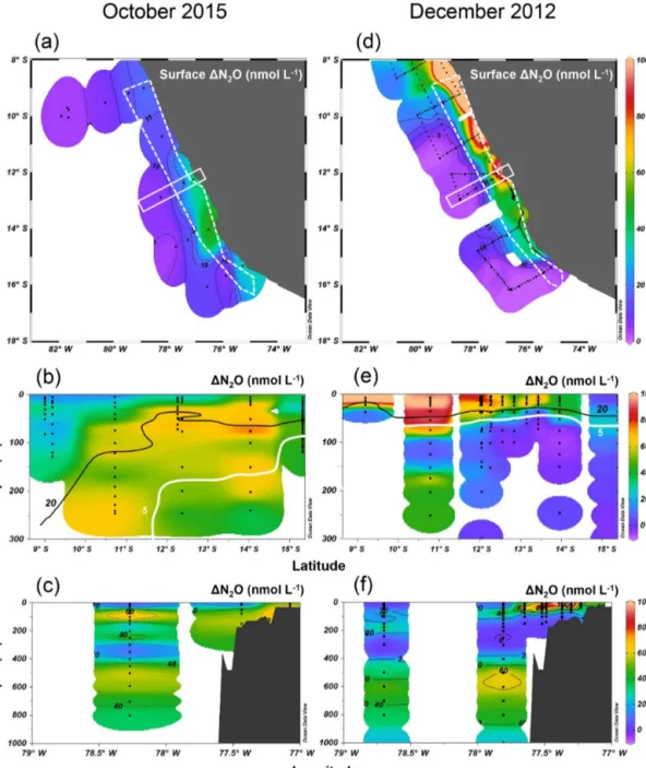
Excess N₂O (1N₂O) in surface waters is one of the prin- cipal factors regulating sea-to-air N₂O fluxes. To evalu- ate the effect of strong El Niño on oceanic N₂O fluxes, we compare surface and water column 1N₂O concentrations in shelf waters (<300 m depth) along 8–16^◦S during El Niño (October 2015) and neutral conditions (Decem- ber 2012). In the ETSP, higher surface 1N2O concentrations and thus higher potential N2O efflux occurred at near- shore waters. Generally, the surface 1N2O concentrations in October 2015 (Fig. 7a) were lower than those of De- cember 2012 (Fig. 7d); the highest surface1N₂O concentrations were 50 and 250 nmol L⁻¹ in 2015 and 2012, respectively. The region of high surface1N₂O occurred near

∼14 and∼10^◦S in 2015 and in 2012, respectively. It ap- pears that N₂O efflux was significantly reduced during El Niño; in October 2015, coastal water had a N₂O flux of 23–

108 µmol m⁻²d⁻¹(Fig. 5c), much lower than that of Decem- ber 2012 having 459–1825 µmol m⁻²d⁻¹(Arévalo-Martínez et al., 2015). Such a 75 %–95 % reduction in N₂O fluxes dur-

(10)

Figure 7.Surface1N₂O(a, d), meridional water column1N₂O distribution(b, e), and zonal water column1N₂O distribution(c, f)in October 2015 and in December 2012. Color bars for1N₂O (nmol L⁻¹) are shown in(d),(e), and(f). For meridional1N₂O distribution(b, e), data are from the coastal section, shown as a white dashed polygon in panels(a)and(d). For zonal1N₂O distribution(c, f), data are from a section 12–13^◦S, shown as a white rectangle. In(b)and(e)the “20” contour line (black) denotes the[O₂] =20 µmol L⁻¹isoline, equivalent to the lower boundary of the oxygenated layer; the “5” contour line (white) denotes the[O₂] =5 µmol L⁻¹isoline, equivalent to the upper boundary of the oxygen-deficient zone.

ing the 2015–2016 El Niño in the ETSP was comparable to an 80 % reduction in fluxes observed in the central equatorial Pacific during the 1982–1983 El Niño (Cline et al., 1987).

Suppressed upwelling or increased downwelling during El Niño events, as observed in both observational and model studies (Llanillo et al., 2013; Graco et al., 2017; Mogollón and Calil, 2017), can directly and indirectly affect N₂O fluxes to the atmosphere: first, reduced upward transport of sub-

surface N2O-rich water not only decreased surface1N2O, but also increased subsurface 1N2O, which is illustrated by the comparative observation of higher subsurface1N2O concentrations in coastal waters in October 2015 (Fig. 7b, c) than those in December 2012 (Fig. 7e, f). Second, because the oxygen sensitivity of the denitrification sequence increases with each step (Körner and Zumft, 1989), El Niño- induced water column oxygenation inhibited N₂O consump-

(11)

Figure 8. Depth profiles of N₂O concentration excess (1N₂O, nmol L⁻¹) measured at six different stations representing offshore (a, b, c)and coastal waters(d, e, f)during February 1985 (filled squares in f), January 2009 (filled triangles in e), Octo- ber 2011 (filled diamonds ind), November 2012 (filled circles ina and b), December 2012 (open squares in c), January 2015 (open circles ineandf), and October 2015 (crosses). Profiles of 2015 are indicated in red and other years in blue. Error bars represent standard deviation of repeated measurements.

tion within the ODZ (bounded by [O₂] =5 µmol L⁻¹ isoline), as demonstrated by the disappearance of N₂O undersaturation (1N₂O<0) in coastal water in 2015 (Fig. 7b, c), contrasting water column N2O undersaturation occurring at 100 m at 13–14^◦S in December 2012 (Fig. 7e, f). Third, as shown in this study, the deepening and expansion of the suboxic zone ([O2] =5–20 µmol L⁻¹) caused by the El Niño event stimulated subsurface N2O production via denitrification, as demonstrated by the close spatial coupling between local maximum 1N₂O concentrations and the oxycline ([O₂] =5 and 20 µmol L⁻¹ isolines, Fig. 7b and e).

Lastly, upwelling of oxygen-rich water along the Peruvian coast, especially north of 12^◦S (Stramma et al., 2016), inhibited local N₂O production and caused the southward relocation of surface1N₂O “hot spots”.

The decrease in surface 1N₂O concentration during El Niño was associated with an increase in subsurface N₂O con-

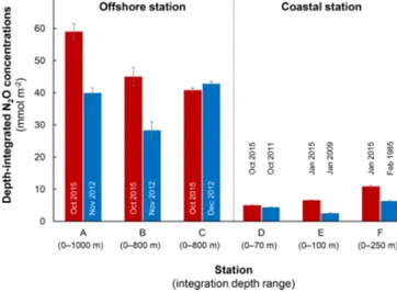
Figure 9.Comparison of depth-integrated N₂O concentrations between El Niño (red bars) and normal years (blue bars). Stations A, B, and C are characterized as offshore stations whereas D, E, and F are coastal stations. Error bars represent propagation of error from analytical precision of respective N₂O concentration profiles. See Fig. 2a for station locations and Table S1 for data sources.

centrations. Water column 1N₂O concentration profiles at expanded temporal and spatial coverage (see Fig. 2a for lo- cation map and Table S1 for coordinates) were compared within the same season between El Niño and non-El Niño years (Fig. 8). We included N2O data from January 2015 when the highest ONI was recorded during austral summer (Fig. 1). These comparisons at offshore stations were made to cover the depth ranges with pronounced El Niño effects and available data (1000 m at station A and 800 m at stations B and C). At coastal stations the depth ranges were station bot- tom depth (stations D and E) or 250 m (station F). Gener- ally, subsurface1N₂O concentration peaks were observed at deeper depths during 2015. Offshore stations had higher subsurface peak1N₂O concentrations during El Niño (Fig. 8a, b), except at station C where the peak concentration during October 2015 was comparable to that of December 2012 (Fig. 8c). At coastal stations D and E, higher 1N₂O concentrations were found below 50 m but peak1N2O concentrations were lower during El Niño years (Fig. 8d, e). At the southernmost coastal station F, the peak1N2O concentration was higher in 2015 than that of 1985; both were found at similar depths at∼60 m. The increase in subsurface N2O concentrations during El Niño resulted in the OMZ water column retaining a larger amount of N₂O, as shown by higher depth-integrated N₂O concentrations during El Niño years than non-El Niño years in both coastal and offshore waters (Fig. 9).

In all, the apparent decrease in N₂O efflux during strong El Niño events in the tropical Pacific, as shown in this study and others (Cline et al., 1987; Butler et al., 1989) is the result of complex physical and biochemical changes. The above

(12)

comparative analyses are simple due to limited data availability. Consequently, these following aspects are yet to be resolved: (1) it is unclear how offshore N₂O fluxes vary from neutral to El Niño years. Current1N₂O profiles show higher surface 1N₂O concentrations at stations A and B in 2015 (Fig. 8a and b), whereas the surface 1N₂O was lower in 2015 at station C (Fig. 8c). A zonal (east–west) section near 12^◦S showed slightly higher offshore surface1N₂O in 2015 (∼5 nmol L⁻¹, Fig. 7c) than in 2012 (∼1 nmol L⁻¹, Fig. 7f).

The decrease in coastal N₂O fluxes during El Niño could be compensated for by increase in offshore fluxes. (2) The southward relocation of high surface1N2O from neutral to El Niño years (Fig. 7a and d) possibly results in higher sur- face1N2O and hence higher N2O flux in the southern region of the ETSP (e.g., south of 16^◦S; Fig. 8f). (3) Complex hy- drographical changes during the El Niño event resulted in the deepening of the ODZ boundary and the depths of peak N₂O concentration. It is possible that these chemical features occur in similar potential density surfaces (with respect to non-El Niño conditions) that are deepened during El Niño, or they occur in different potential density surfaces during El Niño, or a combination of both. (4) It is possible that once the normal upwelling is resumed after the El Niño event, N₂O produced and retained in the subsurface layer in coastal and offshore waters could be a potential reservoir contributing to high N₂O fluxes. (5) The co-occurrence of El Niño and mesoscale eddy formation along the Peruvian coast will have complicated effects on N2O fluxes, which remains un- explored.

5 Conclusions

The eastern tropical South Pacific is a major oceanic upwelling region with N₂O effluxes and active water column production affected by strong El Niño events. During a developing strong El Niño event in October 2015, a more pronounced warming effect occurred at lower latitudes in the ETSP. In comparison to conditions in December 2012 (non- El Niño), deepening of the oxygen-deficient zone’s upper boundary occurred at coastal waters in October 2015, coinciding with lower peak N2O concentrations at deeper depths.

Shelf N2O effluxes were significantly lower during the 2015 El Niño as a result of lower surface levels of N2O supersaturation. However, a change in upwelling pattern appeared to cause higher subsurface N2O concentrations and increased the water column N₂O inventories during El Niño than in other non-El Niño years. Natural abundance isotopic and isotopomeric analysis indicated that both nitrification and denitrification are important pathways for N₂O production, and denitrification-derived N₂O near the suboxic waters probably contributes to the efflux to the atmosphere. Decreased N₂O efflux and subsurface accumulation during strong El Niño events are likely the result of suppressed upwelling and a decrease in water column oxygen consumption. The current

dataset represents a “snapshot” of a developing El Niño event that lasted 18 months; thus the complex spatial and temporal patterns of El Niño-induced N₂O distribution in ETSP remain to be explored.

Data availability. Raw data presented in this paper can be found in the Supplement.

Supplement. The supplement related to this article is available online at: https://doi.org/10.5194/bg-16-2079-2019-supplement.

Author contributions. DSG developed the experimental design and was co-PI and co-chief scientist of the ASTRA-OMZ cruise. HWB, MIG, XM, DLAM, and DSG conducted field sampling. DG, MA, XM, and DLAM conducted laboratory analyses. QJ and DSG performed data synthesis. QJ, MA, HWB, MIG, XM, DLAM, and DSG prepared the paper.

Competing interests. The authors declare that they have no conflict of interest.

Acknowledgements. The German Federal Ministry of Educa- tion and Research (BMBF) grant (03G0243A) awarded to Christa Marandino, Damian Grundle and Tobias Steinhoff supported the ASTRA-OMZ cruise. The BMBF also supported this study as part of the SOPRAN project I and II (03F0611A, 03F0662A). We thank the captain and crew of the R/V Sonne cruise for their technical assistance; Christa Marandino (Chief Sci- entist) and Tobias Steinhoff for co-organizing the R/VSonnecruise with Damian Grundle (co-Chief Scientist); and Martina Lohmann, Hanna Campen and Mingshuang Sun for the oxygen and nutrient measurements and help with N₂O sampling. We thank the Peru- vian authorities for allowing us to conduct work in their territorial waters. We thank Tina Baustian for contributing hydrography and N₂O data off the Peruvian coast. In preparation of the manuscript, Christa Marandino and Lothar Stramma provided constructive com- ments. Qixing Ji received support from the German Science Foun- dation (DFG) grants (GR4731/2-1 and MA6297/3-1) awarded to Damian Grundle and Christa Marandino.

Financial support. This research has been supported by the Ger- man Federal Ministry of Education and Research (BMBF) (grant nos. 03G0243A, 03F0611A, and 03F0662A) and the Deutsche Forschungsgemeinschaft (DFG) (grant Sonderforschungsbereich 754: Climate-Biogeochemistry Interactions in the Tropical Ocean).

The article processing charges for this open-access publication were covered by a Research

Centre of the Helmholtz Association.

(13)

Review statement. This paper was edited by Manmohan Sarin and reviewed by four anonymous referees.

References

Anderson, J. H.: The metabolism of hydroxylamine to nitrite by Nitrosomonas, Biochem. J., 91, 8–17, 1964.

Arévalo-Martínez, D. L., Kock, A., Loscher, C. R., Schmitz, R.

A., and Bange, H. W.: Massive nitrous oxide emissions from the tropical South Pacific Ocean, Nat. Geosci., 8, 530–533, https://doi.org/10.1038/ngeo2469, 2015.

Arévalo-Martínez, D. L., Kock, A., Löscher, C. R., Schmitz, R.

A., Stramma, L., and Bange, H. W.: Influence of mesoscale eddies on the distribution of nitrous oxide in the eastern tropical South Pacific, Biogeosciences, 13, 1105–1118, https://doi.org/10.5194/bg-13-1105-2016, 2016.

Babbin, A. R., Bianchi, D., Jayakumar, A., and Ward, B. B.: Rapid nitrous oxide cycling in the suboxic ocean, Science, 348, 1127–

1129, https://doi.org/10.1126/science.aaa8380, 2015.

Barber, R. T. and Chavez, F. P.: Biological Con- sequences of El Niño, Science, 222, 1203–1210, https://doi.org/10.1126/science.222.4629.1203, 1983.

Blasing, T.: Recent greenhouse gas concentrations, Carbon Diox- ide Information Analysis Center (CDIAC), Oak Ridge National Laboratory (ORNL), Oak Ridge, TN, USA, 2016.

Bonin, P., Gilewicz, M., and Bertrand, J. C.: Effects of oxygen on each step of denitrification on Pseudomonas nautica, Can. J. Mi- crobiol., 35, 1061–1064, https://doi.org/10.1139/m89-177, 1989.

Bourbonnais, A., Letscher, R. T., Bange, H. W., Échevin, V., Larkum, J., Mohn, J., Yoshida, N., and Altabet, M.

A.: N₂O production and consumption from stable isotopic and concentration data in the Peruvian coastal upwelling system, Global Biogeochem. Cy., 31, 678–698, https://doi.org/10.1002/2016GB005567, 2017.

Butler, J. H., Elkins, J. W., Thompson, T. M., and Egan, K.

B.: Tropospheric and dissolved N₂O of the west Pacific and east Indian Oceans during the El Niño Southern Oscillation event of 1987, J Geophys. Res.-Atmos., 94, 14865–14877, https://doi.org/10.1029/JD094iD12p14865, 1989.

Carrasco, C., Karstensen, J., and Farias, L.: On the Ni- trous Oxide Accumulation in Intermediate Waters of the Eastern South Pacific Ocean, Front. Mar. Sci., 4, 24, https://doi.org/10.3389/fmars.2017.00024, 2017.

Chavez, F. P., Ryan, J., Lluch-Cota, S. E., and Ñiquen C. M.: From Anchovies to Sardines and Back: Multi- decadal Change in the Pacific Ocean, Science, 299, 217–221, https://doi.org/10.1126/science.1075880, 2003.

Cline, J. D., Wisegarver, D. P., and Kelly-Hansen, K.: Ni- trous oxide and vertical mixing in the equatorial Pacific during the 1982–1983 El Niño, Deep-Sea. Res., 34, 857–873, https://doi.org/10.1016/0198-0149(87)90041-0, 1987.

Codispoti, L. A. and Christensen, J. P.: Nitrification, denitrification and nitrous oxide cycling in the eastern tropical South Pacific ocean, Mar. Chem., 16, 277–300, https://doi.org/10.1016/0304- 4203(85)90051-9, 1985.

Cornejo, M., Murillo, A. A., and Farías, L.: An unaccounted for N₂O sink in the surface water of the eastern subtropical South

Pacific: Physical versus biological mechanisms, Prog. Oceanogr., 137, 12–23, https://doi.org/10.1016/j.pocean.2014.12.016, 2015.

Elkins, J. W., Wofsy, S. C., Mcelroy, M. B., Kolb, C. E., and Kaplan, W. A.: Aquatic sources and sinks for nitrous oxide, Nature, 275, 602–606, https://doi.org/10.1038/275602a0, 1978.

Espinoza-Morriberón, D., Echevin, V., Colas, F., Tam, J., Ledesma, J., Vásquez, L., and Graco, M.: Impacts of El Niño events on the Peruvian upwelling system pro- ductivity, J. Geophys. Res.-Oceans, 122, 5423–5444, https://doi.org/10.1002/2016JC012439, 2017.

Farías, L., Castro-González, M., Cornejo, M., Charpentier, J., Faún- dez, J., Boontanon, N., and Yoshida, N.: Denitrification and nitrous oxide cycling within the upper oxycline of the eastern tropical South Pacific oxygen minimum zone, Limnol. Oceanogr., 54, 132–144, https://doi.org/10.4319/lo.2009.54.1.0132, 2009.

Farías, L., Faúndez, J., Fernández, C., Cornejo, M., Sanhueza, S., and Carrasco, C.: Biological N₂O Fixation in the Eastern South Pacific Ocean and Marine Cyanobacterial Cultures, PLOS ONE, 8, e63956, https://doi.org/10.1371/journal.pone.0063956, 2013.

Frame, C. H. and Casciotti, K. L.: Biogeochemical controls and isotopic signatures of nitrous oxide production by a marine ammonia-oxidizing bacterium, Biogeosciences, 7, 2695–2709, https://doi.org/10.5194/bg-7-2695-2010, 2010.

Fujii, A., Toyoda, S., Yoshida, O., Watanabe, S., Sasaki, K. I., and Yoshida, N.: Distribution of nitrous oxide dissolved in water masses in the eastern subtropical North Pacific and its origin inferred from isotopomer analysis, J. Oceanogr., 69, 147–157, https://doi.org/10.1007/s10872-012-0162-4, 2013.

Garcia, H. E. and Gordon, L. I.: Oxygen solubility in seawater: Better fitting equations, Limnol. Oceanogr., 6, 1307–1312, https://doi.org/10.4319/lo.1992.37.6.1307, 1992.

Graco, M. I., Purca, S., Dewitte, B., Castro, C. G., Morón, O., Ledesma, J., Flores, G., and Gutiérrez, D.: The OMZ and nutrient features as a signature of interannual and low-frequency variability in the Peruvian upwelling system, Biogeosciences, 14, 4601–4617, https://doi.org/10.5194/bg-14-4601-2017, 2017.

Grundle, D. S., Maranger, R., and Juniper, S. K.: Upper Water Column Nitrous Oxide Distributions in the North- east Subarctic Pacific Ocean, Atmos. Ocean, 50, 475–486, https://doi.org/10.1080/07055900.2012.727779, 2012.

Grundle, D. S., Löscher, C. R., Krahmann, G., Altabet, M. A., Bange, H. W., Karstensen, J., Körtzinger, A., and Fiedler, B.: Low oxygen eddies in the eastern tropical North At- lantic: Implications for N₂O cycling, Sci. Rep.-UK, 7, 4806, https://doi.org/10.1038/s41598-017-04745-y, 2017.

Haskell, W. Z., Kadko, D., Hammond, D. E., Knapp, A. N., Prokopenko, M. G., Berelson, W. M., and Capone, D. G.: Up- welling velocity and eddy diffusivity from⁷Be measurements used to compare vertical nutrient flux to export POC flux in the Eastern Tropical South Pacific, Mar. Chem., 168, 140–150, https://doi.org/10.1016/j.marchem.2014.10.004, 2015.

Ji, Q., Babbin, A. R., Jayakumar, A., Oleynik, S., and Ward, B. B.: Nitrous oxide production by nitrification and denitrification in the Eastern Tropical South Pacific oxygen minimum zone, Geophys. Res. Lett., 42, 10755–10764, https://doi.org/10.1002/2015GL066853, 2015.

Kock, A. and Bange, H. W.: Counting the ocean’s greenhouse gas emissions, Eos, 96, https://doi.org/10.1029/2015EO023665, 2015.