AUTOMATED TERMINATION ANALYSIS OF JAVA BYTECODE BY TERM REWRITING
C. OTTO AND M. BROCKSCHMIDT AND C. VON ESSEN AND J. GIESL LuFG Informatik 2, RWTH Aachen University, Germany
Abstract. We present an automated approach to prove termination of Java Bytecode (JBC) programs by automatically transforming them to term rewrite systems (TRSs). In this way, the numerous techniques and tools developed for TRS termination can now be used for imperative object-oriented languages likeJava, which can be compiled intoJBC.
1. Introduction
Termination of TRSs and logic programs has been studied for decades. But as impera- tive programs dominate in practice, recently many results on termination of imperative programs were developed as well (e.g., [2, 3, 4, 5, 12]). Our goal is to re-use the wealth of techniques and tools from TRS termination when tackling imperative object-oriented programs. Similar TRS-based approaches have already proved successful for termination analysis of PrologandHaskell[10, 17]. A first approach to prove termination of imperative programs by transforming them to TRSs was presented in [7]. However, [7] only analyzes a toy programming language without heap, whereas our goal is to analyze JBCprograms.
JBC[14] is an assembly-like object-oriented language designed as intermediate format for the execution ofJava[11] programs by aJava Virtual Machine(JVM). Moreover,JBCis a common compilation target for many other languages besidesJava. While there exist several static analysis techniques for JBC, we are only aware of two other automated methods to analyze termination of JBC, implemented in the tools COSTA [1] and Julia [19]. They transform JBC into a constraint logic program by abstracting every object of a dynamic data type to an integer denoting its path-length (i.e., the maximal length of the path of pointers that can be obtained by following the fields of objects). For example, consider a data structure IntList with the field value for the first list element and the field next which points to the next list element. Now an object of type IntList representing the list [0,1,2] would be abstracted to its length 3, but one would disregard the values of the list elements. While this fixed mapping from data objects to integers leads to a very efficient analysis, it also restricts the power of these methods. In contrast, in our approach we represent data objects not by integers, but by terms. To this end, we introduce a function symbol for every class. So theIntList object above is represented by a term like
Key words and phrases: Java Bytecode, termination, term rewriting.
Supported by the DFG grant GI 274/5-2 and by the G.I.F. grant 966-116.6.
c C. Otto, M. Brockschmidt, C. von Essen, and J. Giesl Confidential — submitted to RTA
IntList(0,IntList(1,IntList(2,null))), which keeps the whole information of the data object.
So compared to [1, 19] and to direct termination analysis of imperative programs, rewrite techniques1 have the advantage that they are very powerful for algorithms on user- defined data structures, since they can automatically generate suitable well-founded orders comparing arbitrary forms of terms. Moreover, by using TRSs with built-in integers [8], rewrite techniques are also powerful for algorithms on pre-defined data types like integers.
Inspired by our approach for termination of Haskell [10], in this paper we present a method to translate JBC programs to TRSs. More precisely, in Sect. 2 we show how to automatically construct a termination graph representing all execution paths of the JBC program. Similar graphs are also used in program optimization techniques, e.g. [18]. While we perform considerably less abstraction than [1, 19], we also apply a suitable abstract interpretation [6] in order to obtain finite representations for all possible forms of the heap at a certain state. In contrast to control flow graphs, the nodes of the termination graph contain not just the current program position, but also detailed information on the values of the variables and on the content of the heap. Thus, the termination graph usually has several nodes which represent the same program position, but where the values of the variables and the heap are different. This is caused by different runs through the program code. The termination graph takes care of all aliasing, sharing, and cyclicity effects in the JBCprogram. This is needed in order to express these effects in a TRS afterwards. Then, a TRS is generated from the termination graph such that termination of the TRS implies termination of the originalJBC program (Sect. 3). The resulting TRSs can be handled by existing TRS termination techniques and tools.
As described in Sect. 4, we implemented the transformation in our toolAProVE[9]. In the firstInternational Termination Competition on automated termination analysis of JBC, AProVE achieved competitive results compared to Julia and COSTA. So this paper shows for the first time that rewriting techniques can indeed be successfully used for termination of imperative object-oriented languages like Java.
2. From JBC to Termination Graphs
To obtain a finite representation of all execution paths, we evaluate the JBC program symbolically, resulting in a termination graph. Afterwards, this graph is used to generate a TRS suitable for termination analysis. Sect. 2.1 introduces the abstract states used in termination graphs. Then Sect. 2.2 illustrates the construction of termination graphs for simple programs and Sect. 2.3 extends it to programs with complex forms of sharing.
2.1. Representing States of the JVM
We defineabstract states which representsets of concreteJVMstates, using a formalization which is especially suitable for a translation into TRSs (see e.g. [13] for related formaliza- tions). Our approach is restricted to verified sequential JBC programs without recursion.
1Of course, one could also use a transformation similar to ours whereJBCis transformed to (constraint) logic programs, but where data objects are also represented by terms instead of integers. In principle, such an approach would be as powerful as ours, provided that one uses sufficiently powerful underlying techniques for automated termination analysis of logic programs. However, since some of the most powerful current termination analyzers for logic programs are based on term rewriting [15, 17], it seems more natural to transformJBCto term rewriting directly.
To simplify the presentation in the paper, we only consider program runs involving a single method, and exclude floating point arithmetic, arrays, exceptions, and static class fields.
However, our approach can easily be extended to such constructs and to arbitrary many non-recursive methods. For the latter, we represent the frames of the call stack individually and simply “inline” the code of invoked methods. Indeed, our implementation also handles programs with several methods including floats, arrays, exceptions, and static fields.
Definition 2.1. The set of abstract states isStates=ProgPos×LocVar×OpStack×Heap. The first component of a state corresponds to the program counter. We represent it by the next program instruction to be executed (e.g., by a JBCinstruction like “ifnull 8”).
The second component is an array of the local variables which have a defined value at the current program position, represented by a partial functionLocVar=N→References. Here, References are addresses in the heap. So in our representation, we do not store primitive values directly, but indirectly using references to the heap. This enables us to re- tain equality information for two otherwise unknown primitive values. Moreover, we require null∈Referencesto represent the nullreference. To ease readability, in examples we usually denote local variables by names instead of numbers. Thus, “o:o1,l:o2” denotes an array where the 0-th local variable oreferences the address o1 in the heap and the 1-st local variable l references the address o2 in the heap. Of course, different local variables can point to the same address (e.g., in “o:o1,l:o2,c:o1”,oandcrefer to the same object).
The third component is the operand stack thatJBCinstructions operate on. It will be filled with intermediate values such as operands of arithmetic operations when evaluating the bytecode. We represent it by a partial function OpStack=N→ References. The empty operand stack is denoted by “ε” and “i1, i2” denotes a stack with top elementi2.
ifnull 8|o:o1,l:o2|o1
o1=Int(val=i1) i1 = (−∞,∞) o2=Int(?)
Figure 1: An abstractJVMstate
To depict abstract states in examples, we write the first three components in the first line and separate them by “|”. The fourth Heap component is written in the lines below, cf. Fig. 1. It describes the values of References. We represent the Heap by a partial functionHeap:References→Integers ∪ Instances ∪ Unknown.
The values inUnknown=Classnames×{?}represent tree-shaped (and thus acyclic) objects for which we have no information except their type. Classnames contains the names of all classes and interfaces of the program. So for a classInt, “o2 =Int(?)” means that the object at address o2 is nullor an instance of typeInt (or a subtype ofInt).
We represent integers as possibly unbounded intervals, i.e. Integers={{x ∈Z|a≤ x ≤ b} | a∈ Z∪ {−∞}, b ∈ Z∪ {∞}, a ≤b}. Soi1 = (−∞,∞) means that any integer can be at the address i1. Since current TRS termination tools cannot handle 32-bit int- numbers as in JBC, we treat int as the infinite set of all integers, i.e., we cannot handle problems related to overflows. Note that inJBC,int is also used for Boolean values.
To represent Instances (i.e., objects) of some class, we describe the values of their fields, i.e., Instances=Classnames×(FieldIdentifiers→References). To prevent ambiguities, in general the FieldIdentifiers also contain the respective class names. So if the classInthas the fieldvalof typeint, then “o1 =Int(val=i1)” means that at the address o1, there is an instance of class Int and its field val references the address i1 in the heap. Note that all sharing and aliasing must be explicitly represented in the abstract state. So since the state in Fig. 1 contains no sharing information foro1 and o2,o1 and the references reachable fromo1 are disjoint fromo2 and from the references reachable fromo2.
00: aload_0 // load orig to opstack 01: ifnull 8 // jump to line 8 if top
// of opstack is null 04: aload_1 // load limit
05: i f n o n n u l l 9 // jump if not null 08: return
09: aload_0 // load orig 10: astore_2 // store into copy 11: aload_0 // load orig 12: getfield val // load field val 15: aload_1 // load limit 16: getfield val // load field val 19: i f _ i c m p g e 35 // jump if
// orig . val >= limit . val 22: aload_2 // load copy
23: aload_2 // load copy 24: getfield val // load field val 27: iconst_1 // load constant 1 28: iadd // add copy . val and 1 29: putfield val // store into copy . val 32: goto 11
35: return
(a) Java Bytecode
p u b lic c l a s s I n t {
// o n l y wrap a p r i m i t i v e i n t p r i v a t e i n t v a l ;
// c o u nt up t o t h e v a l u e // i n ” l i m i t ”
p u b lic s t a t i c void c o u n t ( I n t o r i g , I n t l i m i t ) {
i f ( o r i g == n u l l
| | l i m i t == n u l l) { return;
}
// i n t r o d u c e s h a r i n g I n t copy = o r i g ;
while ( o r i g . v a l < l i m i t . v a l ) { copy . v a l ++;
} } }
(b)Java Source Code
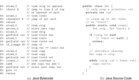
Figure 2: Example using aliasing and an integer counting upwards 2.2. Termination Graphs for Simple Programs
We now introduce the termination graph using a simple example. In Fig. 2(a) we present the analyzed JBCprogram and Fig. 2(b) shows the corresponding Java source code.
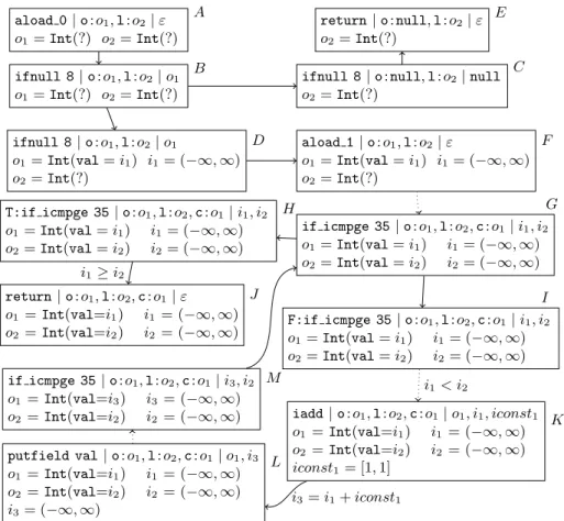
We create the termination graph using the states of a run of our abstract virtual machine as nodes, starting in a suitable general state. In our example, we want to know ifall calls of the methodcountwith two distinct arbitraryIntobjects (ornull) as arguments terminate.
Here it is important to handle the aliasing of the variables copyand orig.
In Fig. 3, node A contains the start state. For the local variables orig and limit (abbreviated oand l), we only know their type and we know that they do not share any part of the heap. The firstJBCinstructionaload 0loads the value of the 0-th local variable (the argument orig) on the operand stack. The variable origreferences some address o1
in the heap, but we do not need concrete information about o1 for this instruction. The resulting new state B is connected to Aby an evaluation edge.
To evaluate the ifnull instruction, we need to know if the reference on top of the operand stack is null. This is not yet known foro1. We refine the information and create successor nodes C and D for all possible cases (i.e., for o1 == null, and for Int and all its non-abstract subclasses). In C, o1 is null, and in D it is an instance of Int (Int has no proper subtypes). In D, the field values are new references in the heap. So instead of
“o1 =Int(?)”, we now have “o1 =Int(val=i1)”. Note that while “o1 =Int(?)” in nodeB means that ifo1 is notnull, then it has typeIntor a subtype of it, “o1 =Int(val=i1)”
in node D means that o1’s type is exactly Int and not a proper subtype. We have no information about the value ati1. Therefore,i1 gets the most general value for Integers, i.e., i1= (−∞,∞). C and Dare connected to B byrefinement edges.
Now we can evaluate the instruction both forC andD, leading toE andF. Evaluation stops inE, while forF, the same procedure is repeated for the argumentlimit, leading to node G(among others) after several steps, indicated by a dotted arrow. Note the aliasing betweencopyand orig, since both reference the same object at the address o1.
aload 0|o:o1,l:o2 |ε o1=Int(?) o2=Int(?)
A
ifnull 8|o:o1,l:o2|o1
o1=Int(?) o2=Int(?)
B ifnull 8|o:null,l:o2|null o2=Int(?)
C return|o:null,l:o2|ε o2=Int(?)
E
ifnull 8|o:o1,l:o2|o1
o1 =Int(val=i1) i1= (−∞,∞) o2 =Int(?)
D aload 1|o:o1,l:o2|ε
o1=Int(val=i1) i1= (−∞,∞) o2=Int(?)
F
if icmpge 35|o:o1,l:o2,c:o1|i1, i2
o1=Int(val=i1) i1 = (−∞,∞) o2=Int(val=i2) i2 = (−∞,∞) T:if icmpge 35|o:o1,l:o2,c:o1|i1, i2 G
o1=Int(val=i1) i1 = (−∞,∞) o2=Int(val=i2) i2 = (−∞,∞)
H
return|o:o1,l:o2,c:o1|ε o1 =Int(val=i1) i1 = (−∞,∞) o2 =Int(val=i2) i2 = (−∞,∞)
J
F:if icmpge 35|o:o1,l:o2,c:o1|i1, i2
o1 =Int(val=i1) i1= (−∞,∞) o2 =Int(val=i2) i2= (−∞,∞)
I
iadd|o:o1,l:o2,c:o1|o1, i1, iconst1
o1 =Int(val=i1) i1 = (−∞,∞) o2 =Int(val=i2) i2 = (−∞,∞) iconst1= [1,1]
K putfield val|o:o1,l:o2,c:o1|o1, i3
o1 =Int(val=i1) i1 = (−∞,∞) o2 =Int(val=i2) i2 = (−∞,∞) i3= (−∞,∞)
L if icmpge 35|o:o1,l:o2,c:o1|i3, i2
o1 =Int(val=i3) i3 = (−∞,∞) o2 =Int(val=i2) i2 = (−∞,∞)
M i1≥i2
i1 < i2
i3=i1+iconst1
Figure 3: Termination graph for count
InG, we have already evaluated the two “getfield val” instructions and have pushed the two integer values on the operand stack. Now if icmpge requires us to compare the unknown integers ati1 andi2. If we had to comparei1 with a fixed number like 0, we could refine the information abouti1 and i2 and create two successor nodes with i1 = (−∞,−1]
and i1 = [0,∞). But “i1 ≥ i2” is not expressible in our abstract states. Here, we split according to both possible values of the condition (depicted using the labels “T” and “F”, respectively). This leads to the nodes H and I which are connected toGby split edges.
We can evaluate the condition inH to trueand label the resulting evaluation edge to J by this condition. We will use these labels when constructing a TRS from the termination graph. J marks the program end and thus, it remains a leaf of the graph.
In I, we can evaluate the condition to false and label the next edge by the converse of the condition. After evaluating the next four instructions we reach nodeK. On the top positions of the operand stack, there are two integer variables (where the topmost variable has the value 1). The instructioniadd adds these two variables resulting in a new integer variable i3. The relation betweeni3, i1, and iconst1 is added as a label on the evaluation edge to the new node L. This label will again be used in the TRS construction.
From Lon, we evaluate instructions until we again arrive at the instructionif icmpge in node M. It turns out that M is an instance of the previous node G. Hence, we can connect M withG by aninstantiation edge. The reason is that every concrete state which would be described by the abstract stateM could also be described by the stateG.
One has to expand termination graphs until all leaves correspond to program ends.
Hence, our graph is now completed. By using appropriate generalization steps (which transform nodes into more general ones), one can always obtain a finite termination graph.
To this end, one essentially executes the program symbolically until one reaches some posi- tion in the program for the second time. Then, a new state is created that is a generalization of both original states and one introduces instantiation edges from the two original states to the new generalized state. Of course, in our implementation we apply suitable heuristics to ensure that one only performs finitely many such generalization steps and to guarantee that the construction always terminates with a finite termination graph.
To define “instance” formally, we first define all positionsπ of references in a state s, wheres|π denotes the reference at position π. A positionπ is a sequence starting with lvn or osn for some n ∈ N (indicating the n-th reference in the local variable array or in the operand stack), followed by zero or more FieldIdentifiers.
Definition 2.2 (position, SPos). Let s = (pp, l, op, h) ∈ States. Then SPos(s) is the smallest set such that one of the following holds for allπ ∈SPos(s):
• π=lvn for somen∈Nwhere l(n) is defined. Then s|π isl(n).
• π=osn for somen∈Nwhereop(n) is defined. Then s|π isop(n).
• π =π′v for some v ∈FieldIdentifiers and some π′ ∈ SPos(s) where h(s|π′) = (c, f)∈Instances and wheref(v) is defined. Thens|π isf(v).
As an example, consider the state s depicted in node G of Fig. 3. Here we have three local variables and two elements on the operand stack. Thus, SPos(s) contains lv0,lv1,lv2,os0,os1, where s|lv0 = s|lv2 = o1, s|lv1 = o2, s|os0 = i1, and s|os1 = i2. If h is the heap of that state, then h(o1) = (Int, f1) ∈ Instances, where f1(val) = i1. Hence, “lv0val” is also a position in SPos(s) and s|lv0val =i1. The remaining elements of SPos(s) are “lv2val” and “lv1val”, wheres|lv2val =i1 and s|lv1val=i2.
Intuitively, a states′ is an instance of a statesif they correspond to the same program position and whenever there is a references′|π, then either the values represented bys′|π in the heap of s′ are a subset of the values represented bys|π in the heap ofsor else, π is no position ins. Moreover, shared parts of the heap ins′ must also be shared ins. Note that sincesands′ correspond to the same position in averified JBCprogram,sands′ have the same number of local variables and their operand stacks have the same size.
Definition 2.3 (Instance). We say that s′ = (pp′, l′, op′, h′) is an instance of state s = (pp, l, op, h) (denoted s′ ⊑s) iffpp=pp′, and for all π, π′ ∈SPos(s′):
(a)ifs′|π =s′|π′ andh′(s′|π)∈Instances∪Unknown, thenπ, π′∈SPos(s) ands|π=s|π′
(b) ifs′|π 6=s′|π′ and π, π′ ∈SPos(s), thens|π 6=s|π′
(c) ifh′(s′|π)∈Integersand π ∈SPos(s), then h(s|π)∈Integersandh′(s′|π)⊆h(s|π) (d) ifs′|π =nulland π∈SPos(s), thens|π =nullorh(s|π) = (c,?)∈Unknown
(e) ifh′(s′|π) = (c′,?) and π∈SPos(s), thenh(s|π) = (c,?) where c′ is cor a subtype of c (f) ifh′(s′|π) = (c′, f′)∈Instancesand π∈SPos(s), then h(s|π) = (c′, f)∈Instances
orh(s|π) = (c,?), wherec′ must be cor a subtype of c.
The state s′ in nodeM of Fig. 3 is an instance of the state sin nodeG. Clearly, they both refer to the same program position. It remains to examine the references reachable ins′. We haveSPos(s′) =SPos(s) ={lv0,lv1,lv2,os0,os1,lv0val,lv1val,lv2val}. It is easy to check that the conditions of Def. 2.3 are satisfied for all these positions π. We illustrate this for π = lv0val. Here, s′|π = i3 and if h′ is the heap of s′, then h′(i3) =
(−∞,∞). Similarly, s|π =i1 and if his the heap of s, thenh(i1) = (−∞,∞). Here,s′ and sare in fact equivalent, sinceM is an instance of Gand Gis an instance of M.
if icmpge35|o:o1,l:o2,c:o1|i1, i2
o1 =Int(val=i1) i1 = [1,1]
o2 =Int(val=i2) i2 = [10000,10000]
Figure 4: A concrete state
As remarked before, abstract states describe sets of concrete states like the one in Fig. 4, which is an instance of G and M. Here, the values for i1 and i2 are proper integers instead of intervals.
Definition 2.4(Concrete state). A states= (pp, l, op, h) isconcrete if for allπ ∈SPos(s):
• h(s|π)∈/Unknownand
• ifh(s|π)∈Integers, thenh(s|π) is just a singleton interval [i, i] for somei∈Z A concrete state has no proper instances (i.e., if sis concrete ands′ ⊑s, thens⊑s′).
Concrete states that are not a program end can always be evaluated and have exactly one (concrete) successor state. For Fig. 4, sincei1’s value is not greater or equal thani2’s, the successor state corresponds to the instruction “aload 2”, with the same local variables and empty operand stack. Such a sequence of concrete states, obtained by JBC evaluation, is called acomputation sequence. Our construction of termination graphs ensures that
if s is an abstract state in the termination graph and there is a con- crete state t ⊑ s where t evaluates to the concrete state t′, then the termination graph contains a path fromsto a state s′ with t′⊑s′.
(2.1) To see why (2.1) holds, note that in the termination graph,sis first refined to a stateswith t⊑s. So there is a path fromstos, and in the states, all concrete information needed for an actual evaluation according to theJBCspecification [14] is available. Note that “evaluation edges” in the termination graph are defined by exactly following the specification of JBC in [14]. Thus, there is an evaluation edge fromsto s′, wheret′ ⊑s′.
The computation sequence from Fig. 4 to its concrete successor corresponds to the path from node M or G to I’s successor. Paths in the graph that correspond to computation sequences are called computation paths. Our goal is to show that all these paths are finite.
Definition 2.5 (Graph termination). A finite or infinite path s11, . . . , sn11, s12, . . . , sn22, . . . through the termination graph is called a computation path iff there is a computation sequence t1, t2, . . . of concrete states where ti ⊑s1i for all i. A termination graph is called terminatingiff it has no infinite computation path. Note that due to (2.1), if the termination graph is terminating, then the original JBC program is also terminating for all concrete states twheret⊑sfor some abstract state sin the termination graph.
2.3. Termination Graphs for Complex Programs
Now we discuss sharing problems in complex programs with recursive data types. In Fig. 5, flattentakes a list of binary trees whose nodes are labeled by integers. It performs a depth- first run through all trees and returns the list of all numbers in these trees. It terminates because each loop iteration decreases the total number of all nodes in the trees of list, even though list’s length may increase. Note that listand curshare part of the heap.
Consider the three states A, B, and C in Fig. 6. A is the state of our abstract JVM when it first reaches the loop condition “cur != null” (where list,cur, and resultare abbreviated byl,c, and r). After one execution of the loop body, one obtains the state B iftreeisnulland Cotherwise. Note that local variables declared in the loop body are no longer defined at the loop condition, and hence, they do not occur in A,B, orC.
p u b lic c l a s s F l a t t e n {
p u b lic s t a t i c I n t L i s t f l a t t e n ( T r e e L i s t l i s t ) { T r e e L i s t c u r = l i s t ;
I n t L i s t r e s u l t = n u l l; while ( c u r != n u l l) {
Tree t r e e = c u r . v a l u e ; i f ( t r e e != n u l l) {
I n t L i s t o l d I n t L i s t = r e s u l t ; r e s u l t = new I n t L i s t ( ) ; r e s u l t . v a l u e = t r e e . v a l u e ; r e s u l t . n e x t = o l d I n t L i s t ; T r e e L i s t o l d Cu r = c u r ; c u r = new T r e e L i s t ( ) ; c u r . v a l u e = t r e e . l e f t ; c u r . n e x t = o l d Cu r ;
o l d Cu r . v a l u e = t r e e . r i g h t ; } e l s e c u r = c u r . n e x t ; }
return r e s u l t ; }
}
p u b lic c l a s s Tree { i n t v a l u e ;
Tree l e f t ; Tree r i g h t ; }
p u b lic c l a s s T r e e L i s t { Tree v a l u e ;
T r e e L i s t n e x t ; }
p u b lic c l a s s I n t L i s t { i n t v a l u e ;
I n t L i s t n e x t ; }
Figure 5: Example converting a list of binary trees to a list of integers
aload 1|l:o1,c:o1,r:null|ε o1 =TreeList(?)
A
aload 1|l:o1,c:o3,r:null|ε o1 =TreeList(value=null,next=o3) o3 =TreeList(?)
B
aload 1|l:o1,c:o7,r:o6|ε o1 =TreeList(value=o5,next=o3) o3 =TreeList(?) o5 =Tree(?) o6 =IntList(value=i1,next=null) o7 =TreeList(value=o4,next=o1) i1= (−∞,∞) o4 =Tree(?) C
Figure 6: Three states of the termination graph offlatten
If one continued the evaluation like this, one would obtain an infinite tree, since one never reaches any state which is an instance of a previous state. (In particular, B and C are no instances of A.) Hence, to obtain finite graphs, one sometimes has to generalize states. Thus, we want to create a new general stateS such thatA,B, andC are instances of S. Note that in S, land c cannot point to different references with Unknownvalues, since then S would only represent states where l and c are tree-shaped and not sharing.
However,landcpoint to thesame object inA, one can reachc:o3 froml:o1 inB (i.e.,l joins c, since a field value ofo1 iso3), and one can reach l:o1 from c:o7 inC. To express such sharing information in general states, we extend states byannotations.
o o′
o1 =? o2
o o′
o1
o o′
o1 o2
Figure 7: “=?” annotation
In Fig. 7, the leftmost picture depicts a heap where an instance referenced by o has a field value o1 and o′ has a field value o2. The annotation
“o1 =? o2” means that o1 and o2 could be equal.
Here the value of at least one of o1 and o2 must be Unknown. So both the second and the third shape in Fig. 7 are instances of the first. In the second shape, o1 and o2 are equal and all occur- rences ofo2 can be replaced by o1 (or vice versa). In the third shape,o1 ando2 are not the same and thus, the annotation has been removed.
o1 %$ o2
o1 o2
o1 o2
o1 o2
o3 o4
Figure 8: “%$” annotation So the =? annotation covers both the equality
oflandcin stateAand their non-equality in states B and C. To represent states wherel and cmay join, we use the annotation “%$”. We say that a
reference o′ is adirect successor of a reference o(denoted o→ o′) iff the object at address o has a field whose value is o′. As an example, consider state B in Fig. 6, where o1 → o3
holds. Then the annotation “o1 %$ o2” means that ifo1 isUnknown, then there could be an object o with o1 →+ o and o2 →∗ o, i.e., o is a proper successor of o1 and a (possibly non-proper) successor of o2. Note that %$ is symmetric,2 soo1 %$ o2 also means that ifo2 isUnknown, then there could be an object o′ witho1→∗ o′ ando2 →+o′. The shapes 2-4 in Fig. 8 visualize three possible instances of the state with annotation “o1 %$ o2”. Note that a state in whicho1 and o2 do not share is also an instance.
We can now create a state S (see Fig. 9) such thatA, B, C⊑S. The annotations state thatland cmay be equal (as inA), thatlmay joinc(as inB), orcmay joinl(as inC).
So to obtain a finite termination graph, after reachingA, we generalize it to a new node S connected by an instantiation edge. As seen inD, we introduce new forms of refinement edges to refine a state with the annotation “o1 =?o7” into the two instances whereo1 =o7
and where o1 6= o7. For o1 = o7, we reach B′ and C′ which are like B and C but now r points to a list ending witho6 instead ofnull. The nodesB′ and C′ are connected back to S with instantiation edges. For o1 6=o7, due toc != null, we first refine the information about o7, and obtain o7 =TreeList(value=o8,next=o9). Note that “%$” annotations have to be updated during refinements. If we have the annotation “o1 %$ o7” and if one refines o7 by introducing references like o8, o9 for its non-primitive fields, then we have to add corresponding annotations such as “o1 =?o9” for all field references likeo9 whose types correspond to the type ofo1. Moreover, we add “%$” annotations for all non-primitive field references (i.e., “o1 %$ o8” and “o1 %$ o9”). If after this refinement neither o1 nor o7 were Unknown, we would delete the annotation o1 %$ o7 since it has no effect anymore.
A aload 1|l:o1,c:o7,r:o6|ε
o1 =TreeList(?) o6 =IntList(?) o7 =TreeList(?)
o1=?o7 o1%$o7
S
D
B′ C′
putfield value|l:o1,c:o13,r:o12,t:o8,oIL:o6,oC:o7|o7, o11
o1=TreeList(?) o9=TreeList(?) o6 =IntList(?) o7 =TreeList(value=o8,next=o9) o10 =Tree(?) o8 =Tree(value=i1,left=o10,right=o11)o11 =Tree(?) o12=IntList(value=i1,next=o6) i1 = (−∞,∞) o13=TreeList(value=o10,next=o7) o1=?o9
o1%$o7 o1%$o8 o1%$o9 o1%$o10 o1%$o11
F aload 1|l:o1,c:o13,r:o12|ε
o1 =TreeList(?) o6 =IntList(?) o9 =TreeList(?) o7 = TreeList(value=o11 ,next=o9) o10 =Tree(?) o12= IntList(value=i1,next=o6) o11 =Tree(?) o13= TreeList(value=o10,next=o7) i1 = (−∞,∞) o1=?o9 o1%$o7 o1%$o9 o1%$o10 o1%$o11
G
aload 1|l:o1,c:o9,r:o6 |ε
o1 =TreeList(?) o6 =IntList(?) o9 =TreeList(?)
o1 =?o9 o1%$o9
E
o1=o7
o16=o7
Figure 9: Termination graph forflatten
Now we use a refinement that corresponds to the case analysis whether treeis null.
For tree == null, after one loop iteration we reach nodeE which is again an instance of S. Here, the local variabletreeis no longer visible.
2Since both “=?” and “%$” are symmetric, we do not distinguish between “o1 =? o2” and “o2 =? o1” and we also do not distinguish between “o1 %$ o2” and “o2 %$ o1”.
For tree != null, the graph shows nodes F and G. In F we need to evaluate a putfield instruction (corresponding to “oldCur.value = tree.right”), i.e., we have to put the object at address o11 to the field value of the object at addresso7. The effect of this operation can be seen in the box in state G, where the value of the object at o7 was changed fromo8 too11. InG(which again corresponds to the loop condition), we removed the referenceo8 since it is no longer accessible from the local variables or the operand stack.
In contrast to other evaluation steps, suchputfieldinstructions can give rise to addi- tional annotations, since objects that already shared parts of the heap witho7now may also share parts of the heap with o11. We say that a reference o reaches a reference o′ iff there is a successorr of o(i.e.,o→∗ r) such thatr =o′ orr=?o′ orr %$o′. So in our example, o11 reaches just o11 and o1. Now if we write o11 to a field of o7, then for all references o witho%$ o7, we have to add the annotation o%$ o′ for all o′ whereo11 reaches o′. Hence, in our example, we would have to addo1 %$ o11(which is already present in the state) and o1 %$ o1. However, the annotation o1 %$ o1 has no effect, since by “o1 = TreeList(?)”, we know that o1 only represents tree-shaped objects. Therefore, we can immediately drop o1 %$ o1 from the state. Concrete non-tree-shaped objects can of course be represented easily (e.g., “o=TreeList(value=o′,next=o)”). But to represent anarbitrary possibly non-tree-shaped objecto, we use a special annotation (depicted “o!”).3
Definition 2.6 (Instance & annotations). We extend Def. 2.3 to s, s′ = (pp′, l′, op′, h′) ∈ States possibly containing annotations. Nows′ ⊑s holds iff for all π, π′ ∈SPos(s′), the following conditions are satisfied in addition to Def. 2.3 (b)-(f). Here, let τ resp. τ′ be the maximal prefix ofπ resp.π′ such that bothτ, τ′ ∈SPos(s).
(a) ifs′|π =s′|π′ where h′(s′|π)∈Instances∪Unknown, and if π, π′ ∈SPos(s),4 then s|π =s|π′ ors|π =? s|π′
(b) ifs′|π =?s′|π′ and π, π′ ∈SPos(s), then s|π =?s|π′
(c) if s′|π =s′|π′ whereh′(s′|π)∈Instances∪Unknown, or s′|π =? s′|π′ and π orπ′ 6∈SPos(s) with π6=π′, thens|τ %$ s|τ′
(d) ifs′|π %$s′|π′, then s|τ %$ s|τ′ (e) ifs′|π! holds, then s|τ!
(f) if there exist (possibly empty) sequences ρ6=ρ′ of FieldIdentifiers without common prefix, wheres′|πρ=s′|πρ′, h′(s′|πρ)∈Instances∪Unknown,
and (πρ orπρ′ 6∈SPos(s) or s|πρ=?s|πρ′), then s|τ!
3. From Termination Graphs to TRSs
Now we transform termination graphs into integer term rewrite systems (ITRSs). These are TRSs where the Booleans B, the integers Z, and their built-in operations ArithOp = {+,−,∗, /,%,≪,≫,≫,b,&,| } and RelOp = {>,≥, <,≤,==,6=} are pre-defined by an infinite set of variable-free rulesPD. For example,PDcontains1+2→3and5<4→false.
As shown in [8], TRS termination techniques can easily be adapted to ITRSs as well.
3Such annotations can also result fromputfieldoperations which write a referenceo2 to a fieldfofo1. If o1 already reached o2 before through some fieldg 6=f, then we add “o1!”, since o1 is no longer a tree.
Even worse, ifo2 reachedo1 before, thenputfieldcreates a cyclic object and we add “o1!” and “o2!”.
4In contrast to Def. 2.3(a), here one may allow thatπorπ′∈/SPos(s). This case is handled in (c).
Definition 3.1 (ITRS [8]). An ITRS is a finite conditional TRS with rules “ℓ → r |b”.
Here ℓ, r, b are terms, where ℓ /∈ B∪Z and ℓ contains no symbol from ArithOp∪ RelOp.
However,bandrmay contain extra variables not occurring inℓ. We often omit the condition bifbistrue. Therewrite relation ֒→Rof an ITRSRis the smallest relation wheret1 ֒→Rt2
iff there is a ruleℓ→r|bfrom R ∪ PDsuch that t1|p =ℓσ,bσ ֒→∗Rtrue, and t2=t1[rσ]p. Here,ℓσmust not have instances of left-hand sides of rules as proper subterms, andσ must benormal (i.e.,σ(y) is in normal form also for variablesy occurring only inb orr). Thus, the rewrite relation ֒→R corresponds to an innermost evaluation strategy.
So if Rcontains the rule “f(x) →g(x, y) |x >2”, then f(1+2)֒→Rf(3)֒→R g(3,27).
Hence, extra variables in conditions or right-hand sides of rules stand for arbitrary values.
We first show how to transform a referenceoin a statesinto a term tr(s, o). References pointing to concrete integers like iconst1 = [1,1] in state K of Fig. 3 are transformed into the corresponding integer constant 1. The referencenullis transformed into the constant null. References pointing to instances will be transformed by a refined transformation ti(s, o) in a more subtle way in order to take their types and the values of their fields into account.
Finally, any other reference o is transformed into a variable (which we also call o). So i1= (−∞,∞) in state K of Fig. 3 is transformed to the variablei1.
Definition 3.2 (Transforming references). Lets= (pp, l, op, h)∈States, o∈References.
tr(s, o) =
i ifh(o) = [i, i], where i∈Z null ifo=null
ti(s, o) ifh(o)∈Instances
o otherwise
The main advantage of our approach becomes obvious when transforming instances (i.e., data objects) into terms. The reason is that data objects essentially are terms and we simply keep their structure when transforming them. So for any object, we use the name of its class as a function symbol. The arguments of the function symbol correspond to the fields of the class. As an example, consider o13 in state F of Fig. 9. This data object is transformed to the term TreeList(o10,TreeList(Tree(i1, o10, o11), o9)).
However, we also have to take the class hierarchy into account. Therefore, for any class cwithnfields, let the corresponding function symbol now have arityn+ 1. The arguments 2, . . . , n+ 1 correspond to the values of the fields declared in class c. The first argument represents the part of the object that corresponds to subclasses ofc. As an example, consider a class Awith a field aof type intand a class Bwhich extends Aand has a field bof type int. If x is a data object of typeA where x.a is 1, then we now represent it by the term A(eoc,1). Here, the first argument ofAis a constanteoc(for “end of class”) which indicates that the type ofxis reallyAand not a subtype ofA. Ifyis a data object of typeBwherey.a is2and y.bis3, then we represent it by the termA(B(eoc,3),2). So the class hierarchy is represented by nesting the function symbols corresponding to the respective classes.
More precisely, since every class extendsjava.lang.Object(which has no fields), each such term now has the form java.lang.Object(. . .). Hence, if we abbreviate the function symboljava.lang.Objectby jlO, then for theTreeListobject above, now the corresponding term is jlO(TreeList(eoc, o10,jlO(TreeList(eoc,jlO(Tree(eoc, i1, o10, o11), o9))))).
Of course, we can only transform tree-shaped objects to terms. If π ∈ SPos(s) and if there is a non-empty sequence ρ of FieldIdentifiers such thats|π =s|πρ, then s|π is calledcyclic ins. Ifs|π is cyclic or marked by “!”, then s|π is called special. Every special
reference o is transformed into a variableo in order to represent an “arbitrary unknown”
object. To define the transformation ti(s, o) formally, we use an auxiliary transformation ti(s, o, c) which only considers the part of the class hierarchy starting with c.
Definition 3.3(Transforming instances). We start the construction at the root of the class hierarchy (i.e., withjava.lang.Object) and define ti(s, o) = ti(s, o,java.lang.Object).
Let s = (pp, l, op, h) ∈ States and let h(o) = (co, f) ∈ Instances. Let (c1 = java.lang.Object, c2, . . . , cn = co) be ordered according to the class hierarchy, i.e., ci is the direct superclass ofci+1. We define the term ti(s, o, ci) as follows:
ti(s, o, ci) =
o ifo is special
co(eoc,tr(s, v1), . . . ,tr(s, vm)) ifci =co,fv(co, f) =v1, . . . , vm ci(ti(s, o, ci+1),tr(s, v1), . . . ,tr(s, vm)) if ci 6=co,fv(ci, f) =v1, . . . , vm
For c∈Classnames, letf1, . . . , fm be the fields declared inc in some fixed order. Then forf :FieldIdentifiers→References, fv(c, f) gives the values f(f1), . . . , f(fm).
So for class Aand Babove, if h(o) = (B, f) where f(a) = [2,2] and f(b) = [3,3], then fv(A, f) = [2,2], fv(B, f) = [3,3] and thus, ti(s, o,java.lang.Object) =jlO(A(B(eoc,3),2)).
To transform a whole state, we create the tuple of the terms that correspond to the references in the local variables and the operand stack. For example, state J in Fig. 3 is transformed to the tuple of the termsjlO(Int(eoc, i1)),jlO(Int(eoc, i2)), andjlO(Int(eoc, i1)).
Definition 3.4 (Transforming states). Lets= (pp, l, op, h)∈States, let lv0, . . . , lvn and os0, . . . , osm be the references inlandop, respectively (i.e.,h(lvi) =lvi and h(osi) =osi).
We define the following mapping: ts(s) = (tr(s, lv0), . . . ,tr(s, lvn),tr(s, os0), . . . ,tr(s, osm)).
There is a connection between the instance relation on states and the matching relation on the corresponding terms. Ifs′ is an instance of states, then the terms in the transforma- tion ofsmatch the terms in the transformation ofs′. Hence, if one generates rules matching the term representation of s, then these rules also match the term representation ofs′. Lemma 3.5. Let s′⊑s. Then there exists a substitution σ such that ts(s)σ= ts(s′).5
Now we show how to build an ITRS from a termination graph such that termination of the ITRS implies termination of the graph, i.e., that there is no infinite computation path s11, . . . , sn11, s12, . . . , sn22, . . .. In other words, there should be no infinite computation sequence t1, t2, . . . of concrete states whereti ⊑s1i for all i.
For any abstract statesof the graph, we introduce a new function symbolfs. The arity of fs is the number of components in the tuple ts(s). Our goal is to generate an ITRS R such thatfs1
i(ts(ti))֒→+Rfs1
i+1(ts(ti+1)) for alli. In other words, every computation path in the graph must be transformable into a rewrite sequence. Then each infinite computation path corresponds to an infinite rewrite sequence with R.
To this end, we transform each edge in the termination graph into a rewrite rule. Let s, s′ be two states connected by an edgee. If e is a split edge or an evaluation edge, then the corresponding rule should rewrite any instance ofsto the corresponding instance of s′. Hence, we generate the rulefs(ts(s))→ fs′(ts(s′)). For example, the edge from D to F in Fig. 3 results in the rule fD(jlO(Int(eoc, i1)), o2,jlO(Int(eoc, i1))) → fF(jlO(Int(eoc, i1)), o2).
5For all proofs, we refer to [16].