Automated Termination Analysis for Haskell :
From Term Rewriting to Programming Languages
⋆J¨urgen Giesl, Stephan Swiderski, Peter Schneider–Kamp, and Ren´e Thiemann LuFG Informatik 2, RWTH Aachen, Ahornstr. 55, 52074 Aachen, Germany,
{giesl,swiderski,psk,thiemann}@informatik.rwth-aachen.de
Abstract. There are many powerful techniques for automated termi- nation analysis of term rewriting. However, up to now they have hardly been used for real programming languages. We present a new approach which permits the application of existing techniques from term rewriting in order to prove termination of programs in the functional languageHas- kell. In particular, we show how termination techniques for ordinary re- writing can be used to handle those features ofHaskellwhich are missing in term rewriting (e.g., lazy evaluation, polymorphic types, and higher- order functions). We implemented our results in the termination prover AProVEand successfully evaluated them on existingHaskell-libraries.
1 Introduction
We show that termination techniques for term rewrite systems (TRSs) are also useful for termination analysis of programming languages likeHaskell. Of course, any program can be translated into a TRS, but in general, it is not obvious how to obtain TRSssuitable for existing automated termination techniques. Adapting TRS-techniques for termination ofHaskellis challenging for the following reasons:
• Haskellhas alazy evaluationstrategy. However, most TRS-techniques ignore such evaluation strategies and try to prove thatall reductions terminate.
• Defining equations inHaskell are handled from top to bottom. In contrast for TRSs,any rule may be used for rewriting.
• Haskellhas polymorphic types, whereas TRSs are untyped.
• In Haskell-programs with infinite data objects, only certain functions are terminating. But most TRS-methods try to prove termination ofall terms.
• Haskellis ahigher-orderlanguage, whereas most automatic termination tech- niques for TRSs only handle first-order rewriting.
There are only few techniques for automated termination analysis of func- tional programs. Methods for first-order languages with strict evaluation strategy were developed in [5, 11, 17]. For higher-order languages, [1, 3, 18] study how to ensure termination by typing and [16] defines a restricted language where all
⋆Supported by the Deutsche Forschungsgemeinschaft DFG under grant GI 274/5-1.
Extended version of a paper [9] which appeared in Proc. RTA ’06, Seattle, USA, LNCS 4098, pp. 297-312, 2006.
evaluations terminate. A successful approach for automated termination proofs for a small Haskell-like language was developed in [12]. (A related technique is [4], which handles outermost evaluation of untyped first-order rewriting.) How- ever, these are all “stand-alone” methods which do not allow the use of modern termination techniques from term rewriting. In our approach we build upon the method of [12], but we adapt it in order to make TRS-techniques applicable.1
We recapitulateHaskellin Sect. 2 and introduce our notion of “termination”.
To analyze termination, our method first generates a correspondingtermination graph (similar to the “termination tableaux” in [12]), cf. Sect. 3. But in contrast to [12], then our method transforms the termination graph into dependency pair problems which can be handled by existing techniques from term rewriting (Sect. 4). Our approach in Sect. 4 can deal with any termination graph, whereas [12] can only handle termination graphs of a special form (“without crossings”).
We implemented our technique in the termination proverAProVE[10], cf. Sect. 5.
2 Haskell
We now give the syntax and semantics for a subset ofHaskellwhich only uses cer- tain easy patterns and terms (without “λ”), and function definitions without con- ditions. AnyHaskell-program (without type classes and built-in data structures)2 can automatically be transformed into a program from this subset [15].3For ex- ample, in our implementation lambda abstractions are removed by replacing ev- eryHaskell-term “\t1...tn →t” with the free variablesx1, ..., xmby “fx1. . . xm”.
Here,f is a new function symbol with the defining equationfx1...xmt1...tn =t.
2.1 Syntax of Haskell
In our subset ofHaskell, we only permit user-defined data structures such as data Nats = Z|S Nats data Lista= Nil| Consa(Lista)
These data-declarations introduce two type constructors Natsand List of arity 0 and 1, respectively. So Nats is a type and for every typeτ, “Listτ” is also a type representing lists with elements of typeτ. Moreover, there is a pre-defined binary type constructor → for function types. Since Haskell’s type system is polymorphic, it also hastype variables like awhich stand for any type.
For each type constructor like Nats, a data-declaration also introduces its data constructors (e.g.,ZandS) and the types of their arguments. Thus,Zhas arity 0 and is of typeNatsandShas arity 1 and is of typeNats→Nats.
1 Alternatively, one could simulate Haskell’s evaluation strategy bycontext-sensitive rewriting(CSR), cf. [6]. But termination of CSR is hard to analyze automatically.
2 See Sect. 5 for an extension to type classes and pre-defined data structures.
3 Of course, it would be possible to restrict ourselves to programs from an even smaller
“core”-Haskellsubset. However, this would not simplify the subsequent termination analysis any further. In contrast, the resulting programs would usually be less read- able, which would make interactive termination proofs harder.
Apart from data-declarations, a program has function declarations. Here,
“fromx” generates the infinite list of numbers starting with xand “take nxs”
returns the first n elements of xs. The type of from is “Nats → (List Nats)”
and take has type “Nats→(Lista)→(Lista)” where τ1 →τ2 → τ3 stands for τ1→(τ2→τ3).
fromx= Consx(from(Sx)) take Zxs =Nil takenNil=Nil
take(Sn) (Consxxs) =Consx(takenxs) In general, function declarations have the form “f ℓ1. . . ℓn=r”. The function symbolsfon the “outermost” position of left-hand sides are calleddefined. So the set of function symbols is the disjoint union of the (data) constructors and the defined function symbols. All defining equations forf must have the same num- ber of argumentsn(calledf’sarity). The right-hand sideris an arbitraryterm, whereasℓ1, . . . , ℓn are special terms, so-calledpatterns. Moreover, the left-hand side must belinear, i.e., no variable may occur more than once in “f ℓ1. . . ℓn”.
The set oftermsis the smallest set containing all variables, function symbols, andwell-typed applications (t1t2) for termst1andt2. As usual, “t1t2t3” stands for “((t1t2)t3)”. The set of patterns is the smallest set with all variables and terms “c t1. . . tn” wherecis a constructor of aritynandt1, . . . , tn are patterns.
The positions oftareP os(t) ={ε}iftis a variable or function symbol. Other- wise,P os(t1t2) ={ε} ∪ {1π|π∈P os(t1)} ∪ {2π|π∈P os(t2)}. As usual, we de- finet|ε=tand (t1t2)|i π=ti|π. Theheadoftist|1nwherenis the maximal num- ber with 1n∈P os(t). So the head oft=takenxs(i.e., “(taken)xs”) ist|11=take.
2.2 Operational Semantics of Haskell
Given an underlying program, for any termtwe define the positione(t) where the next evaluation step has to take place due toHaskell’s outermost strategy. So in most cases,e(t) is the top positionε. An exception are terms “f t1... tntn+1... tm” where arity(f) =nandm > n. Here,f is applied to too many arguments. Thus, one considers the subterm “f t1. . . tn” at position 1m−n to find the evaluation position. The other exception is when one has to evaluate a subterm off t1. . . tn
in order to check whether a definingf-equationℓ=rwill then become applicable on top position. We say that an equationℓ=rfrom the program isfeasible for a termt and define the correspondingevaluation position eℓ(t)w.r.t. ℓif either (a) ℓmatchest(then we defineeℓ(t) =ε), or
(b) for the leftmost outermost positionπwhere head(ℓ|π) is a constructor and where head(ℓ|π)6= head(t|π), the symbol head(t|π) is defined or a variable. Theneℓ(t) =π.
SinceHaskellconsiders the order of the program’s equations,tis evaluated below the top (on positioneℓ(t)) whenever (b) holds for thefirstfeasible equationℓ=r (even if an evaluation with asubsequent defining equation would be possible at top position). Thus, this is no ordinary leftmost outermost evaluation strategy.
Definition 1 (Evaluation Position e(t)). For any termt, we define
e(t) =
1m−n π, if t=f t1 . . . tntn+1. . . tm,f is defined,m > n= arity(f), andπ=e(f t1. . . tn )
eℓ(t)π, ift=f t1 . . . tn,f is defined,n= arity(f), there are feasible equations fort(the first is “ℓ=r”),eℓ(t)6=ε, andπ=e(t|eℓ(t)) ε, otherwise
Ift=takeu(fromm)ands=take(Sn) (fromm), thent|e(t)=uands|e(s)=fromm.
We now presentHaskell’s operational semantics by defining theevaluation re- lation →H. For any termt, it performs a rewrite step on positione(t) using the first applicable defining equation of the program. So terms like “xZ” or “take Z”
are normal forms: If the head of t is a variable or if a symbol is applied to too few arguments, thene(t) = εand no rule rewritest at top position. Moreover, a term s=f s1. . . sm with a defined symbol f and m≥arity(f) is a normal form if no equation in the program is feasible fors. If head(s|e(s)) is a defined symbolg, then we callsanerror term (i.e., thengis not “completely” defined).
For termst=c t1. . . tnwith a constructorcof arityn, we also havee(t) =ε and no rule rewrites t at top position. However, here we permit rewrite steps below the top, i.e.,t1, . . . , tnmay be evaluated with→H. This corresponds to the behavior ofHaskell-interpreters likeHugswhich evaluate terms until they can be displayed as a string. To transform data objects into strings,Hugsuses a function
“show”. This function can be generated automatically for user-defined types by adding “deriving Show” behind the data-declarations. This show-function would transform every data object “c t1. . . tn” into the string consisting of “c” and of show t1, . . . , show tn. Thus, show would require that all arguments of a term with a constructor head have to be evaluated.
Definition 2 (Evaluation Relation→H). We havet→Hsiff either
(1) t rewrites to s on the position e(t) using the first equation of the program whose left-hand side matchest|e(t), or
(2) t=c t1. . . tn for a constructor c of arity n,ti →Hsi for some 1 ≤i ≤n, ands=c t1. . . ti−1siti+1. . . tn
For example, we have the infinite evaluation fromm →H Consm(from(Sm))
→H Consm(Cons(Sm) (from(Sm))) →H. . . On the other hand, the following evaluation is finite:take(S Z) (fromm) →H take(S Z) (Consm(from(Sm))) →H
Consm(take Z(from(Sm))) →H ConsmNil.
The reason for permitting non-ground terms in Def. 1 and 2 is that our ter- mination method in Sect. 3 evaluatesHaskellsymbolically. Here, variables stand for arbitraryterminating terms. Def. 3 introduces our notion of termination.
Definition 3 (H-Termination).The set of H-terminatingground terms is the smallest set of ground termst with
(a) tdoes not start an infinite evaluation t→H. . .,
(b) if t→∗H (f t1. . . tn) for a defined function symbol f, n <arity(f), and the termt′ isH-terminating, then(f t1. . . tnt′)is also H-terminating, and (c) ift→∗H(c t1. . . tn)for a constructorc, thent1, . . . , tn are alsoH-terminating.
A term t is H-terminating iff tσ is H-terminating for all substitutions σ with H-terminating ground terms (of the correct types). These substitutions σ may also introduce new defined function symbols with arbitrary defining equations.
So a term is onlyH-terminating if all its applications toH-terminating terms H-terminate, too. Thus, “from” is notH-terminating, as “from Z” has an infinite evaluation. But “takeu(fromm)” isH-terminating: when instantiatinguandm byH-terminating ground terms, the resulting term has no infinite evaluation.
To illustrate that one may have to add defining equations to examineH-ter- mination, consider the functionnontermof typeBool→(Bool→Bool)→Bool:
nonterm Truex=True nonterm Falsex=nonterm(xTrue)x (1) The term “nonterm False x” is not H-terminating: one obtains an infinite eval- uation if one instantiates xby the function mapping all arguments toFalse. In full Haskell, such functions can of course be represented by lambda terms and indeed, “nonterm False(\y→False)” starts an infinite evaluation.
3 From Haskell to Termination Graphs
Our goal is to proveH-termination of astart term t. By Def. 3,H-termination oft implies thattσ isH-terminating for all substitutionsσ withH-terminating ground terms. Thus,trepresents a (usually infinite) set of terms and we want to prove that they are allH-terminating. Without loss of generality, we can restrict ourselves to normal ground substitutions σ, i.e., substitutions where σ(x) is a ground term in normal form w.r.t.→Hfor all variablesxint.
Regard the start term t = takeu(fromm). A naive approach would be to consider the defining equations of all needed functions (i.e.,takeandfrom) as re- write rules. However, this disregardsHaskell’s lazy evaluation strategy. So due to the non-terminating rule for “from”, we would fail to proveH-termination oft.
Therefore, our approach starts evaluating the start term a few steps. This gives rise to a so-called termination graph. Instead of transforming defining Haskell-equations into rewrite rules, we then transform the termination graph into rewrite rules. The advantage is that the initial evaluation steps in this graph take the evaluation strategy and the types ofHaskellinto account and therefore, this is also reflected in the resulting rewrite rules.
To construct a termination graph for the start term t, we begin with the graph containing only one single node, marked with t. Similar to [12], we then applyexpansion rules repeatedly to the leaves of the graph in order to extend it by new nodes and edges. As usual, aleaf is a node with no outgoing edges. We have obtained a termination graph fortif no expansion rule is applicable to its leaves anymore. Afterwards, we try to proveH-termination of all terms occurring in the termination graph, cf. Sect. 4. We now describe our five expansion rules intuitively using Fig. 1. Their formal definition is given in Def. 4.
takeu(fromm) take Z(fromm)
Nil
take(Sn) (fromm) take(Sn) (Consm(from(Sm)))
Consm(taken(from(Sm)))
m taken(from(Sm))
n Sm
m
[u/Z] [u/(Sn)]
Case a
b
Eval
c
Eval
d
Eval
e
f
ParSplit
g
h
Ins
i ParSplit j
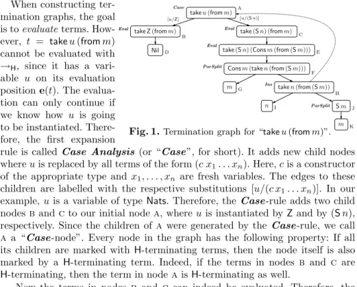
Fig. 1.Termination graph for “takeu(fromm)”. k
When constructing ter- mination graphs, the goal is toevaluateterms. How- ever, t = takeu(fromm) cannot be evaluated with
→H, since it has a vari- able u on its evaluation positione(t). The evalua- tion can only continue if we know how u is going to be instantiated. There- fore, the first expansion
rule is calledCase Analysis (or “Case”, for short). It adds new child nodes whereuis replaced by all terms of the form (c x1. . . xn). Here,cis a constructor of the appropriate type and x1, . . . , xn are fresh variables. The edges to these children are labelled with the respective substitutions [u/(c x1. . . xn)]. In our example,uis a variable of type Nats. Therefore, theCase-rule adds two child nodesbandcto our initial nodea, whereuis instantiated byZand by (Sn), respectively. Since the children of a were generated by the Case-rule, we call a a “Case-node”. Every node in the graph has the following property: If all its children are marked with H-terminating terms, then the node itself is also marked by a H-terminating term. Indeed, if the terms in nodes b and c are H-terminating, then the term in nodea isH-terminating as well.
Now the terms in nodes b and c can indeed be evaluated. Therefore, the Evaluation-rule (“Eval”) adds the nodesdanderesulting from one evaluation step with→H. Moreover,eis also anEval-node, since its term can be evaluated further to the term in node f. So the Case- andEval-rule perform a form of narrowing that respects the evaluation strategy and the types ofHaskell.
The termNilin noded cannot be evaluated and therefore,dis a leaf of the termination graph. But the term “Consm(taken(from(Sm)))” in node f may be evaluated further. Whenever the head of a term is a constructor like Cons or a variable,4then evaluations can only take place on its arguments. We use a Parameter Split-rule (“ParSplit”) which adds new child nodes with the argu- ments of such terms. Thus, we obtain the nodesgandh. Again,H-termination of the terms ingandhobviously impliesH-termination of the term in node f.
The nodegremains a leaf since its termm cannot be evaluated further for any normal ground instantiation. For nodeh, we could continue by applying the rules Case, Eval, and ParSplit as before. However, in order to obtain finite graphs (instead of infinite trees), we also have anInstantiation-rule (“Ins”).
Since the term in node h is an instance of the term in node a, one can draw aninstantiation edge from the instantiated term to the more general term (i.e., fromhtoa). We depict instantiation edges by dashed lines. These are the only edges which may point to already existing nodes (i.e., one obtains a tree if one removes the instantiation edges from a termination graph).
4 The reason is that “x t1. . . tn”H-terminates iff the termst1, . . . , tn H-terminate.
To guarantee that the term in nodehisH-terminating whenever the terms in its child nodes areH-terminating, theIns-rule has to ensure that one only uses instantiations withH-terminating terms. In our example, the variablesuandm of node aare instantiated with the terms nand (Sm), respectively. Therefore, in addition to the child a, the node h gets two more children iand j marked withnand (Sm). Finally, theParSplit-rule addsj’s childk, marked withm.
Now we consider a different start term, viz. “take”. If a defined function has
“too few” arguments, then by Def. 3 we have to apply it to additional H-ter- minating arguments in order to examine H-termination. Therefore, we have a Variable Expansion-rule (“VarExp”) which would add a child marked with
“takex” for a fresh variablex. Another application ofVarExpgives “takexxs”.
The remaining termination graph is constructed by the rules discussed before.
Definition 4 (Termination Graph). Let G be a graph with a leaf marked with the term t. We say that Gcan be expandedtoG′ (denoted “G⇒G′”) if G′ results fromGby adding newchild nodes marked with the elements ofch(t) and by adding edges from t to each element of ch(t). Only in the Ins-rule, we also permit to add an edge to an already existing node, which may then lead to cycles. All edges are marked by the identity substitution unless stated otherwise.
Eval: ch(t) ={˜t}, ift= (f t1. . . tn),f is a defined symbol,n≥arity(f),t→H˜t Case: ch(t) ={tσ1, . . . , tσk}, ift= (f t1. . . tn),f is a defined function symbol, n≥arity(f),t|e(t)is a variablexof type “d τ1...τm” for a type constructord, the type constructord has the data constructors ci of arity ni (where 1 ≤ i ≤ k), and σi = [x/(cix1. . . xni)] for fresh pairwise different variables x1, . . . , xni. The edge from t totσi is marked with the substitutionσi. VarExp: ch(t) = {t x}, if t = (f t1. . . tn), f is a defined function symbol,
n <arity(f),xis a fresh variable
ParSplit:ch(t) ={t1, ..., tn}ift= (c t1...tn),cis a constructor or variable,n >0 Ins: ch(t) ={s1, . . . , sm,˜t}, ift= (f t1. . . tn),tis not an error term,f is a de- fined symbol,n≥arity(f),t= ˜tσfor some termt,˜ σ= [x1/s1, . . . , xm/sm].
Moreover, either˜t= (x y)for fresh variablesxandy, or˜t is anEval-node, or˜tis a Case-node and all paths starting in ˜treach anEval-node or a leaf with an error term after traversing onlyCase-nodes.5 The edge from t to˜t is called an instantiation edge.
If the graph already contained a node marked witht, then we permit to re-˜ use this node in theIns-rule. So in this case, instead of adding a new child marked with˜t, one may add an edge fromt to the already existing nodet.˜ Let Gt be the graph with a single node marked with t and no edges. G is a termination graphfor t iffGt⇒∗GandGis in normal form w.r.t. ⇒.
If one disregardsIns, then for each leaf there is at most one rule applicable.6 However, theIns-rule introduces indeterminism. Instead of applying theCase- rule on nodeain Fig. 1, we could also applyIns and generate an instantiation
5 This ensures that every cycle of the graph contains at least oneEval-node.
6 No rule is applicable to leaves with variables, constructors, or error terms.
edge to a new node with ˜t= (takeuys). Since the instantiation is [ys/(fromm)], nodea would get an additional child node marked with the non-H-terminating term (fromm). Then our approach in Sect. 4 which tries to proveH-termination ofallterms in the termination graph would fail, whereas it succeeds for the graph in Fig. 1. Therefore, in our implementation we developed a heuristic for construc- ting termination graphs which tries to avoid unnecessary applications of Ins (since applyingIns means that one has to proveH-termination of more terms).
An instantiation edge to ˜t = (x y) is needed to get termination graphs for functions liketmawhich are applied to “toomany”arguments in recursive calls.
tma(Sm) =tmam m (2)
Here,tma has the typeNats →a. We obtain the termination graph in Fig. 2.
After applyingCase andEval, we result in “tmam m” in noded which is not an instance of the start term “tman” in nodea. Of course, we could continue with
tman
tma Z tma(Sm)
tmam m
tmam m
m
[n/Z] [n/(Sm)]
x y y a
Case
b c
Eval
d
Ins
f
Ins
g i
e
ParSplit
h
Fig. 2.Termination graph for “tman”
Case andEvalinfinitely often, but to obtain a termination graph, at some point we need to apply the Ins-rule.
Here, the only possibility is to regard t = (tmam m) as an instance of the term ˜t= (x y). Thus, we obtain an ins- tantiation edge to the new nodee. As the instantiation is [x/(tmam), y/m], we get additional child nodesfandg
marked with “tmam” andm, respectively. Now we can “close” the graph, since
“tmam” is an instance of the start term “tman” in nodea. So the instantiation edge to the special term (x y) is used to remove “superfluous” arguments (i.e., it permits to go from “tmam m” in nodedto “tmam” in node f). Thm. 5 shows that by the expansion rules of Def. 4 one can always obtain normal forms.7 Theorem 5 (Existence of Termination Graphs). The relation ⇒ is nor- malizing, i.e., for any termt there exists a termination graph.
4 From Termination Graphs to DP Problems
Now we present a method to proveH-termination of all terms in a termination graph. To this end, we want to use existing techniques for termination analysis of term rewriting. One of the most popular techniques for TRSs is thedependency pair (DP) method [2]. In particular, the DP method can be formulated as a gen- eral framework which permits the integration and combination of any termina- tion technique for TRSs [7]. ThisDP framework operates on so-calledDP prob- lems (P,R). Here, P and Rare TRSs that may also have rulesℓ→rwhere r contains extra variables not occurring inℓ.P’s rules are calleddependency pairs.
The goal of the DP framework is to show that there is no infinitechain, i.e., no
7 All proofs can be found in the appendix.
infinite reductions1σ1→P t1σ1 →∗R s2σ2 →P t2σ2 →∗R . . . where si →ti ∈ P andσiare substitutions. In this case, the DP problem (P,R) is calledfinite. See [7] for an overview on techniques to prove finiteness of DP problems.8
Instead of transforming termination graphs into TRSs, the information avail- able in the termination graph can be better exploited if one transforms these graphs into DP problems, cf. the end of this section. In this way, we also do not have to impose any restrictions on the form of the termination graph (as in [12] where one can only analyze certain start terms which lead to termina- tion graphs “without crossings”). Then finiteness of the resulting DP problems impliesH-termination of all terms in the termination graph.
Note that termination graphs still contain higher-order terms (e.g., applica- tions of variables to other terms like “x y” and partial applications like “takeu”).
Since most methods and tools for automated termination analysis only operate on first-order TRSs, we translate higher-order terms intoapplicative first-order terms containing just variables, constants, and a binary symbolapfor function application. So terms like “x y”, “takeu”, and “takeuxs” are transformed into the first-order termsap(x, y),ap(take, u), andap(ap(take, u),xs), respectively. As shown in [8], the DP framework is well suited to prove termination of applicative TRSs automatically. To ease readability, in the remainder we will not distinguish anymore between higher-order and corresponding applicative first-order terms, since the conversion between these two representations is obvious.
Recall that if a node in the termination graph is marked with a non-H- terminating term, then one of its children is also marked with a non-H-termina- ting term. Hence, every non-H-terminating term corresponds to an infinite path in the termination graph. Since a termination graph only has finitely many nodes, infinite paths have to end in a cycle. Thus, it suffices to proveH-termination for all terms occurring in cycles resp. in strongly connected components (SCCs) of the termination graph. Moreover, one can analyzeH-termination separately for each SCC. Here, an SCC is a maximal subgraph G′ of the termination graph such that for all nodesn1andn2inG′ there is a non-empty path fromn1ton2
traversing only nodes ofG′. (In particular, there must also be a non-empty path from every node to itself inG′.) The termination graph for “takeu(fromm)” in Fig. 1 has just one SCC with the nodesa,c,e,f,h. The following definition is needed to extract dependency pairs from SCCs of the termination graph.
Definition 6 (DP Path).LetG′ be an SCC of a termination graph containing a path from a node marked withsto a node marked witht. We say that this path is a DP pathif it does not traverse instantiation edges, if s has an incoming instantiation edge inG′, and if t has an outgoing instantiation edge in G′.
So in Fig. 1, the only DP path isa,c,e,f, h. Since every infinite path has to traverse instantiation edges infinitely often, it also has to traverse DP paths
8 In the DP literature, one usually does not regard rules with extra variables on right- hand sides, but almost all existing termination techniques for DPs can also be used for such rules. (For example, finiteness of such DP problems can often be proved by eliminating the extra variables by suitableargument filterings[2].)
infinitely often. Therefore, we generate a dependency pair for each DP path. If there is no infinite chain with these dependency pairs, then no term corresponds to an infinite path, i.e., then all terms in the graph areH-terminating.
More precisely, whenever there is a DP path from a node marked withsto a node marked withtand the edges of the path are marked withσ1, . . . , σm, then we generate the dependency pair sσ1. . . σm→t. In Fig. 1, the first edge of the DP path is labelled with the substitution [u/(Sn)] and all remaining edges are labelled with the identity. Thus, we generate the dependency pair
take(Sn) (fromm)→taken(from(Sm)). (3) The resulting DP problem is (P,R) whereP ={(3)}and R=∅.9Automated termination tools can easily show that this DP problem is finite. Hence, the start term “takeu(fromm)” isH-terminating in the originalHaskell-program.
Similarly, finiteness of the DP problem ({tma(Sm) → tmam},∅) for the start term “tman” from Fig. 2 is also easy to prove automatically.
A slightly more challenging example is obtained by replacing the lasttake- rule by the following two rules, wherepcomputes thepredecesor function.
take(Sn) (Consxxs) =Consx(take(p(Sn))xs) p(Sx) =x (4)
Consm(take(p(Sn)) (from(Sm))) toa m take(p(Sn)) (from(Sm))
p(Sn) Sm
n m
f
ParSplit
g h
Ins
i
Eval
ParSplit j
k l
Fig. 3.Subtree at nodefof Fig. 1 Now the resulting termination graph can
be obtained from the graph in Fig. 1 by replacing the subgraph starting with node fby the subgraph in Fig. 3.
We want to construct an infinite chain whenever the termination graph contains a non-H-terminating term. In this case,
there also exists a DP path with first nodessuch thatsis notH-terminating. So there is a normal ground substitution σ where sσ is not H-terminating either.
There must be a DP path from s to a term t labelled with the substitutions σ1, . . . , σm such that σis an instance of σ1. . . σm and such thattσ is also not H-terminating. So the first step of the desired corresponding infinite chain is sσ →P tσ. The node t has an outgoing instantiation edge to a node ˜t which starts another DP path. So to continue the construction of the infinite chain in the same way, we now need a non-H-terminating instantiation of ˜t with a nor- mal ground substitution. Obviously, ˜t matchest by some matcherτ. But while
˜tτ σis notH-terminating, the substitutionτ σis not necessarily a normal ground substitution. The reason is thatt and henceτ may contain defined symbols.
This is also the case in our example. The only DP path is a, c, e, f, h which would result in the dependency pair take(Sn) (fromm) → t with t = take(p(Sn)) (from(Sm)). Nowt has an instantiation edge to node a with ˜t = takeu(fromm). The matcher isτ= [u/(p(Sn)), m/(Sm)]. Soτ(u) is not normal.
In this example, the problem can be avoided by already evaluating the right- hand sides of dependency pairs as much as possible. So instead of a dependency
9 Def. 11 will explain how to generateRin general.
pair sσ1. . . σm → t we now generate the dependency pair sσ1. . . σm → ev(t).
For a node marked with t, ev(t) is the term reachable from t by traversing only Eval-nodes. So in our example ev(p(Sn)) =n, since node iis an Eval- node with an edge to node k. Moreover,ev(t) can also evaluate subterms of t ift is aParSplit-node with a constructor as head or anIns-node without an instantiation edge to the special node “x y”. We obtainev(Sm) =Smfor node j andev(take(p(Sn)) (from(Sm))) =taken(from(Sm)) for nodeh. Thus, the resulting DP problem is again (P,R) withP ={(3)}andR=∅.
To see how ev(t) must be defined for ParSplit-nodes where head(t) is a variable, we regard the functionnontermagain, cf. (1). In the termination graph for the start term “nontermb x”, we obtain a DP path from the node with the start term to a node with “nonterm(xTrue)x” labelled with the substi- tution [b/False]. So the resulting DP problem only contains the dependency pair
“nonterm Falsex → ev(nonterm(xTrue)x)”. If we would define ev(xTrue) = xTrue, thenev would not modify the term “nonterm(xTrue)x”. But then the resulting DP problem would be finite and one could falsely proveH-termination.
(The reason is that the DP problem contains no rule to transform any instance of “xTrue” toFalse.) But as discussed in Sect. 3, xcan be instantiated by ar- bitrary H-terminating functions and then, “xTrue” can evaluate to any term.
Therefore,evmust replace terms like “xTrue” by fresh variables. Similarly, ift is anIns-node with an instantiation edge to the node “x y”, then we also define ev(t) to be a fresh variable. The reason for this will become clear in the sequel, cf. Footnote 11.
Definition 7 (ev).Let Gbe a termination graph with a node t.10 Then
ev(t) = 8
>>
>>
>>
>>
>>
<
>>
>>
>>
>>
>>
:
t, iftis a leaf, aCase-node, or aVarExp-node x, for a fresh variablexif either
tis a ParSplit-node where head(t) is a variable or tis an Ins-node with an instantiation edge to “x y”
ev(˜t), iftis anEval-node with childt˜
˜t[x1/ev(t1), . . . , xn/ev(tn)], ift= ˜t[x1/t1, . . . , xn/tn]and either tis an Ins-node with the childrent1, . . . , tn,˜tor
tis a ParSplit-node, and ˜t= (c x1. . . xn) for a constructorc Our goal was to construct an infinite chain wheneversis the first node in a DP path and sσ is notH-terminating for a normal ground substitution σ. As discussed before, there is a DP path fromsto tsuch that the chain starts with sσ→P ev(t)σand such thattσand henceev(t)σis also notH-terminating. The node t has an instantiation edge to some node ˜t. Thus t = ˜t[x1/t1, . . . , xn/tn] and ev(t) = ˜t[x1/ev(t1), . . . , xn/ev(tn)]. In order to continue the construc- tion of the infinite chain, we need a non-H-terminating instantiation of ˜t with a normal ground substitution. Clearly, if ˜t is instantiated by the substitution [x1/ev(t1)σ, . . . , xn/ev(tn)σ], then it is again not H-terminating. However, the substitution [x1/ev(t1)σ, . . . , xn/ev(tn)σ] is not necessarily normal. The prob- lem is that ev does not perform those evaluations that correspond to instan-
10To simplify the presentation, we identify nodes with the terms they are labelled with.
tiation edges and to edges from Case-nodes. Therefore, we now generate DP problems which do not just contain dependency pairs P, but they also contain all rulesRwhich might be needed to evaluateev(ti)σfurther. Then we obtain sσ→P ev(t)σ→∗Rtσ˜ ′ for a normal ground substitutionσ′. Since ˜tis again the first node in a DP path, now this construction of the chain can be continued in the same way infinitely many times. Hence, we obtain an infinite chain.
p(Sn)
p(S Z) p(S(Sx))
Z S(p(Sx))
p(Sx) x
[n/Z] [n/(Sx)]
Case i
m
Eval
n
Eval
o p
ParSplit
q
Ins
r
Fig. 4.Subtree at nodeiof Fig. 3
As an example, we replace the equation for pin (4) by the following two defining equations:
p(S Z) =Z p(Sx) =S(px) (5) In the termination graph for “takeu(fromm)”
from Fig. 1 and 3, the node i would now be replaced by the subtree in Fig. 4. So iis now a Case-node. Thus, instead of (3) we obtain the dependency pair
take(Sn) (fromm)→take(p(Sn)) (from(Sm)), (6) since now ev does not modify its right-hand side anymore (i.e., ev(p(Sn)) = p(Sn)). Hence, now the resulting DP problem must contain all rules R that might be used to evaluatep(Sn) when instantiated byσ.
So for any term t, we want to detect rules that might be needed to eval- uate ev(t)σ further for normal ground substitutions σ. To this end, we first compute the set con(t) of those terms that are reachable from t, but where the computation of evstopped. Socon(t) contains all terms which might give rise to furthercontinuing evaluations that are not captured byev. To compute con(t), we traverse all paths starting in t. If we reach aCase-nodes, we stop traversing this path and insert s into con(t). Moreover, if we traverse an in- stantiation edge to some node ˜t, we also stop and insert ˜t into con(t). So in the example of Fig. 4, we obtaincon(p(Sn)) ={p(Sn)}, sinceiis now aCase- node. If we started with the termt=take(Sn) (fromm) in nodec, then we would reach the Case-node iand the node a which is reachable via an instantiation edge. Socon(t) ={p(Sn),takeu(fromm)}. Finally,conalso stops atVarExp- nodes (they are in normal form w.r.t. →H), atParSplit-nodes whose head is a variable and atIns-nodes with an instantiation edge to “x y” (sinceevalready
“approximates” their result by fresh variables).11
11 The special treatment of Ins-nodes t=t1t2 with an instantiation edge to “x y”
was not considered in the definitions ofevandconin [9]. If they were handled like ordinaryIns-nodes, then we would obtainev(t) =ev(t1)ev(t2). But thencon(t1) and con(t2) could be empty although “ev(t1)σev(t2)σ” can be evaluated further for a normal ground substitutionσ.
As an example, consider the termination graph resulting from the non-terminating program with the defining equations “f Zz=f(idzZ)z” and “idx=x”.
Definition 8 (con). Let Gbe a termination graph with a node t. Then
con(t) = 8
>>
>>
>>
<
>>
>>
>>
:
∅, iftis a leaf, aVarExp-node, a ParSplit-node with variable head, or an Ins-node with instantiation edge to “x y”
{t}, iftis a Case-node
{˜t} ∪con(t1)∪. . .∪con(tn), iftis an Ins-node with the children t1, . . . , tn,˜tand an instantiation edge fromtto˜t S
t′child oftcon(t′), otherwise
Now we can define how to extract a DP problem dpG′ from every SCC G′ of the termination graph. As mentioned, we generate a dependency pair sσ1. . . σm→ev(t) for every DP path fromstotlabelled withσ1, . . . , σminG′. If t= ˜t[x1/t1, . . . , xn/tn] has an instantiation edge to ˜t, then the resulting DP problem must contain all rules that can be used reduce the terms in con(t1)∪ . . .∪con(tn). For any terms, letrl(s) be the rules that can be used to reducesσ for normal ground substitutionsσ. We will give the definition ofrlafterwards.
Definition 9 (dp). For a termination graph containing an SCC G′, we define dpG′= (P,R). Here,P andRare the smallest sets such that
• “sσ1. . . σm→ev(t)” ∈ P and
• rl(q)⊆ R,
wheneverG′ contains a DP path fromstotlabelled withσ1, . . . , σm,t= ˜t[x1/t1, . . . , xn/tn] has an instantiation edge to˜t, andq∈con(t1)∪. . .∪con(tn).
In our example with the start term “takeu(fromm)” and the p-equations from (5), the termination graph in Fig. 1, 3, and 4 has two SCCsG1(consisting of the nodesa,c,e,f,h) andG2(consisting ofi,n,p,q). Finiteness of the two DP problemsdpG1anddpG2can be proved independently. The SCCG1only has the DP path fromatohleading to the dependency pair (6). So we obtaindpG1= ({(6)},R1) whereR1 contains rl(q) for all q∈con(p(Sn)) ={p(Sn)}. Thus, R1=rl(p(Sn)). The SCCG2only has the DP path fromitoq. Hence,dpG2= (P2,R2) whereP2 consists of the dependency pair “p(S(Sx))→p(Sx)” (since ev(p(Sx)) =p(Sx)) andR2containsrl(q) for allq∈con(x) =∅, i.e.,R2=∅. Thus, finiteness ofdpG2 can easily be proved automatically.
For every term s, we now show how to extract a set of rules rl(s) such that every evaluation ofsσ for a normal ground substitution σ corresponds to
fx z f Zz f(idzZ)z
idzZ x y
idz Z y
z
[x/Z] Case
Eval
Ins
Ins ParSplit
Eval
From the DP path, we obtain the dependency pair
“f Z z →ev(f (id z Z) z)”, where ev(f (id z Z) z) = f ev(id z Z)z. With our current definition,ev(idz Z) is a fresh variable and therefore, the dependency pair is
“f Zz→fx z” which gives rise to an infinite chain.
But if we treated “id zZ” as an ordinaryIns-node, we would get ev(id z Z) =ev(id z)ev(Z) =z Z and the dependency pair would be “f Z z → f (z Z) z”.
The resulting DP problem would contain no rules, since con(idz)∪con(Z) =∅. So then we could falsely prove H-termination off.
a reduction with rl(s).12 The only expansion rules which transform terms into
“equal” ones areEval andCase. This leads to the following definition.
Definition 10 (Rule Path). A path from a node marked with s to a node marked with t is a rule path if s and all other nodes on the path except t are Eval- or Case-nodes andtis no Eval- or Case-node. Sotmay also be a leaf.
In Fig. 4, there are two rule paths starting in nodei. The first one isi,m,o (since ois a leaf) and the other isi,n,p(since pis aParSplit-node).
While DP paths give rise to dependency pairs, rule paths give rise to rules.
Therefore, if there is a rule path fromstotlabelled withσ1, . . . , σm, thenrl(s) contains the rule sσ1. . . σm → ev(t). In addition, rl(s) must also contain all rules required to evaluateev(t) further, i.e., all rules inrl(q) forq∈con(t).13 Definition 11 (rl). For a node labelled withs,rl(s)is the smallest set with
• “sσ1. . . σm→ev(t)” ∈rl(s)and
• rl(q)⊆rl(s),
whenever there is rule path fromstotlabelled withσ1, . . . , σm, andq∈con(t).
For the start term “takeu(fromm)” and the p-equations from (5), we ob- tained the DP problemdpG1= ({6},rl(p(Sn))). Here, rl(p(Sn)) consists of
p(S Z)→Z (due to the rule path fromito o) (7) p(S(Sx))→S(p(Sx)) (due to the rule path fromitop), (8) asevdoes not modify the right-hand sides of (7) and (8). Moreover, the require- ment “rl(q)⊆rl(p(Sn)) for allq∈con(Z) and allq∈con(S(p(Sx)))” does not add further rules. The reason is thatcon(Z) =∅andcon(S(p(Sx))) ={p(Sn)}.
Now finiteness ofdpG1 = ({6},{(7),(8)}) is also easy to show automatically.
Finally, consider the following program which leads to the graph in Fig. 5.
fx=applyToZero f applyToZerox=xZ
This example shows that one also has to traverse edges resulting fromVarExp when constructing dependency pairs. Otherwise one would falsely proveH-termi- nation. Since the only DP path goes from nodeatof, we obtain the DP problem ({fx→fy},R) withR=rl(y) =∅. This problem is not finite (and indeed, “fx”
is notH-terminating). In contrast, the definition of rlstops atVarExp-nodes.
12More precisely, sσ →∗H q implies sσ →∗rl(s) q′ for a term q′ which is “at least as evaluated” asq (i.e., one can evaluateqfurther toq′if one also permits evaluation steps below or beside the evaluation position).
13So ift= ˜t[x1/t1, . . . , xn/tn] has an instantiation edge to ˜t, then here we also include all rules ofrl(˜t), sincecon(t) ={˜t} ∪con(t1)∪. . .∪con(tn). In contrast, for the definition ofdpin Def. 9 we only regard the rulesrl(q) forq∈con(t1)∪. . .∪con(tn), whereas the evaluations of ˜tare captured by the dependency pairs.
fx
applyToZero f applyToZerox
f xZ
fy Z
y a
Eval
b
Ins
c
Eval
d
VarExp
e
ParSplit
Ins
f g
h
Fig. 5.Termination graph for “fx”
The example also illustrates thatrl and dp handle instantiation edges differently, cf. Foot- note 13. Since there is a rule path fromatob, we would obtain rl(fx) = {fx→applyToZero f} ∪ rl(applyToZerox), since con(applyToZero f) = applyToZerox. So for the construction of rl we also have to include the rules resulting from nodes likecwhich are only reachable by instan- tiation edges.14 We obtainrl(applyToZerox) =
{applyToZerox → z}, since ev(xZ) = z for a fresh variable z. The following theorem states the soundness of our approach.
Theorem 12 (Soundness). Let G be termination graph. If the DP problem dpG′ is finite for all SCCsG′ of G, then all nodes t inGare H-terminating.15
While we transform termination graphs into DP problems, it would also be possible to transform termination graphs into TRSs instead and then prove ter- mination of the resulting TRSs. However, this approach has several disadvanta- ges. For example, if the termination graph contains a VarExp-node or aPar- Split-node with a variable as head, then we would result in rules with extra va- riables on right-hand sides and thus, the resulting TRSs would never be termi- nating. In contrast, a DP problem (P,R) with extra variables in P andRcan still be finite, since dependency pairs from P are only applied on top positions in chains and since Rneed not be terminating for finite DP problems (P,R).
5 Extensions, Implementation, and Experiments
We presented a technique for automated termination analysis of Haskell which works in three steps: First, it generates a termination graph for the given start term. Then it extracts DP problems from the termination graph. Finally, one uses existing methods from term rewriting to prove finiteness of these DP problems.
To ease readability, we did not regardHaskell’stype classes and built-in data structures in the preceding sections. However, our approach easily extends to these concepts [15]. To deal with type classes, we use an additionalCase-rule in the construction of termination graphs, which instantiates type variables by all instances of the corresponding type class. Built-in data structures like Haskell’s lists and tuples simply correspond to user-defined types with a different syntax.
To deal with integers, we transform them into a notation with the constructors PosandNeg(which take arguments of typeNats) and provide pre-defined rewrite rules for integer operations like addition, subtraction, etc. Floating-point num- bers can be handled in a similar way (e.g., by representing them as fractions).
14This is different in the definition ofdp. Otherwise, we would haveR=rl(y)∪rl(fx).
15Instead ofdpG′ = (P,R), forH-termination it suffices to prove finiteness of (P♯,R).
Here,P♯results from P by replacing each rulef(t1, ..., tn)→g(s1, ..., sm) inP by f♯(t1, ..., tn)→g♯(s1, ..., sm), wheref♯andg♯are fresh “tuple” function symbols [2].
We implemented our approach in the termination proverAProVE[10]. It ac- cepts the fullHaskell 98language defined in [13] and we successfully evaluated our implementation with standardHaskell-libraries from theHugs-distribution such asPrelude,Monad,List,FiniteMap, etc. To access the implementation via a web interface and for details on our experiments see http://aprove.informatik.
rwth-aachen.de/eval/Haskell/.
We conjecture that term rewriting techniques are also suitable for termination analysis of other kinds of programming languages. In [14], we recently adapted the dependency pair method in order to prove termination oflogicprogramming languages like Prolog. In future work, we intend to examine the use of TRS- techniques forimperative programming languages as well.
References
1. A. Abel. Termination checking with types. RAIRO - Theoretical Informatics and Applications, 38(4):277–319, 2004.
2. T. Arts and J. Giesl. Termination of term rewriting using dependency pairs. The- oretical Computer Science, 236:133–178, 2000.
3. G. Barthe, M. J. Frade, E. Gim´enez, L. Pinto, and T. Uustalu. Type-based termi- nation of recursive definitions. Math. Structures in Comp. Sc., 14(1):1–45, 2004.
4. O. Fissore, I. Gnaedig, and H. Kirchner. Outermost ground termination. InProc.
WRLA ’02, ENTCS 71, 2002.
5. J. Giesl. Termination analysis for functional programs using term orderings. In Proc. SAS’ 95, LNCS 983, pages 154–171, 1995.
6. J. Giesl and A. Middeldorp. Transformation techniques for context-sensitive rewrite systems. Journal of Functional Programming, 14(4):379–427, 2004.
7. J. Giesl, R. Thiemann, and P. Schneider-Kamp. The dependency pair framework:
Combining techniques for automated termination proofs. InProc. LPAR ’04, LNAI 3452, pages 301–331, 2005.
8. J. Giesl, R. Thiemann, and P. Schneider-Kamp. Proving and disproving termina- tion of higher-order functions. InProc. FroCoS ’05, LNAI 3717, pp. 216-231, 2005.
9. J. Giesl, S. Swiderski, P. Schneider-Kamp, and R. Thiemann. Automated Termi- nation Analysis forHaskell: From Term Rewriting to Programming Languages. In Proc. RTA ’06, LNCS, 2006. To appear.
10. J. Giesl, P. Schneider-Kamp, and R. Thiemann. AProVE 1.2: Automatic termina- tion proofs in the DP framework. InProc. IJCAR ’06, LNAI, 2006. To appear.
11. C. S. Lee, N. D. Jones, and A. M. Ben-Amram. The size-change principle for program termination. InProc. POPL ’01, pages 81–92. ACM Press, 2001.
12. S. E. Panitz and M. Schmidt-Schauss. TEA: Automatically proving termination of programs in a non-strict higher-order functional language. In Proc. SAS ’97, LNCS 1302, pages 345–360, 1997.
13. S. Peyton Jones (ed.). Haskell 98 Languages and Libraries: The revised report.
Cambridge University Press, 2003.
14. P. Schneider-Kamp, J. Giesl, A. Serebrenik, and R. Thiemann. Automated ter- mination analysis for logic programs by term rewriting. In Proc. LOPSTR ’06, LNCS, 2006. To appear.
15. S. Swiderski. Terminierungsanalyse von Haskellprogrammen. Diploma Thesis, RWTH Aachen, 2005. Seehttp://aprove.informatik.rwth-aachen.de/eval/Haskell/.
16. A. Telford and D. Turner. Ensuring termination in ESFP. Journal of Universal Computer Science, 6(4):474–488, 2000.
17. C. Walther. On proving the termination of algorithms by machine. Artificial Intelligence, 71(1):101–157, 1994.
18. H. Xi. Dependent types for program termination verification. Higher-Order and Symbolic Computation, 15(1):91–131, 2002.
A Proofs
Theorem 5 (Existence of Termination Graphs). The relation ⇒ is nor- malizing, i.e., for any termt, there exists a termination graph.
Proof. We first construct a graph G in normal form w.r.t. ⇒ which contains nodes marked with “f x1. . . xn” for all defined symbolsf where thexi are pair- wise fresh variables and arity(f) =n. Then, by performing suitable expansion steps and by adding instantiation edges to these nodes, the graphGt(which only consists of one node which is marked with t) can be transformed into normal form. Here, in the end all nodes which are not reachable fromtare removed.
To constructG, we start with the nodes “f x1. . . xn” for all defined symbols f. Currently, these nodes are not reached by any edges. By performing Case- and Eval-steps, we obtain paths from “f x1. . . xn” to all right-hand sides of f-rules. Then we apply the following procedure: We apply ParSplit until we end up with leaves of the form “g s1. . . sk” for defined symbolsg. Ifk= arity(g), then we can add an instantiation edge to the already existing node “g x1. . . xk” and continue this process with the nodes s1, . . . , sk (i.e., we apply ParSplit again until we reach leaves with a defined symbol as head). If k < arity(g), then we perform a number ofVarExp-steps to obtain a term where the number of arguments of g is arity(g). If k > arity(g), then we perform Ins-steps with instantiation edges to the node “x y” until we obtain a term where the number
of arguments ofg is arity(g). ⊓⊔
To prove the soundness theorem of our approach (Thm. 12), we need a lemma about the semantics of ev, con, and rl (Lemma 18) and a lemma about the semantics ofdp (Lemma 20). To describe the semantics ofev,con, andrl, we use the following relation⇒H, which also permits reductions on positions beside or below the evaluation position.
Definition 13 (⇒H). We havet⇒Hsifft rewrites toson a positionπwhich is not strictly abovee(t) using the first equation of the program whose left-hand side matchest|π.
The following lemma shows that⇒Hallows us to simulate all reductions that are performed by the function ev.
Lemma 14 (Simulation of ev by ⇒H). Let G be a termination graph and letσ be a substitution. Iftσ⇒∗Hev(t)σholds for all ParSplit- and Ins-nodes t whereev(t) is a fresh variable, thentσ⇒∗Hev(t)σholds for all nodes t of the termination graph G.
Proof. We use induction on the edge-relation ofGwhere we remove all instanti- ation edges. This relation is well founded, since after the removal of the instan- tiation edges, Gis an acyclic graph. We only have to consider the cases where ev(t)6=t and whereev(t) is not a fresh variable.
Iftis anEval-node with child ˜t, then we havetσ→H˜tσand thus,tσ⇒Htσ.˜ By the induction hypothesis we obtain ˜tσ ⇒∗Hev(˜t)σ and hencetσ ⇒H˜tσ⇒∗H
ev(˜t)σ=ev(t)σ.
Ift = (c t1. . . tn) is a ParSplit-node with a constructor as head, then we directly obtain the result from the induction hypotheses for the childrenti:
tσ= (c t1σ . . . tnσ)⇒∗H(cev(t1)σ . . .ev(tn)σ) =ev(t)σ
Finally, ift= ˜t[x1/t1, . . . , xn/tn] is anIns-node with an instantiation edge to an Eval- or Case-node ˜t, then we proceed in a similar way by using the induction hypotheses for theti:
tσ = ˜t[x1/t1, . . . , xn/tn]σ
= ˜tσ[x1/t1σ, . . . , xn/tnσ]
⇒∗H˜tσ[x1/ev(t1)σ, . . . , xn/ev(tn)σ]
= ˜t[x1/ev(t1), . . . , xn/ev(tn)]σ
= ev(t)σ
⊓
⊔ Lemma 18 about the semantics ofev,con, and rlshows a kind of converse to Lemma 14, i.e., how to simulate reductions with →H by ev, con, and rl.
Essentially, our goal is to show that ift is a node in the termination graph and there is a reduction tσ →∗H q, then we also have ev(t)σ →∗S
s∈con(t)rl(s) q′ for some termq′ withq⇒∗Hq′.
Since the rules S
s∈con(t)rl(s) do not take σ into account, this does not hold in general if the terms introduced by σ are evaluated in the reduction tσ →∗H q. A possibility would be to restrict ourselves to normal substitutions σ, i.e., to substitutions whereσ(x) is in normal form w.r.t.→Hfor all variables x. However, to ease the proof of Lemma 18, we consider a slightly larger class of substitutions. We only require that σ is evaluated enough in the reduction tσ →∗H q. This means that in this reduction we do not evaluate those terms introduced byσwhich may have a non-functional type. (Terms with functional type may lead to future evaluations when supplied with an argument. However, this does not lead to any problems for our desired lemma, because evreplaces such subterms by fresh variables.)
We formalize this concept in the two following definitions. Here, drop replaces all non-functional terms by fresh variables, except those terms whose head is already a constructor.
Definition 15 (drop,undrop). We define a functiondropfrom terms to terms as follows:
– drop(t) =t, ift has a functional type (i.e., an instance of the type a→b) – drop(c t1. . . tn) =cdrop(t1). . .drop(tn), if c is a constructor of arityn – drop(t) =xt, otherwise; herextis some fresh variable
We defineundropas the inverse function ofdrop, i.e.,undropis the substitution which replaces every variable xt by t. For any substitution σ, let σdrop be the substitution with σdrop(x) = drop(σ(x)) for all variables x. (Here, we allow substitutions with infinite domains.)
For example, if we have a data type
data Da= C(a→a) |Ea |Ga a
and a defined functionfof typea, then we obtain drop(f) =xf, drop(E f) =Exf, drop(C f) =C f(since here, the subterm f has typea→a), and drop(G f) =G f (since here, “G f” has the functional typea→Da).
Now we define that a substitution is evaluated enough for a reduction if this reduction could also be performed when replacing all terms introduced by the substitution (except constructors and terms of functional type) by fresh variables. The constructors cannot be replaced since they are needed for pattern matching. The terms of functional types cannot be replaced either since they can be substituted for variables in the heads of subterms (i.e., for variables x in subterms of the form “x t1. . . tn” and they can be further evaluated when supplied with suitable argumentst1. . . tn).
Definition 16 (Evaluated Enough). We say that a substitution σ is eval- uated enough in a (possibly infinite) reduction tσ →H t1 →H t2 →H . . . iff tσdrop→Hs1→Hs2→H. . . andti= undrop(si) for alli.
An evaluated enough substitution may introduce terms of functional type which may be evaluated further during a reduction. We have to ensure that such an evaluation only happens if this is required in order to obtain again a subterm with a constructor as head. Otherwise, tσ →∗H q does not imply ev(t)σ →∗S
s∈con(t)rl(s) q′ for some term q′ with q ⇒∗H q′. The reason is thatt could be a variablexat a leaf of the termination graph andσcould instantiate xby a term of functional type which is then reduced toq.
Therefore, we restrict ourselves to so-callednecessary reductions tσ →∗H q.
These reductions are needed in order to facilitate pattern matching. The idea of necessary reductions is the following restriction: “if one performs reductions at all, then one has to evaluate until the head is a constructor”.
Definition 17 (Necessary Reduction). We say that a reduction t →∗H s is necessaryifft=sor boths= (c s1. . . sn)for some constructorc of aritynand – t=c t1. . . tn and all reductionsti→∗Hsi are necessary or – t= (f t1. . . tk)→∗H (g l1. . . lm)→H (c r1. . . rn) for some defined symbol g
and all reductionsri→∗Hsi are necessary.
Note that whenevertstarts a necessary reduction of length greater than zero, thenthas a base type, sincetcan be reduced to (c s1. . . sn) for some constructor c of arityn.
Now we can prove the desired lemma which states the needed properties of ev,con, and rl.