Automated Termination Proofs for by Term Rewriting

(1)

Automated Termination Proofs for by Term Rewriting

J¨urgen Giesl, RWTH Aachen University, Germany Matthias Raffelsieper, TU Eindhoven, The Netherlands

Peter Schneider-Kamp, University of Southern Denmark, Odense, Denmark Stephan Swiderski, RWTH Aachen University, Germany

Ren´e Thiemann, University of Innsbruck, Austria

There are many powerful techniques for automated termination analysis of term rewriting. How- ever, up to now they have hardly been used for real programming languages. We present a new approach which permits the application of existing techniques from term rewriting to prove termination of most functions defined inHaskellprograms. In particular, we show how termination techniques for ordinary rewriting can be used to handle those features ofHaskellwhich are miss- ing in term rewriting (e.g., lazy evaluation, polymorphic types, and higher-order functions). We implemented our results in the termination proverAProVE and successfully evaluated them on existingHaskell-libraries.

Categories and Subject Descriptors: F.3.1 [Logic and Meanings of Programs]: Specifying and Verifying and Reasoning about Programs—Mechanical verification; D.1.1 [Programming Techniques]: Applicative (Functional) Programming; I.2.2 [Artificial Intelligence]: Automatic Programming—Automatic analysis of algorithms; I.2.3 [Artificial Intelligence]: Deduction and Theorem Proving

General Terms: Languages, Theory, Verification

Additional Key Words and Phrases: functional programming,Haskell, termination analysis, term rewriting, dependency pairs

Supported by the Deutsche Forschungsgsmeinschaft DFG under grant GI 274/5-2 and the DFG Research Training Group 1298 (AlgoSyn).

Authors’ addresses:

J¨urgen Giesl, Stephan Swiderski, LuFG Informatik 2, RWTH Aachen University, Ahornstr. 55, 52074 Aachen, Germany,{giesl,swiderski}@informatik.rwth-aachen.de

Matthias Raffelsieper, Dept. of Mathematics and Computer Science, TU Eindhoven, P.O. Box 513, 5600 MB Eindhoven, The Netherlands,m.raffelsieper@tue.nl

Peter Schneider-Kamp, Dept. of Mathematics and Computer Science, University of Southern Denmark, Campusvej 55, DK-5230 Odense M, Denmark,petersk@imada.sdu.dk

Ren´e Thiemann, Institute of Computer Science, University of Innsbruck, Technikerstr. 21a, 6020 Innsbruck, Austria,rene.thiemann@uibk.ac.at.

Most of the work was carried out while the authors were at the LuFG Informatik 2, RWTH Aachen University.

Permission to make digital/hard copy of all or part of this material without fee for personal or classroom use provided that the copies are not made or distributed for profit or commercial advantage, the ACM copyright/server notice, the title of the publication, and its date appear, and notice is given that copying is by permission of the ACM, Inc. To copy otherwise, to republish, to post on servers, or to redistribute to lists requires prior specific permission and/or a fee.

c

2010 ACM 0164-0925/2010/0500-0001 $5.00

(2)

1. INTRODUCTION

In the area of term rewriting, techniques for automated termination analysis have been studied for decades. While early work focused on the development of suitable well-founded orders (see e.g. [Dershowitz 1987] for an overview), in the last 10 years much more powerful methods were introduced which can handle large and realistic term rewrite systems (TRSs); see e.g. [Endrullis et al. 2008; Geser et al. 2004; Hirokawa and Middeldorp 2005; Giesl et al. 2006c; Zantema 2003].

Moreover, numerous powerful automatic tools for termination analysis of TRSs have been developed whose power is demonstrated at the annual International Termination Competition. For more information on the competition, we refer to http://termination-portal.org/wiki/Termination_Competition.

However, in order to make methods for termination analysis of term rewriting applicable in practice, one has to adapt them to real existing programming languages. In this paper, we show for the first time that termination techniques from term rewriting are indeed very useful for termination analysis of functional programming languages. Specifically, we consider the languageHaskell [Peyton Jones 2003], which is one of the most popular functional programming languages.

Since term rewriting itself is a Turing-complete programming language, in principle it is of course possible to translate any program from any programming language into an equivalent TRS and then prove termination of the resulting TRS. However in general, it is not clear how to obtain an automatic translation that creates TRSs which aresuitable for existing automated termination techniques. In other words, a naive translation of programs into TRSs is likely to produce very complicated TRSs whose termination can hardly be shown by existing automated techniques and tools.

Although functional programming languages are in some sense “close” to term rewriting, the application and adaption of TRS-techniques for termination analysis ofHaskellis still challenging for several reasons:

• Haskell has a lazy evaluation strategy. However, most TRS-techniques ignore such evaluation strategies and try to prove thatall (or all innermost) reductions terminate.¹

• Defining equations inHaskell are handled from top to bottom. In contrast, for TRSs,any rule may be used for rewriting.

• Haskellhas polymorphic types, whereas TRSs are untyped.

• InHaskell-programs with infinite data objects, only certain functions are terminating. But most TRS-methods try to prove termination ofall terms.

• Haskell is a higher-order language, whereas most automatic termination techniques for TRSs only handle first-order rewriting.

There are many papers on verification of functional programs (see e.g. [Kobayashi 2009; Ong 2006; Rondon et al. 2008] for some of the most recent approaches). How- ever, up to now there exist only few techniques for automated termination analysis

1Very recently, there has been work on termination analysis of rewriting under an outermost evaluation strategy [Endrullis and Hendriks 2009; Gnaedig and Kirchner 2008; Raffelsieper and Zantema 2009; Thiemann 2009], which however does not correspond to the lazy evaluation strategy ofHaskell(as illustrated later in Section 2.2).

ACM Transactions on Programming Languages and Systems, Vol. V, No. N, November 2010.

(3)

of functional languages. Methods for first-order languages with strict evaluation strategy were for example developed in [Giesl 1995; Lee et al. 2001; Manolios and Vroon 2006; Walther 1994], where thesize-change method of [Lee et al. 2001] was also extended to the higher-order setting [Sereni and Jones 2005; Sereni 2007]. The static call graph constructed by the methods of [Sereni and Jones 2005; Sereni 2007] is related to the graphs constructed in our approach in order to analyze termination. However, the size-change method fixes one particular order to compare values for each data type. (This also holds for higher-order types whose values are closures. These closures are typically compared by the subtree order.) Here our approach is more flexible, because the orders to compare values are not fixed.

Instead, we translate all data objects (including objects of higher-order type) into first-order terms and afterwards, one can use existing techniques from term rewriting to automatically generate suitable well-founded orders comparing these terms.

For a thorough comparison of the size-change method with techniques from term rewriting, we refer to [Thiemann and Giesl 2005].

For higher-order languages, several papers study how to ensure termination by typing (e.g. [Abel 2004; Barthe et al. 2000; Blanqui 2004; Xi 2002]) and [Telford and Turner 2000] define a restricted language where all evaluations terminate. A suc- cessful approach for automated termination proofs for a smallHaskell-like language was developed in [Panitz and Schmidt-Schauß 1997] and extended and implemented in [Panitz 1997].² This approach is related to the technique of [Gnaedig and Kirch- ner 2008], which handles outermost evaluation of untyped first-order rewriting.

However, these are all “stand-alone” methods which do not allow the use of modern termination techniques from term rewriting. Indeed, the general opinion of the Haskellcommunity was that “current advances in automatic termination proofs are still limited, especially for lazy programs” [Xu et al. 2009].

In our approach we build upon the method of [Panitz and Schmidt-Schauß 1997], but we adapt it in order to make TRS-techniques applicable.³ As shown by our experimental evaluation, the coupling with modern powerful TRS-techniques solves the previous limitations of termination methods for lazy functional programs. Now automated termination proofs for functions from real Haskell-libraries indeed become feasible.

We recapitulateHaskell in Section 2 and introduce our notion of “termination”.

As described in Section 3, to analyze termination, our method first generates a cor- respondingtermination graph(similar to the “termination tableaux” in [Panitz and Schmidt-Schauß 1997]). But in contrast to [Panitz and Schmidt-Schauß 1997], then our method transforms the termination graph intodependency pair problemswhich can be handled by existing techniques from term rewriting (Section 4). Our ap-

2In addition to methods which analyze the termination behavior of programs, there are also several results on ensuring the termination of program optimization techniques like partial evaluation, e.g.

[Glenstrup and Jones 2005]. Here, in particular the approach of [Sørensen and Gl¨uck 1995] uses graphs that are similar to the termination graphs in [Panitz and Schmidt-Schauß 1997] and in our approach.

3Alternatively as discussed in [Giesl and Middeldorp 2004], one could try to simulate Haskell’s evaluation strategy bycontext-sensitive rewriting[Lucas 1998]. But in spite of recent progress in that area (e.g. [Giesl and Middeldorp 2004; Alarc´on et al. 2006; Alarc´on et al. 2008]), termination of context-sensitive rewriting is still hard to analyze automatically.

(4)

proach can deal with any termination graph, whereas [Panitz and Schmidt-Schauß 1997] can only handle termination graphs of a special form (“without crossings”).⁴ While the dependency pair problems in Section 4 still contain higher-order functions, in Section 5 we improve the construction in order to obtainfirst-order dependency pair problems. Section 6 extends our approach to handle more types of Haskell, in particular type classes. We implemented all our contributions in the termination proverAProVE[Giesl et al. 2006b]. Section 7 presents extensive experiments which show that our approach gives rise to a very powerful fully automated termination tool. More precisely, when testing it on existing standard Haskell- libraries, it turned out that AProVE can fully automatically prove termination of the vast majority of the functions in the libraries. This shows for the first time that

• it is possible to build a powerful automated termination analyzer for a functional language likeHaskelland that

• termination techniques from term rewriting can be successfully applied to real programming languages in practice.

2. HASKELL

A real programming language likeHaskelloffers many syntactical constructs which ease the formulation of programs, but which are not necessary for the expressiveness of the language. To analyze termination of aHaskell-program, it is first checked for syntactical correctness and for being well typed. To simplify the subsequent termination analysis, our termination tool then transforms the givenHaskell-program into an equivalentHaskell-program which only uses a subset of the constructs available inHaskell. We now give the syntax and semantics for this subset ofHaskell. In this subset, we only use certain easy patterns and terms (without “λ”), and we only allow function definitions without “case”-expressions or conditionals. So we only permit case analysis by pattern-matching left-hand sides of defining equations.⁵

Indeed, any Haskell-program can automatically be transformed into a program from this subset, see [Swiderski 2005]. For example, in our implementation, lambda abstractions are removed by a form of lambda lifting. More precisely, we replace ev- eryHaskell-term “\t1. . . tn→t” with the free variablesx1, . . . , xmby “fx1. . . xm”.

Here,fis a new function symbol with the defining equationfx1. . . xmt1. . . tn =t.

2.1 Syntax of Haskell

In our subset ofHaskell, we permit user-defined data types such as data Nats = Z|S Nats data Lista= Nil|Consa(Lista)

These data-declarations introduce two type constructors Nats and List of arity 0 and 1, respectively. So Nats is a type and for every type τ, “List τ” is also a

4We will illustrate the difference in more detail in Example 5.2.

5Of course, it would be possible to restrict ourselves to programs from an even smaller “core”- Haskellsubset. However, this would not simplify the subsequent termination analysis any further.

In contrast, the resulting programs would usually be less readable, which would also make it harder for the user to understand their (automatically generated) termination proofs.

(5)

type representing lists with elements of type τ. Apart from user-defined data- declarations, there are also pre-defineddata-declarations like

data Bool = False|True.

Moreover, there is a pre-defined binary type constructor→for function types. So ifτ1 and τ2 are types, then τ1 →τ2 is also a type (the type of functions from τ1

toτ2). SinceHaskell’s type system is polymorphic, it also hastype variables likea which stand for any type, and “Lista” is the type of lists where the elements can have any type a. So the set of types is the smallest set which contains all type variables and where “d τ1. . . τn” is a type wheneverdis a type constructor of arity mandτ1, . . . , τn are types with n≤m.⁶

For each type constructor likeNats, a data-declaration also introduces its data constructors (e.g.,ZandS) and the types of their arguments. Thus,Zhas arity 0 and is of typeNatsandShas arity 1 and is of typeNats→Nats.

Apart fromdata-declarations, a program has function declarations.

Example 2.1 (takeandfrom). In the following example, “fromx” generates the infinite list of numbers starting withxand “takenxs” returns the firstnelements of the list xs. The type of from is “Nats → (List Nats)” and take has the type

“Nats→(Lista)→(Lista)” whereτ1→τ2 →τ3 stands forτ1 →(τ2→τ3). Such type declarations can also be included in theHaskell-program, as shown below.

from :: Nats→(List Nats) take :: Nats→(Lista)→(Lista) fromx= Consx(from(Sx)) take Zxs =Nil

takenNil=Nil

take(Sn) (Consxxs) =Consx(takenxs) In general, the equations in function declarations have the form “f ℓ1. . . ℓn =r”

forn≥0. The function symbolsf at the “outermost” position of left-hand sides are calleddefined. So the set of function symbols is the disjoint union of the (data) constructors and the defined function symbols. All defining equations forf must have the same number of argumentsn(calledf’sarity). The right-hand sideris an arbitraryterm, whereasℓ1, . . . , ℓn are special terms, so-calledpatterns. Moreover, the left-hand side must be linear, i.e., no variable may occur more than once in

“f ℓ1. . . ℓn”.

The set of terms is the smallest set containing all variables, function symbols, and well-typed applications (t1t2) for termst1 and t2. As usual, “t1t2t3” stands for “((t1t2)t3)”, etc. The set of patterns is the smallest set with all variables and all linear terms “c t1. . . tn” where c is a constructor of arity n and t1, . . . , tn are patterns.

Thepositions of t are P os(t) ={ε} if t is a variable or function symbol. Oth- erwise, P os(t1t2) ={ε} ∪ {1π| π∈P os(t1)} ∪ {2π| π∈P os(t2)}. As usual, we define t|ε =t and (t1t2)|i π =ti|π for i ∈ {1,2}. The term q is a subterm of t, i.e. qt, if a position πof texists such that t|π =q. The head of tis t|1ⁿ where

6Moreover,Haskellalso has several built-in primitive data types (e.g.,Int,Char,Float, . . . ) and its type system also featurestype classesin order to permit overloading of functions. To ease the presentation, we ignore these concepts at the moment and refer to Section 6 for an extension of our approach to built-in data types and type classes.

(6)

nis the maximal number such that 1ⁿ∈P os(t). So the head oft=takenxs (i.e.,

“(taken)xs”) is t|11=take. LetV(t) denote the set of variables of a term.

2.2 Operational Semantics of Haskell

Given an underlying program, for any termtwe define the positione(t) where the next evaluation step has to take place due to Haskell’s lazy evaluation strategy. In general,e(t) is the top positionε. There are two exceptions. First, consider terms

“f t1... tntn+1... tm” where arity(f) =nandm > n. Here,f is applied to too many arguments. Thus, one considers the subterm “f t1. . . tn” at position 1^m−n to find the evaluation position. The other exception is when one has to evaluate a subterm of “f t1. . . tn” in order to check whether a defining f-equation “f ℓ1. . . ℓn = r”

will afterwards become applicable at top position. We say that an equation ℓ=r from the program isfeasible for a termt and define the corresponding evaluation positioneℓ(t)w.r.t.ℓ if head(ℓ) = head(t) =f for some f and either⁷

(a)ℓmatchest(then we defineeℓ(t) =ε), or

(b) for the leftmost outermost position⁸ πwhere head(ℓ|π) is a constructor and where head(ℓ|π)6= head(t|π), the symbol head(t|π) is defined or a variable.

Thene_ℓ(t) =π.

So in Example 2.1, iftis the term “takeu(fromm)” whereuandmare variables, then the defining equation “take Zxs = Nil” is feasible for t. For ℓ = take Zxs, the corresponding evaluation position is e_ℓ(t) = 1 2. The reason is that π = 1 2 is the leftmost outermost position where head(ℓ|π) = Z is a constructor that is different from head(t|π) = u, which is a variable. Thus, to decide whether the defining equation is applicable tot, one would first have to evaluatetat the position e_ℓ(t) = 1 2.

On the other hand, the defining equation “take Zxs=Nil” is not feasible for the terms=take(Su) (fromm), since head(s|1 2) =Sis neither defined nor a variable.

In other words, this defining equation will never become applicable to s. But the second defining equation “takenNil = Nil” is feasible for s. For ℓ^′ = takenNil, we obtain e_ℓ^′(s) = 2, as head(ℓ^′|2) =Nilis a constructor and head(s|2) =from is defined. So to find out whether “takenNil=Nil” is applicable tos, one would have to evaluate its subterm “fromm”.

SinceHaskellconsiders the order of the program’s equations, a termtis evaluated below the top (at positione_ℓ(t)), whenever (b) holds for thefirst feasible equation ℓ=r(even if an evaluation with asubsequentdefining equation would be possible

7To simplify the presentation, in the paper we do not regard data constructors with strictness annotations “!”. However, by adapting the definition ofeℓ(t), our approach can easily handle strictness annotations as well. Indeed, in our implementation we permit constructors with strictness annotations. By using such constructors, one can also express operators like “seq” which enforce a special evaluation strategy. More precisely, one can define a new data type “data Stricta

=BeStrict !a”, a function “seq2(BeStrict x)y=y”, and then replace every call “seqt1 t2” by

“seq2(BeStrictt1)t2”.

8Theleftmost outermost position can be formally defined as the smallest position w.r.t. <lex. Here,<lexis the lexicographic order on positions where a positionπ1=m1. . . mkis smaller than a positionπ2=n1. . . nℓif there is ani∈ {1, . . . ,min(k+ 1, ℓ)}such thatmj=njfor allj < i, andmi< niifi≤k. So for example,ε <lex1<lex1 1<lex1 2<lex2.

(7)

at top position). Thus, this is no ordinary leftmost outermost evaluation strategy.

By taking the order of the defining equations into account, we can now define the positione(t) where the next evaluation step has to take place.

Definition 2.2 (Evaluation Position e(t)). For any termt, we define

e(t) =











1^m−nπ, ift= (f t1. . . tntn+1. . . tm),fis defined,m > n= arity(f), andπ=e(f t1 . . . tn)

e_ℓ(t)π, if t = (f t1 . . . tn), f is defined, n = arity(f), there are feasible equations for t (the first one is “ℓ=r”), e_ℓ(t)6=ε, andπ=e(t|^e_ℓ(t))

ε, otherwise

So if t = takeu(fromm) ands =take(Su) (fromm), then t|^e(t) =u and s|^e(s) = fromm.

We now presentHaskell’s operational semantics by defining theevaluation relation

→H. For any term t, it performs a rewrite step at position e(t) using the first applicable defining equation of the program. So terms like “xZ” or “take Z” are normal forms: If the head of t is a variable or if a symbol is applied to too few arguments, thene(t) =εand no rule rewritestat top position. Moreover, a term s= (f s1. . . sm) with a defined symbolf and m≥arity(f) is a normal form if no equation in the program is feasible for s. If additionally head(s|e(s)) is a defined symbolg, then we callsanerror term (i.e., thengis not defined for some argument patterns). We consider such error terms as terminating, since they do not start an infinite evaluation (indeed,Haskellaborts the program when trying to evaluate an error term).

For termst= (c t1. . . tn) with a constructor c of arityn, we also havee(t) =ε and no rule rewritestat top position. However, here we permit rewrite steps below the top, i.e.,t1, . . . , tnmay be evaluated with→H. This corresponds to the behavior of Haskell-interpreters like Hugs [Jones and Peterson 1999] which evaluate terms until they can be displayed as a string. To transform data objects into strings, Hugs uses a function “show”. This function can be generated automatically for user-defined types by adding “deriving Show” behind the data-declarations. This default implementation of the show-function would transform every data object

“c t1. . . tn” into the string consisting of “c” and ofshow t1, . . . , show tn. Thus, show would require that all arguments of a term with a constructor head have to be evaluated.

Definition 2.3 (Evaluation Relation →H). We havet→Hsiff either (1)trewrites tosat the positione(t)using the first equation of the program

whose left-hand side matchest|e(t), or

(2)t= (c t1. . . tn)for a constructorcof arityn,ti→Hsi for some1≤i≤n, ands= (c t1. . . ti−1siti+1. . . tn).

For example, we have the infinite evaluation fromm →H Consm(from(Sm))

→H Consm(Cons(Sm) (from(S(Sm)))) →H. . . On the other hand, the following evaluation is finite due toHaskell’s lazy evaluation strategy: take(S Z) (fromm) →H

take(S Z) (Consm(from(Sm))) →H Consm(take Z(from(Sm))) →H ConsmNil.

Note that while evaluation inHaskelluses sharing to increase efficiency, we ignored

(8)

this in Definition 2.3, since sharing in Haskell does not influence the termination behavior.

The reason for permitting non-ground terms in Definition 2.2 and Definition 2.3 is that our termination method in Section 3 evaluatesHaskell symbolically. Here, variables stand for arbitraryterminatingterms. Definition 2.4 introduces our notion of termination (which also corresponds to the notion of “termination” examined in [Panitz and Schmidt-Schauß 1997]).⁹

Definition 2.4 (H-Termination). The set of H-terminating ground terms is the smallest set of ground termst such that

(a)tdoes not start an infinite evaluationt→H. . .,

(b) ift→^∗_H(f t1. . . tn)for a defined function symbolf,n <arity(f), and the termt^′ isH-terminating, then(f t1. . . tnt^′)is alsoH-terminating, and (c) ift→^∗_H(c t1. . . tn)for a constructorc, thent1, . . . , tn are alsoH-terminating.

A term t is H-terminating iff tσ is H-terminating for all substitutions σ with H- terminating ground terms. Throughout the paper, we always restrict ourselves to substitutions of the correct types. These substitutionsσ may also introduce new defined function symbols with arbitrary defining equations.

So a term is only H-terminating if all its applications to H-terminating terms H-terminate, too. Thus, “from” is not H-terminating, as “from Z” has an infinite evaluation. But “takeu(fromm)” isH-terminating: when instantiatinguand m byH-terminating ground terms, the resulting term has no infinite evaluation.

Example 2.5 (nonterm). To illustrate that one may have to introduce new defining equations to examine H-termination, consider the function nonterm of type Bool→(Bool→Bool)→Bool:

nonterm Truex=True nonterm Falsex=nonterm(xTrue)x The term “nonterm Falsex” is notH-terminating: one obtains an infinite evaluation if one instantiates xby the function mapping all arguments toFalse. But for this instantiation, one has to extend the program by an additional function with the defining equation g y = False. In full Haskell, such functions can of course be represented by lambda terms and indeed, “nonterm False(\y →False)” starts an infinite evaluation.

3. FROM HASKELL TO TERMINATION GRAPHS

Our goal is to prove H-termination of a start term t. By Definition 2.4, H- termination of t means that tσ is H-terminating for all substitutions σ with H- terminating ground terms. Thus,t represents a (usually infinite) set of terms and we want to prove that they are all H-terminating. Without loss of generality, we can restrict ourselves to normal ground substitutions σ, i.e., substitutions where σ(x) is a ground term in normal form w.r.t.→H for all variablesxint.

9As discussed in [Panitz and Schmidt-Schauß 1997], there are also other possible notions of termination like “lazy termination”, which however can be encoded viaH-termination, see [Panitz and Schmidt-Schauß 1997; Raffelsieper 2007].

(9)

We consider the program of Example 2.1 and the start termt=takeu(fromm).

As mentioned before, here the variablesuandmstand for arbitraryH-terminating terms. A naive approach would be to consider the defining equations of all needed functions (i.e., take and from) as rewrite rules and to prove termination of the resulting rewrite system. However, this disregardsHaskell’s lazy evaluation strategy.

So due to the non-terminating rule for “from”, we would fail to proveH-termination oft.

Therefore, our approach begins by evaluating the start term a few steps. This gives rise to a so-calledtermination graph. Instead of transforming definingHaskell- equations directly into rewrite rules, we transform the termination graph into rewrite rules. (Actually, we transform it into so-called “dependency pair problems”, as described in Section 4.) The advantage is that the initial evaluation steps in this graph take the evaluation strategy and the types ofHaskellinto account and therefore, this is also reflected in the resulting rewrite rules.

To construct a termination graph for the start termt, we begin with the graph containing only one single node, marked with t. Similar to [Panitz and Schmidt- Schauß 1997], we then applyexpansion rules repeatedly to the leaves of the graph in order to extend it by new nodes and edges. As usual, a leaf is a node with no outgoing edges. We have obtained atermination graph fortif no expansion rule is applicable to its leaves anymore. Afterwards, we try to proveH-termination of all terms occurring in the termination graph, as described in Section 4. A termination graph for the start term “takeu(fromm)” is depicted in Figure 1. We now describe our five expansion rules intuitively. Their formal definition is given in Definition 3.1.

takeu(fromm) take Z(fromm)

Nil

take(Sn) (fromm) take(Sn) (Consm(from(Sm)))

Consm(taken(from(Sm)))

m taken(from(Sm))

n Sm

m

[u/Z] [u/(Sn)]

a

Case

b

Eval

c

Eval

d

Eval

e f

ParSplit

g h

Ins

i ^ParSplit j

k Fig. 1. Termination graph for “takeu(fromm)”.

When constructing termination graphs, the goal is toevaluate terms. However, t = takeu(fromm) cannot be evaluated with →H, since it has a variable u at its evaluation position e(t). The evaluation can only continue if we know how u is going to be instantiated. Therefore, the first expansion rule is called Case Analysis (or “Case”, for short). It adds new child nodes where uis replaced by all terms of the form (c x1. . . xn). Here, cis a constructor of the appropriate type and x1, . . . , xn are fresh variables. The edges to these children are labelled with the respective substitutions [u/(c x1. . . xn)]. In our example,uis a variable of type

(10)

Nats. Therefore, theCase-rule adds two child nodesbandcto our initial nodea, whereuis instantiated byZand by (Sn), respectively. Since the children ofawere generated by the Case-rule, we calla a “Case-node”. Every node in the graph has the following property: If all its children are marked withH-terminating terms, then the node itself is also marked with aH-terminating term. Indeed, if the terms in nodesb andcare H-terminating, then the term in node a isH-terminating as well.

Now the terms in nodesbandccan indeed be evaluated. Therefore, theEval- uation-rule (“Eval”) adds the nodes d and e resulting from one evaluation step with→H. Moreover,eis also anEval-node, since its term can be evaluated further to the term in nodef. So the Case- and Eval-rules perform a form of narrowing that respects the evaluation strategy and the types ofHaskell. This is similar to evaluation in functional-logic programming languages (e.g. [Hanus 2007]).

The term Nil in node d cannot be evaluated and therefore, d is a leaf of the termination graph. But the term “Consm(taken(from(Sm)))” in node fmay be evaluated further. Whenever the head of a term is a constructor like Cons or a variable,¹⁰ then one only has to consider the evaluations of its arguments. We use a Parameter Split-rule (“ParSplit”) which adds new child nodes with the arguments of such terms. Thus, we obtain the nodesgandh. Again,H-termination of the terms ingandh obviously impliesH-termination of the term in nodef.

The nodegremains a leaf since its termmcannot be evaluated further for any normal ground instantiation. For nodeh, we could continue by applying the rules Case, Eval, and ParSplit as before. However, in order to obtain finite graphs (instead of infinite trees), we also have anInstantiation-rule (“Ins”). Since the term in nodehis aninstance of the term in nodea, one can draw aninstantiation edge from the instantiated term to the more general term (i.e., from h to a).

We depict instantiation edges by dashed lines. These are the only edges which may point to already existing nodes (i.e., one obtains a tree if one removes the instantiation edges from a termination graph).

To guarantee that the term in node h is H-terminating whenever the terms in its child nodes are H-terminating, the Ins-rule has to ensure that one only uses instantiations with H-terminating terms. In our example, the variables u and m of node aare instantiated with the termsnand (Sm), respectively. Therefore, in addition to the childa, the nodeh gets two more childreniandj marked with n and (Sm). Finally, theParSplit-rule addsj’s childk, marked withm.

To illustrate the last of our five expansion rules, we consider a different start term, viz. “take”. If a defined function has “too few” arguments, then by Definition 2.4 we have to apply it to additionalH-terminating arguments in order to examineH- termination. Therefore, we have aVariable Expansion-rule (“VarExp”) which adds a child marked with “take x” for a fresh variable x. Another application of VarExpgives “takexxs”. The remaining termination graph is constructed by the rules discussed before. We can now give a formal definition of our expansion rules.

Definition 3.1 (Termination Graph). LetGbe a graph with a leaf marked with the term t. We say that G can be expanded to G^′ (denoted “G ⇛ G^′”) if G^′

10The reason is that “x t1. . . tn”H-terminates iff the termst1, . . . , tnH-terminate.

(11)

results fromGby adding new child nodes marked with the elements ofch(t)and by adding edges from t to each element of ch(t). Only in the Ins-rule, we also permit the addition of an edge to an already existing node, which may then lead to cycles. All edges are marked by the identity substitution unless stated otherwise.

Eval: ch(t) ={˜t}, ift= (f t1. . . tn), f is a defined symbol, n≥arity(f),t→Ht.˜ Case: ch(t) = {tσ1, . . . , tσk}, if t = (f t1. . . tn), f is a defined function symbol,

n ≥arity(f), t|e(t) is a variable x of type “d τ1...τm” for a type constructord, the type constructordhas the data constructorsci of arityni(where1≤i≤k), andσi= [x/(cix1. . . xni)]for pairwise different fresh variablesx1, . . . , xni. The edge fromt totσi is marked with the substitutionσi.

VarExp: ch(t) = {t x}, if t = (f t1. . . tn), f is a defined function symbol, n <

arity(f), xis a fresh variable.

ParSplit: ch(t) = {t1, . . . , tn}, if t = (c t1. . . tn), c is a constructor or variable, n >0.

Ins: ch(t) ={s1, . . . , sm,˜t}, ift= (f t1. . . tn),tis not an error term,f is a defined symbol, n ≥ arity(f), t = ˜tσ for some term t,˜ σ = [x1/s1, . . . , xm/sm], where V(˜t) = {x1, . . . , xm}. Here, either ˜t = (x y) for fresh variables¹¹ x and y or

˜t is an Eval- or Case-node. If ˜t is a Case-node, then it must be guaranteed that all paths starting in˜treach anEval-node or a leaf with an error term after traversing onlyCase-nodes. This ensures that every cycle of the graph contains at least oneEval-node. The edge fromtto ˜tis called aninstantiation edge.

If the graph already has a node marked with ˜t, then instead of adding a new child marked with˜t, one may add an edge fromtto the already existing nodet.˜ Let Gt be the graph with a single node marked with t and no edges. G is a termination graphfortiffGt⇛^∗GandGis in normal form w.r.t.⇛.

If one disregardsIns, then for each leaf there is at most one rule applicable (and no rule is applicable to leaves consisting of just a variable, a constructor, or an error term). However, the Ins-rule introduces indeterminism. Instead of applying the Case-rule on node a in Figure 1, we could also apply Ins and generate an instantiation edge to a new node with ˜t = (takeuys). Since the instantiation is [ys/(fromm)], the nodeawould get an additional child node marked with the non- H-terminating term (fromm). Then our approach in Section 4 which tries to prove H-termination ofall terms in the termination graph would fail, whereas it succeeds for the graph in Figure 1. Therefore, in our implementation we developed a heuristic for constructing termination graphs. It tries to avoid unnecessary applications of Ins(since applyingInsmeans that one has to proveH-termination of more terms), but at the same time it ensures that the expansion terminates, i.e., that one really obtains a termination graph. For details of this heuristic we refer to [Swiderski 2005].

Of course, in practice termination graphs can become quite large (e.g., a termination graph for “take u [(m::Int) .. ]” using the built-in functions of the Hugs Prelude[Jones and Peterson 1999] already contains 94 nodes).¹² Nevertheless, our

11See Example 3.2 for an explanation why instantiation edges to terms (x y) can be necessary.

12Seehttp://aprove.informatik.rwth-aachen.de/eval/Haskell/take_from.html

(12)

experiments in Section 7 will show that constructing termination graphs within automated termination proofs is indeed feasible in practice.

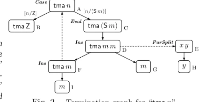
Example 3.2 (tma). An instantiation edge to˜t= (x y)is needed to obtain termination graphs for functions liketmawhich are applied to “toomany”arguments in recursive calls.¹³

tman

tma Z tma(Sm)

tmam m

m

[n/Z] [n/(Sm)]

x y y a

Case

b c

Eval

d

Ins

f

Ins

g i

e

ParSplit

h

Fig. 2. Termination graph for “tman”

tma :: Nats→a tma(Sm) =tmam m We get the termination graph in Figure 2. After applying Case andEval, we obtain “tmam m”

in node d which is not an instance of the start term “tman”

in node a. Of course, we could continue with Case and Eval

infinitely often, but to obtain a termination graph, at some point we need to apply theIns-rule. Here, the only possibility is to regardt= (tmam m) as an instance of the term˜t= (x y). Thus, we obtain an instantiation edge to the new nodee. As the instantiation is[x/(tmam), y/m], we get additional child nodesfandgmarked with “tmam” and m, respectively. Now we can “close” the graph, since “tmam”

is an instance of the start term “tman” in node a. So the instantiation edge to the special term(x y)is used to remove “superfluous” arguments (i.e., it effectively reduces the analysis of “tmam m” in node d to the analysis of “tmam” in node f). Of course, in any termination graph it suffices to have at most one node of the form “(x y)”. To expand the node “(x y)” further, one uses the ParSplit-rule to create its child node with the termy.

Theorem 3.3 shows that by the expansion rules of Definition 3.1 one can always obtain normal forms.¹⁴

Theorem 3.3 (Existence of Termination Graphs). The relation ⇛ is normalizing, i.e., for any termt there exists a termination graph.

4. FROM TERMINATION GRAPHS TO DP PROBLEMS

Now we present a method to prove H-termination of all terms in a termination graph. To this end, we want to use existing techniques for termination analysis of term rewriting. One of the most popular termination techniques for TRSs is the dependency pair (DP) method [Arts and Giesl 2000]. In particular, the DP method can be formulated as a general framework which permits the integration and combination ofany termination technique for TRSs [Giesl et al. 2005a; Giesl et al. 2006c; Hirokawa and Middeldorp 2005; 2007]. This DP framework operates on so-calledDP problems (P,R). Here,P andRare TRSs whereP may also have rulesℓ→rwherercontains extra variables not occurring inℓ. P’s rules are called

13Note thattmais not Hindley-Milner typeable (but has a principal type). Hence, Haskell can verify the given type oftma, but it cannot infer the type oftmaitself.

14All proofs can be found in the appendix.

(13)

dependency pairs. The goal of the DP framework is to show that there is no infinite chain, i.e., no infinite reduction s1σ1 →P t1σ1 →^∗_R s2σ2 →P t2σ2 →^∗_R . . . where si→ti∈ Pandσi are substitutions. In this case, the DP problem (P,R) is called finite. See e.g. [Giesl et al. 2005a; Giesl et al. 2006c; Hirokawa and Middeldorp 2005; 2007] for an overview of techniques to prove finiteness of DP problems.¹⁵

Instead of transforming termination graphs into TRSs, the information available in the termination graph can be better exploited if one transforms these graphs into DP problems.¹⁶ Then finiteness of the resulting DP problems impliesH-termination of all terms in the termination graph.

Note that termination graphs still contain higher-order terms (e.g., applications of variables to other terms like “x y” and partial applications like “takeu”). How- ever, most methods and tools for automated termination analysis only operate on first-order TRSs. Therefore, one option would be to translate higher-order terms intoapplicative first-order terms containing just variables, constants, and a binary symbol apfor function application, see [Kennaway et al. 1996; Giesl et al. 2005b;

Giesl et al. 2006a; Hirokawa et al. 2008]. Then terms like “x y”, “take u”, and

“take uxs” would be transformed into the first-order terms ap(x, y), ap(take, u), and ap(ap(take, u),xs), respectively. In Section 5, we will present a more sophis- ticated way to translate the higher-order terms from the termination graph into first-order terms. But at the moment, we disregard this problem and transform termination graphs into DP problems that may indeed contain higher-order terms.

Recall that if a node in the termination graph is marked with a non-H-terminating term, then one of its children is also marked with a non-H-terminating term. Hence, every non-H-terminating term corresponds to an infinite path in the termination graph. Since a termination graph only has finitely many nodes, infinite paths have to end in a cycle. Thus, it suffices to proveH-termination for all terms occurring instrongly connected components (SCCs)of the termination graph. Moreover, one can analyze H-termination separately for each SCC. Here, an SCC is a maximal subgraphG^′ of the termination graph such that for all nodesn1andn2inG^′ there is a non-empty path fromn1ton2traversing only nodes ofG^′. (In particular, there must also be a non-empty path from every node to itself in G^′.) The termination graph for “takeu(fromm)” in Figure 1 has just one SCC with the nodesa,c,e,f, h. The following definition is needed to generate dependency pairs from SCCs of the termination graph.

Definition 4.1 (DP Path). LetG^′ be an SCC of a termination graph containing a path from a node marked with s to a node marked with t. We say that this path is aDP pathif it does not traverse instantiation edges, if shas an incoming instantiation edge inG^′, and ifthas an outgoing instantiation edge inG^′.

So in Figure 1, the only DP path is a, c, e, f, h. Since every infinite path has to traverse instantiation edges infinitely often, it also has to traverse DP paths

15In the DP literature, one usually does not consider rules with extra variables on right-hand sides, but almost all existing termination techniques for DPs can also be used for such rules. (For example, finiteness of such DP problems can often be proved by eliminating the extra variables by suitableargument filterings[Arts and Giesl 2000; Giesl et al. 2005a].)

16We will discuss the disadvantages of a transformation into TRSs at the end of this section.

(14)

infinitely often. Therefore, we generate a dependency pair for each DP path. If there is no infinite chain with these dependency pairs, then no term corresponds to an infinite path, so all terms in the graph areH-terminating.

More precisely, whenever there is a DP path from a node marked with s to a node marked withtand the edges of the path are marked withσ1, . . . , σk, then we generate the dependency pairsσ1. . . σk →t. In Figure 1, the first edge of the DP path is labelled with the substitution [u/(Sn)] and all remaining edges are labelled with the identity. Thus, we generate the dependency pair

take(Sn) (fromm)→taken(from(Sm)). (1) The resulting DP problem is (P,R) where P = {(1)} and R = ∅.¹⁷ When using an appropriate translation into first-order terms as sketched above, automated termination tools (such as AProVE [Giesl et al. 2006b], TTT2 [Korp et al. 2009], and others) can easily show that this DP problem is finite. Hence, the start term

“takeu(fromm)” isH-terminating in the originalHaskell-program.

Similarly, finiteness of the DP problem ({tma(Sm)→ tmam},∅) for the start term “tman” from Figure 2 is also easy to prove automatically.

The construction of DP problems from the termination graph must be done in such a way that there is an infinite chain whenever the termination graph contains a non-H-terminating term. Indeed, in this case there also exists a DP path in the termination graph whose first node s is notH-terminating. We should construct the DP problems in such a way that salso starts an infinite chain. Clearly if sis notH-terminating, then there is a normal ground substitution σ where sσ is not H-terminating either. There must be a DP path fromsto a termtlabelled with the substitutions σ1, . . . , σk such thattσ is also notH-terminating and such thatσ is an instance ofσ1. . . σk (asσis anormalground substitution and the substitutions σ1, . . . , σk originate fromCase analyses that consider all possible constructors of a data type). So the first step of the desired corresponding infinite chain issσ→P tσ.

The nodethas an outgoing instantiation edge to a node ˜twhich starts another DP path. So to continue the construction of the infinite chain in the same way, we now need a non-H-terminating instantiation of ˜t with a normal ground substitution.

Obviously, ˜tmatchestby some matcherµ. But while ˜tµσis notH-terminating, the substitutionµσis not necessarily a normal ground substitution. The reason is that t and henceµmay contain defined symbols. The following example demonstrates this problem.

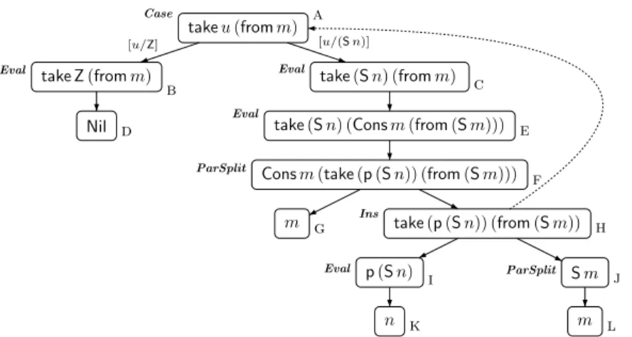
Example 4.2 (takewith p). A slightly more challenging example is obtained by replacing the last take-rule in Example 2.1 by the following two rules, where p computes thepredecessor function.

take(Sn) (Consxxs) =Consx(take(p(Sn))xs) p(Sx) =x

We consider the start term “takeu(fromm)” again. The resulting termination graph is shown in Figure 3. The only DP path isa,c,e,f, h, which would result in the dependency pairtake(Sn) (fromm)→twith t=take(p(Sn)) (from(Sm)).

Nowt has an instantiation edge to node awith ˜t=takeu(fromm). The matcher isµ= [u/(p(Sn)), m/(Sm)]. Soµ(u)is not normal.

17Definition 4.9 will explain how to generateRin general.

(15)

Nil

take(Sn) (fromm) take(Sn) (Consm(from(Sm))) Consm(take(p(Sn)) (from(Sm)))

m take(p(Sn)) (from(Sm))

p(Sn) Sm

n m

[u/Z] [u/(Sn)]

a

Case

b

Eval

c

Eval

d

Eval

e

ParSplit f

g ^Ins h

Eval i

ParSplit j

k l

Fig. 3. Termination graph for new “takeu(fromm)”

In Example 4.2, the problem of defined symbols in right-hand sides of dependency pairs can be avoided by already evaluating the right-hand sides of dependency pairs as much as possible. To this end, we define an appropriate function ev. Before presenting the formal definition ofevin Definition 4.4, we will motivate it step by step. More precisely, we will discuss howev(t) should be defined for different kinds of nodest.

So instead of a dependency pair sσ1. . . σk → t we now generate the dependency pair sσ1. . . σk →ev(t). For a node marked with t, essentially ev(t) is the term reachable from tby traversing only Eval-nodes. So in our example we have ev(p(Sn)) =n, since nodeiis anEval-node with an edge to nodek. Moreover, we will defineevin such a way thatev(t) can also evaluate subterms oftiftis anIns- node or aParSplit-node with a constructor as head. We obtainev(Sm) =Smfor node j and ev(take(p(Sn)) (from(Sm))) =taken(from(Sm)) for node h. Thus, the resulting DP problem is again (P,R) withP={(1)}andR=∅.

nontermb x nonterm Truex

True

nonterm Falsex nonterm(xTrue)x

xTrue x

True

[b/True] [b/False]

a

Case

b

Eval ^Eval c

d ^Ins e

ParSplit f

g h

Fig. 4. Termination graph for “nontermb x”

To show how ev(t) should be defined for ParSplit-nodes where head(t) is a variable, we consider the function nonterm from Example 2.5 again. The termination graph for the start term “nontermb x” is given in Figure 4. We obtain a DP path from

node awith the start term to node e with “nonterm(xTrue)x” labelled with the substitution [b/False]. So the resulting DP problem only contains the dependency pair “nonterm Falsex→ev(nonterm(xTrue)x)”. If we definedev(xTrue) =xTrue, then ev would not modify the term “nonterm(xTrue)x”. But then the resulting DP problem would be finite and one could falsely proveH-termination. (The reason is that the DP problem contains no rule to transform any instance of “xTrue”

to False.) But as discussed in Section 3, x can be instantiated by arbitrary H-

(16)

terminating functions and then, “xTrue” can evaluate to any term of type Bool.

Therefore, we should defineevin such a way that it replaces subterms like “xTrue”

by fresh variables.

LetU_G be the set of all ParSplit-nodes¹⁸ with variable heads in a termination graphG. In other words, this set contains nodes whose evaluations can lead to any term of a given type.

U_G ={t|tis aParSplit-node in Gwitht= (x t1 . . . tn)}

Recall that iftis anIns-node or aParSplit-node with a constructor head, then evproceeds by evaluating subterms oft. More precisely, lett= ˜t[x1/s1, ..., xm/sm], where either ˜t = (c x1. . . xm) for a constructor c (then t is a ParSplit-node) or t is an Ins-node and there is an instantiation edge to ˜t. In both cases, t also has the children s1, . . . , sm. As mentioned before, we essentially define ev(t) =

˜t[x1/ev(s1), . . . , xm/ev(sm)]. However, whenever there is a path fromsito a term from U_G (i.e., to a term (x . . .) that ev approximates by a fresh variable), then instead ofev(si) one should use a fresh variable in the definition ofev(t). A fresh variable is needed because then an instantiation ofsi could in principle evaluate to any value.

Example 4.3 (evfor Ins-nodes). Consider the following program:

fx z f Zz

f(idzZ)z z

idzZ x y

idz Z y

z

f(Sn)z

[x/Z]

[x/(Sn)]

a

Case b

Eval c

d

Ins e

f

Ins ^ParSplit g

Eval h

i j

k

Fig. 5. Termination graph for “fx z”

f Zz=f(idzZ)z idx=x The termination graph for the start term

“fx z” is depicted in Figure 5. From the DP path a, c, d, we obtain the dependency pair

“f Z z → ev(f (id z Z) z)”. Note that node d is an Ins-node where (f (id z Z) z) = (fx z) [x/(idzZ), z/z], i.e., here we have ˜t = (fx z).

If one definedevonIns-nodes by simply applying it to the child-subterms, then we would get ev(f (id z Z) z) = f ev(id z Z) ev(z).

Clearly, ev(z) = z. Moreover, (id z Z) (i.e.,

node f) is again an Ins-node where (id z Z) = (x y) [x/(id z), y/Z]. Thus, ev(id z Z) = ev(id z) ev(Z) = z Z. Hence, the resulting dependency pair

“f Z z → ev(f (id z Z) z)” would be “f Z z → f (z Z) z”. The resulting DP problem would contain no rules R. As this DP problem is finite, then we could falsely proveH-termination off.

However, there is a path from node f with the child-subterm (id z Z) to node g with the term (x y) which is in U_G. As discussed above, when computing ev(f (id z Z) z), ev should not be applied to child-subterms like f, but instead, one should replace such child-subterms by fresh variables. So we obtain ev(f (id z Z) z) = f u z for a fresh variable u. The resulting dependency pair f Zz→fu zindeed gives rise to an infinite chain.

Let the setPU_G contain all nodes from which there is a path to a node inU_G.

18To simplify the presentation, we identify nodes with the terms they are labelled with.

(17)

So in particular, we also haveU_G ⊆PU_G. For instance, in Example 4.3 we have U_G={g} andPU_G={a,c,d,f,g}. Now we can define evformally.

Definition 4.4 (ev). LetGbe a termination graph with a nodet. Then

ev(t) =











x, for a fresh variablex, ift∈UG

t, iftis a leaf, aCase-node, or aVarExp-node ev(˜t), iftis anEval-node with child˜t

˜t[x1/t1, . . . , xm/tm],

ift= ˜t[x1/s1, . . . , xm/sm]and

•tis anIns-node with the childrens1, . . . , sm,˜tor

tis a ParSplit-node,˜t= (c x1. . . xm)for a constructorc

•ti =

yi, for a fresh variableyi, ifsi∈PU_G ev(si), otherwise

Our goal was to construct the DP problems in such a way that there is an infinite chain whenevers is the first node in a DP path andsσis notH-terminating for a normal ground substitution σ. As discussed before, then there is a DP path from s to t such that the chain starts with sσ→P ev(t)σ and such that tσ and hence ev(t)σ is also not H-terminating. The node t has an instantiation edge to some node ˜t. Thus, t = ˜t[x1/s1, . . . , xm/sm] and ev(t) = ˜t[x1/ev(s1), . . . , xm/ev(sm)], if we assume for simplicity that the siare not fromPU_G.

In order to continue the construction of the infinite chain, we need a non-H- terminating instantiation of ˜t with a normal ground substitution. Clearly, if ˜t is instantiated by the substitution [x1/ev(s1)σ, . . . , xm/ev(sm)σ], then it is again notH-terminating. However, the substitution [x1/ev(s1)σ, . . . , xm/ev(sm)σ] is not necessarily normal. The problem is thatev stops performing evaluations as soon as one reaches a Case-node (i.e., ev is not propagated over edges originating in Case-nodes). A similar problem is due to the fact thatevis also not propagated over instantiation edges.

Therefore, we now generate DP problems which do not just contain dependency pairsP, but they also contain all rulesRwhich might be needed to evaluateev(si)σ further. Then we obtain sσ→P ev(t)σ→^∗_R ˜tσ^′ for a normal ground substitution σ^′ where ˜tσ^′is notH-terminating. Since ˜tis again the first node in a DP path, now this construction of the chain can be continued in the same way infinitely often.

Hence, we obtain an infinite chain.

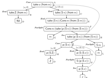
Example 4.5 (takewith recursivep). To illustrate this, we replace the equation forpin Example 4.2 by the following two defining equations:

p(S Z) =Z p(Sx) =S(px)

For the start term “takeu(fromm)”, we obtain the termination graph depicted in Figure 6. Soiis now a Case-node. Thus, instead of (1) we have the dependency pair

take(Sn) (fromm) → take(p(Sn)) (from(Sm)), (2) since now ev(p(Sn)) = p(Sn). Hence, the resulting DP problem must contain all rules Rthat might be used to evaluate p(Sn)when instantiated by a normal ground substitutionσ.

(18)

Nil

take(Sn) (fromm) take(Sn) (Consm(from(Sm))) Consm(take(p(Sn)) (from(Sm)))

m take(p(Sn)) (from(Sm)) Sm

m

[u/Z] [u/(Sn)]

Case a

b

Eval

c

Eval

d

Eval

e

ParSplit f

g h

Ins

ParSplit j l p(Sn)

p(S Z) p(S(Sx))

Z S(p(Sx))

p(Sx) x

[n/Z] [n/(Sx)]

Case i

m

Eval

n

Eval

o p

ParSplit

q

Ins

r

Fig. 6. Termination graph for “takeu(fromm)” with modifiedp-equations

So for any termt, we want to detect the rules that might be needed to evaluate ev(t)σ further for normal ground substitutions σ. To this end, we first compute the setcon(t) of those terms that are reachable fromt, but where the computation ofev stopped. In other words,con(t) contains all terms which might give rise to further continuing evaluations that are not captured byev. To compute con(t), we traverse all paths starting int. If we reach aCase-nodes, we stop traversing this path and insert sinto con(t). Moreover, if we traverse an instantiation edge to some node ˜t, we also stop and insert ˜tinto con(t). So in the example of Figure 6, we obtain con(p(Sn)) = {p(Sn)}, since i is now a Case-node. If we had started with the term t =take(Sn) (fromm) in nodec, then we would reach the Case-node i and the node a which is reachable via an instantiation edge. So con(t) = {p(Sn),takeu(fromm)}. Moreover, con also stops at leaves and at VarExp-nodest, since they are in normal form w.r.t. →H. Thus, herecon(t) =∅. Finally, note thatconis initially applied toIns-nodes (i.e., to terms on right-hand sides of dependency pairs). Hence, if a (sub)term t is in PUG, then ev already approximates the result oft’s evaluation by a fresh variable. Thus, one also defines con(t) =∅for allt∈PUG.

Definition 4.6 (con). LetGbe a termination graph with a nodet. Then

con(t) =











∅, ift is a leaf or aVarExp-node ort∈PU_G {t}, ift is aCase-node

{t} ∪˜ con(s1)∪. . .∪con(sm), ift is anIns-node with

the childrens1, . . . , sm,˜t and an instantiation edge fromt to˜t S

t^′child oft con(t^′), otherwise

Now we can define how to extract a DP problem dp_G′ from every SCC G^′ of