Bytecode Programs by Term Rewriting ∗
Marc Brockschmidt, Carsten Otto, Jürgen Giesl
LuFG Informatik 2, RWTH Aachen University, Germany
Abstract
In [5, 15] we presented an approach to prove termination of non-recursiveJava Bytecode(JBC) pro- grams automatically. Here,JBCprograms are first transformed to finitetermination graphswhich represent all possible runs of the program. Afterwards, the termination graphs are translated to term rewrite systems (TRSs) such that termination of the resulting TRSs implies termination of the originalJBC programs. So in this way, existing techniques and tools from term rewriting can be used to prove termination of JBCautomatically. In this paper, we improve this approach substantially in two ways:
(1) We extend it in order to also analyze recursive JBC programs. To this end, one has to represent call stacks of arbitrary size.
(2) To handleJBC programs with several methods, wemodularizeour approach in order to re- use termination graphs and TRSs for the separate methods and to prove termination of the resulting TRS in a modular way.
We implemented our approach in the tool AProVE. Our experiments show that the new contri- butions increase the power of termination analysis forJBCsignificantly.
1998 ACM Subject Classification D.1.5 - Object-oriented Programming, D.2.4 - Software/Pro- gram Verification, D.3.3 - Language Constructs and Features, F.3 - Logics and Meanings of Programs, F.4.2 - Grammars and Other Rewriting Systems, I.2.2 - Automatic Programming Keywords and phrases termination,Java Bytecode, term rewriting, recursion
Digital Object Identifier 10.4230/LIPIcs.xxx.yyy.p Category Regular Research Paper
1 Introduction
While termination of TRSs and logic programs was studied for decades, recently there have also been many results on termination ofimperative programs (e.g., [3, 6, 7, 8]). However, these methods do not re-use the many existing termination techniques for TRSs and declar- ative languages. Therefore, in [5, 15] we presented the first rewriting-based approach for proving termination of a real imperative object-oriented language, viz.Java Bytecode[14].
We only know of two other automated methods to analyzeJBCtermination, implemented in the toolsCOSTA[2] andJulia[16]. They transform JBCinto a constraint logic program by abstracting objects of dynamic data types to integers denoting their path-length (e.g., list objects are abstracted to their length). While this fixed mapping from objects to integers leads to high efficiency, it also restricts the power of these methods.
In contrast, in [5, 15] we represent data objects not by integers, but bytermswhich express as much information as possible about the objects. For example, list objects are represented by terms of the formList(t1,List(t2, . . .List(tn,null). . .)). In this way, we benefit from the fact
∗ Supported by the DFG grant GI 274/5-3 and the G.I.F. grant 966-116.6.
© M. Brockschmidt, C. Otto, J. Giesl;
that rewrite techniques can automatically generate well-founded orders comparing arbitrary forms of terms. Moreover, by using TRSs with built-in integers [9], our approach is not only powerful for algorithms on user-defined data structures, but also for algorithms on pre-defined data types like integers. To obtain TRSs that are suitable for termination analysis, our approach first transforms a JBC program into a termination graph which represents all possible runs of the program. These graphs handle all aspects of JBC that cannot easily be expressed in term rewriting (e.g., side effects, cyclic data objects, object-orientation, etc.).
Afterwards, a TRS is generated from the termination graph. As proved in [5, 15], termination of this TRS implies termination of the originalJBCprogram.
We implemented this approach in our toolAProVE[10] and in the International Termin- ation Competitions,1 AProVEachieved competitive results compared to JuliaandCOSTA.
However, a significant drawback was that (in contrast to techniques that abstract objects to integers [2, 8, 16]), our approach in [5, 15] could not deal withrecursion. The problem is that for recursive methods, the size of the call stack usually depends on the input arguments.
Hence, to represent all possible runs, this would lead to termination graphs with infinitely many states (since [5, 15] used no abstraction on call stacks). An abstraction of call stacks is non-trivial due to possible aliasing between references in different stack frames.
In the current paper, we solve these problems. Instead of directly generating a termination graph for the whole program as in [5, 15], in Sect. 2 we construct a separate termination graph for each method. These graphs can be combined afterwards. Similarly, one can also combine the TRSs resulting from these “method graphs” (Sect. 3). As demonstrated by our implementation inAProVE(Sect. 4), our new approach has two main advantages over [5, 15]:
(1) We can now analyzerecursivemethods, since our new approach can deal with call stacks that may grow unboundedly due to method calls.
(2) We obtain amodular approach, because one can re-use a method graph (and the rewrite rules generated from it) whenever the method is called. So in contrast to [5, 15], now we generate TRSs that are amenable to modular termination proofs.
See [4] for all proofs, and see [1] for experimental details and our previous papers [5, 15].
2 From Recursive JBC to Modular Termination Graphs
To analyze termination of a set of desired initial (concrete) program states, we represent this set by a suitableabstract statewhich is the initial node of the termination graph. Then this state isevaluated symbolically, which leads to its child nodes in the termination graph.
Our approach is restricted to verified2 sequentialJBCprograms. To simplify the present- ation in this paper, we exclude arrays, static class fields, interfaces, and exceptions. We also do not describe the annotations introduced in [5, 15] to handle complex sharing effects. With such annotations one can for example also model “unknown” objects with arbitrary sharing behavior as well as cyclic objects. Extending our approach to such constructs is easily possi- ble and has been done for our implementation in the termination proverAProVE. However, cur- rently our implementation has only minimal support for features like floating point arithmetic, strings, static initialization of classes, instances of java.lang.Class, reflection, etc.
Sect. 2.1 presents our notion ofstates. Sect. 2.2 introduces termination graphsfor one method and Sect. 2.3 shows how to re-use these graphs for programs with many methods.
1 Seehttp://www.termination-portal.org/wiki/Termination_Competition.
2 The bytecode verifier of theJVM[14] ensures certain properties of the code that are useful for our analysis, e.g., that there is no overflow or underflow of the operand stack.
2.1 States
f i n a l c l a s s L i s t { L i s t n ;
p u b l i c v o i d a p p E (i n t i ) { if ( n == n u l l) {
if ( i <= 0) r e t u r n; n = n e w L i s t ();
i - -;
}
n . a p p E ( i );
}}
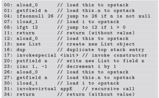
00: a l o a d _ 0 // l o a d t h i s to o p s t a c k 01: g e t f i e l d n // l o a d t h i s . n to o p s t a c k 04: i f n o n n u l l 26 // j u m p to 26 if n is not n u l l 07: i l o a d _ 1 // l o a d i to o p s t a c k
08: i f g t 12 // j u m p to 12 if i > 0 11: r e t u r n // r e t u r n ( w i t h o u t v a l u e ) 12: a l o a d _ 0 // l o a d t h i s to o p s t a c k 13: new L is t // c r e a t e new L i s t o b j e c t 16: dup // d u p l i c a t e top s t a c k e n t r y 17: i n v o k e s p e c i a l < init > // i n v o k e c o n s t r u c t o r 20: p u t f i e l d n // w r i t e new L i s t to f i e l d n 23: i i n c 1 , -1 // d e c r e m e n t i by 1
26: a l o a d _ 0 // l o a d th i s to o p s t a c k 27: g e t f i e l d n // l o a d t h i s . n to o p s t a c k 30: i l o a d _ 1 // l o a d i to o p s t a c k 31: i n v o k e v i r t u a l a p p E // r e c u r s i v e c a l l 34: r e t u r n // r e t u r n ( w i t h o u t v a l u e )
Consider the recursive method appE (presented in both Java and JBC). We use a class List where the field n points to the next list
element. For brevity, we omitted a field for the value of a list element. The methodappE recursively traverses the list to its end, where it attachesifresh elements (ifi > 0).
o1, i3|0|t:o1,i:i3|ε o1:List(n=o2) i3:Z o2:List(?)
Figure 1 State Fig. 1 displays an abstract state of appE. A state consists of a
sequence of stack frames and the heap, i.e., States =SFrames∗
×Heap. The state in Fig. 1 has just a single stack frame “o1, i3|0| t:o1,i:i3|ε” which consists of four components. Its first component
o1, i3are theinput arguments, i.e., those objects that are “visible” from outside the analyzed method. This component is new compared to [5, 15] and it is needed to denote later on which of these objects have been modified by side effects during the execution of the method. In our example,appEhas two input arguments, viz. the implicit formal parameterthis(whose value iso1) and the formal parameteriwith valuei3. In contrast toJBC, we also represent integers by references and adapt the semantics of all instructions to handle this correctly. So o1, i3∈Refs, whereRefsis an infinite set of names for addresses on the heap.
The second component0of the stack frame is theprogram position (fromProgPos), i.e., the index of the next instruction. So0means that evaluation continues withaload_0.
The third component is the list of values of local variables, i.e.,LocVar=Refs∗. To ease readability, we do not only display the values, but also the variable names. For example, the name of the first local variablethisis shortened totand its value iso1.
The fourth component is theoperand stack to store temporary results, i.e.,OpStack= Refs∗. Here,εis the empty stack and “o8, o1” denotes a stack witho8on top.
So the set of allstack framesisSFrames=InpArgs×ProgPos×LocVar×OpStack. As mentioned, the call stack of a state can consist of several stack frames. If a method calls another method, then a new frame is put on top of the call stack.
In addition to the call stack, a state contains information on theheap. The heap is a partial function mapping references to their value, i.e.,Heap=Refs→Integers∪Instances∪ Unknown∪{null}. We depict a heap by pairs of a reference and a value, separated by “:”.
Integers are represented by intervals, i.e., Integers = {{x ∈ Z | a ≤ x ≤ b} | a ∈ Z∪ {−∞}, b∈Z∪ {∞}, a≤b}. We abbreviate (−∞,∞) byZ, [1,∞) by [>0], etc. So “i3: Z” means that any integer can be at the addressi3. Since current TRS tools cannot handle 32-bitint-numbers, we treat all numeric types likeintas the infinite set of all integers.
To representInstances(i.e., objects) of some class, we store their type and the values of their fields, i.e.,Instances=Classnames×(FieldIDs→Refs). Classnamescontains the names of all classes. FieldIDsis the set of all field names. To prevent ambiguities, in general theFieldIDsalso include the respective class name. For all (cl, f)∈Instances, the functionf is defined for all fields ofcl and of its superclasses. Thus, “o1:List(n=o2)”
means that at the address o1, there is aList object whose fieldnhas the valueo2.
Unknown=Classnames×{?}representsnulland all tree-shaped objects for which we only have type information. In particular, Unknownobjects are acyclic and do not share parts of the heap with any objects at the other references in the state. For example,
“o2:List(?)” means thato2 isnull or an instance ofList (or a subtype ofList).
Everyinput argument has a boolean flag, wherefalse indicates that it may have been modified (as a side effect) by the current method. Moreover, we store which formal parameter of the method corresponds to this input argument. So in Fig. 1, the full input arguments are (o1,lv0,0,true) and (i3,lv0,1,true). Here,lvi,j is theposition of thej-th local variable in thei-th stack frame. When the top stack frame (i.e., frame 0) is at program position 0of a method, then its 0-th and 1-st local variables (at positionslv0,0andlv0,1) correspond to the first and second formal parameter of the method. Formally,InpArgs= 2Refs×SPos×B. Astate position π∈SPos(s) is a sequence starting withlvi,j,osi,j (for operand stack entries), orini,τ (for input arguments (r, τ, b) in thei-th stack frame), followed by a sequence ofFieldIDs. This sequence indicates how to access a particular object.
IDefinition 1(State Positions). Lets= (hfr0, . . . ,frni, h)∈Stateswherefri= (ini, ppi, lvi, osi). ThenSPos(s) is the smallest set containing all the following sequences π:
π=lvi,j where 0≤i≤n,lvi=hl0, . . . , lmi, 0≤j≤m. Thens|π islj. π=osi,j where 0≤i≤n,osi =ho0, . . . , oki, 0≤j≤k. Thens|π isoj. π=ini,τ where 0≤i≤nand (r, τ, b)∈ini. Thens|π isr.
π = π0v for some v ∈ FieldIDs and some π0 ∈ SPos(s) where h(s|π0) = (cl, f) ∈ Instancesand wheref(v) is defined. Thens|π isf(v).
Thereferences in the statesare defined asRef(s) ={s|π|π∈SPos(s)}.
So for the statesin Fig. 1, we haves|lv0,0 =s|in0,lv0,0 =o1,s|lv0,0n=s|in0,lv0,0n=o2, etc.
2.2 Termination Graphs for a Single Method
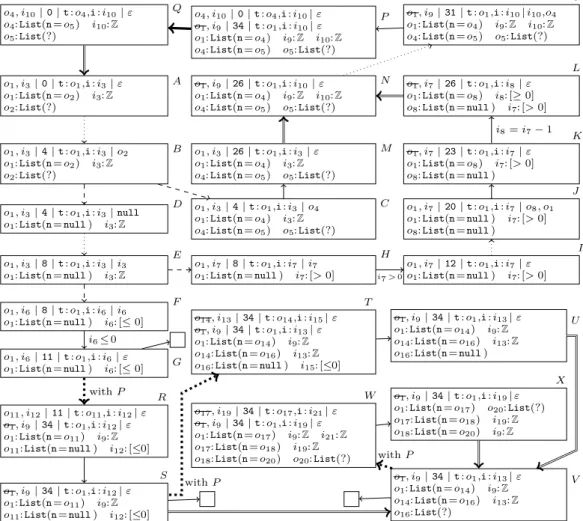
In Fig. 2, we construct the termination graph ofappE. The state in Fig. 1 is its initial state A, i.e., we analyze termination ofappEfor acyclic lists of arbitrary length and any integer.
InA,aload_0loads the value of the 0-th local variablethis on the operand stack. So A is connected by anevaluation edge to a state with program position 1 (omitted from Fig. 2 due to space reasons, i.e., dotted arrows abbreviateseveral steps). Then “getfield n” replaceso1on the operand stack by the value o2 of its fieldn, resulting in stateB. The valueList(?) ofo2does not provide enough information to evaluateifnonnull. Thus, we perform aninstance refinement [5, Def. 5] resulting inC andD, i.e., a case analysis whether o2’s value isnull. Refinement edges are denoted by dashed lines. InC, we assume thato2’s value is notnull. Thus, we replaceo2by a fresh3 referenceo4, which points toList(n=o5).
Hence, we can now evaluateifnonnulland jump to instruction26in stateM.
InD, we assume that o2’s value isnull, i.e., “o1:List(n=o2)” and “o2 :null”. To ease the presentation, in such states we simply replace all occurrences ofo2withnull. After evaluating the instruction “ifnonnull 26”, in the next state (which we omitted from Fig. 2 for space reasons), the instruction “iload_1” loads the value ofion the operand stack. This results in stateE. Now again we do not have enough information to evaluateifgt. Thus, we perform aninteger refinement [5, Def. 1], leading to statesF (ifi <= 0) andH.
3 We rename references that are refined to ease the formal definition of the refinements, cf. [5].
o1, i3|0|t:o1,i:i3|ε o1:List(n=o2) i3:Z o2:List(?)
A
o1, i3|4|t:o1,i:i3|o2 o1:List(n=o2) i3:Z o2:List(?)
B
o1, i3|4|t:o1,i:i3|o4
o1:List(n=o4) i3:Z o4:List(n=o5) o5:List(?)
C o1, i3|4|t:o1,i:i3|null
o1:List(n=null) i3:Z
D
o1, i3|8|t:o1,i:i3|i3
o1:List(n=null) i3:Z
E
o1, i6|8|t:o1,i:i6|i6
o1:List(n=null) i6: [≤0]
F
o1, i6|11|t:o1,i:i6|ε
o1:List(n=null) i6: [≤0] G
o1, i7|8|t:o1,i:i7|i7
o1:List(n=null) i7: [>0]
H
o1, i7|12|t:o1,i:i7|ε o1:List(n=null) i7: [>0]
I o1, i7|20|t:o1,i:i7|o8, o1
o1:List(n=null) i7: [>0]
o8:List(n=null)
J o1, i7|23|t:o1,i:i7|ε o1:List(n=o8) i7: [>0]
o8:List(n=null)
K o1, i7|26|t:o1,i:i8|ε o1:List(n=o8) i8: [≥0]
o8:List(n=null) i7: [>0]
L
o1, i3|26|t:o1,i:i3|ε o1:List(n=o4) i3:Z o4:List(n=o5) o5:List(?)
M o1, i9|26|t:o1,i:i10|ε
o1:List(n=o4) i9:Z i10:Z o4:List(n=o5) o5:List(?)
N
o1, i9|31|t:o1,i:i10|i10,o4 o1:List(n=o4) i9:Z i10:Z o4:List(n=o5) o5:List(?)
O o4, i10|0|t:o4,i:i10|ε
o1, i9|34|t:o1,i:i10|ε o1:List(n=o4) i9:Z i10:Z o4:List(n=o5) o5:List(?) o4, i10|0|t:o4,i:i10|ε P
o4:List(n=o5) i10:Z o5:List(?)
Q
o11, i12|11|t:o11,i:i12|ε o1, i9|34|t:o1,i:i12|ε o1:List(n=o11) i9:Z o11:List(n=null) i12: [≤0]
R
o1, i9|34|t:o1,i:i12|ε o1:List(n=o11) i9:Z o11:List(n=null) i12: [≤0]
S
o14, i13|34|t:o14,i:i15|ε o1, i9|34|t:o1,i:i13|ε o1:List(n=o14) i9:Z o14:List(n=o16) i13:Z o16:List(n=null) i15: [≤0]
T
o1, i9|34|t:o1,i:i13|ε o1:List(n=o14) i9:Z o14:List(n=o16) i13:Z o16:List(n=null)
U
o1, i9|34|t:o1,i:i13|ε o1:List(n=o14) i9:Z o14:List(n=o16) i13:Z o16:List(?)
V o17, i19|34|t:o17,i:i21|ε
o1, i9|34|t:o1,i:i19|ε o1:List(n=o17) i9:Z i21:Z o17:List(n=o18) i19:Z o18:List(n=o20) o20:List(?)
W o1, i9|34|t:o1,i:i19|ε o1:List(n=o17) o20:List(?) o17:List(n=o18) i19:Z o18:List(n=o20) i9:Z
X i6≤0
i7>0
i8=i7−1
withP
withP
withP
Figure 2Termination Graph ofappE
In F, we evaluateifgt, leading toG. We label the edge fromF toGwith the condition i6 ≤0 of this case. This label will be used when generating a TRS from the termination graph. States likeGthat have only a single stack frame which is at areturnposition are called return states. Thus, we reach aprogram end, denoted by . From H, we jump to instruction12inI and label the edge withi7>0. InI, o1is pushed on the operand stack.
Afterwards, we create another list elemento8, where we skipped the constructor call in Fig. 2.
InK,o8has been written to the fieldnofo1. This is aside effecton an object that is visible from outside the method (sinceo1 is an input argument). Hence, inK we set the boolean flag foro1 tofalse (depicted by crossing out the input argumento1).
In L, the value of the 1-st local variable iis decremented by 1. In contrast to JBC, we represent primitive data types by references. Hence, we introduce a fresh referencei8, pointing to the adapted value. Sincei7’s value did not change,i7 is not crossed out.
StateLis similar to the stateM we obtained from the other branch of our first refinement.
To simplify the graph, we create ageneralized stateN, which represents a superset of all concrete states represented byL orM. N is almost likeM (up to renaming of references) and only differs in the information about input arguments, which is taken fromL. We draw instance edges (double arrows) fromLandM toN and only considerN in the remainder.
InO, we have loadedthis.nandion the operand stack and invokeappEon these values.
So inP, a second stack frame is pushed on top of the previous one. States likeP that contain at least two frames where the top frame is at the start of a method arecall states.
We now introduce a new approach to represent call stacks of arbitrary size bysplitting up call stacks. Otherwise, for recursive methods the call stack could grow unboundedly and we would obtain an infinite termination graph. SoP has a call edge(thick arrow) toQwhich only containsP’s top stack frame. SinceQis identical toA(modulo renaming), we do not have to analyzeappEagain, but simply draw an instance edge fromQtoA.
Up to nowAonly represented concrete states whereappEwas called “directly”. However, nowAcan also be reached from a “method call” inP. Hence, nowAand the other abstract statessofappE’s termination graph also represent states whereappEwas called “recursively”, i.e., where below the stack frames ofs, one has the stack frames ofP (onlyP’s top frame is replaced by the frames ofs).4 For eachreturn statewe now consider two cases: Either there are no further frames below the top frame (then one reaches a leaf of the termination graph) or else, there are further frames below the top (which result from the method call inP). Hence, for every return state likeG, we now create an additional successor stateR (thecontext concretization ofGwithP), connected by acontext concretization edge(a thick dotted arrow). R has the same stack frame asG(up to renaming), but below we add the call stack ofP (withoutP’s top frame that corresponded to the method call).
InR,appE’s recursive call has just reached thereturnstatement at index11. Here, we identifiedo1 andi6 from stateGwith o4 andi10from P and renamed them to o11 andi12. We now consider which information we have aboutR’s heap. According to stateG, the input arguments ofappE’s recursive call were not modified during the execution of this recursive call. Thus, for the input argumentso11 andi12 inR, we can useboth the information on o1 andi6 inGand ono4 andi10inP. According toG, o1 is a list of length 1 andi6≤0.
According to P,o4has at least length 1 andi10 is arbitrary. Hence, inRwe can take the intersection of this information and deduce thato11has length 1 and i12≤0. (So in this example, the intersection ofG’s andP’s information coincides with the information inG.)
When constructing termination graphs, context concretization is only needed for return states. But to formulate Thm. 3 on the soundness of termination graphs later on, in Def. 2 we introduce context concretization for arbitrary states s = (hfr0, . . . ,frni, h). So s re- sults from evaluating the method in the bottom framefrn (i.e.,frn−1 was created by a call infrn,frn−2 was created by a call infrn−1, etc.). Context concretization ofswith a call states= (hfr0, . . . ,frmi, h) means that we consider the case wherefrn results from a call in fr1. Thus, the top framefr0 ofsis at the start of some method and the bottom framefrn of smust be at an instruction of thesamemethod. Moreover, for all input arguments (r, τ, b) in fr0there must be acorresponding input argument (r, τ, b) infrn.5 To ease the formalization, let Ref(s) and Ref(s) be disjoint. For instance, if s is G and s is P, we can mark the references byG andP to achieve disjointness (e.g.,oG1 ∈Ref(G) andoP1 ∈Ref(P)).
Then we add the framesfr1, . . . ,frmof the call statesbelow the call stack ofsto obtain a new state ˜swith the call stack hfr0σ, . . . ,frnσ,fr1σ, . . . ,frmσi. Theidentification substi- tutionσidentifies every input argumentrof fr0 with the corresponding input argumentr offrn. If the boolean flag for the input argumentrinsis false, then this object may have changed during the evaluation of the method and in ˜s, we should only use the information
4 For example,Anow represents all states with call stackshfrA,frP1,frP1, . . . ,frP1iwherefrAisA’s stack frame andfrP1,frP1, . . . ,frP1 are copies ofP’s bottom frame (in which references may have been renamed).
SoArepresents states whereappEwas called within an arbitrary high context of recursive calls.
5 This obviously holds for all input arguments corresponding to formal parameters of the method, but Sect. 2.3 will illustrate that sometimesfr0may have additional input arguments.
froms. But if the flag istrue, then the object did not change. Then, both the information in sand insabout this object is correct and for ˜s, we take the intersection of this information.
In our example,σ(oG1) =σ(oP4) =oR11andσ(iG6) =σ(iP10) =iR12. Since the flags of the input argumentsoG1 andiG6 aretrue, foroR11 andiR12, we intersect the information fromGandP. If we identifyrandr, and both point toInstances, then we may also have to identify the references in their fields. To this end, we define an equivalence relation≡ ⊆Refs×Refs where “r≡r” means thatrandrare identified. Letr≡rand letrbe no input argument in swith the flagfalse. Ifrpoints to (cl, f) insandrpoints to (cl, f) ins, then all references in the fields vofcl and its superclasses also have to be identified, i.e., f(v)≡f(v).
To illustrate this in our example, note that we abbreviated the information onG’s heap in Fig. 2. In reality we have “oG1 :List(n=oG2)”, “oG2 :null”, and “iG6 : [≤0]”. Hence, we do not only obtainiG6 ≡iP10 andoG1 ≡oP4, but sinceoG1’s boolean flag is notfalse, we also have to identify the references at the fieldnof the object, i.e.,oG2 ≡oP5.
Letρbe an injective function that maps each≡-equivalence class to a fresh reference. We define theidentification substitutionσasσ(r) =ρ([r]≡) for allr∈Ref(s)∪Ref(s). So we map equivalent references to the same new reference and we map non-equivalent references to different references. To construct ˜s, ifr∈Ref(s) points to an object which was not modified by side effects during the execution of the called method (i.e., where the flag is notfalse), we intersect all information insandson the references in [r]≡. For all other references in Ref(s) resp.Ref(s), we only take the information fromsresp.sand applyσ.
In our example, we have the equivalence classes {oG1, oP4}, {oG2, oP5}, {iG6, iP10}, {oP1}, and{iP9}. For these classes we choose the new references oR11, oR2, iR12, oR1, iR9, and obtain σ={oG1/oR11, oP4/oR11, oG2/oR2, oP5/oR2, iG6/iR12, iP10/iR12, oP1/oR1, iP9/iR9}. The information foroR11, oR2, and iR12 is obtained by intersecting the respective information from G and P. The information foroR1 andiR9 is taken over fromP (by applyingσ).
Def. 2 also introduces the concept of intersection formally. Ifr∈Refs(s), r∈Refs(s), and h resp. h are the heaps of s resp. s, then intuitively, h(r)∩h(r) consists of those values that are represented by bothh(r) andh(r). For example, ifh(r) = [≥0] = (−1,∞) andh(r) = [≤0] = (−∞,1), then the intersection is (−1,1) = [0,0]. Similarly, if h(r) or h(r) isnull, then their intersection is againnull. Ifh(r), h(r) areUnknowninstances of classes cl1,cl2, then their intersection is an Unknowninstance of the more special class min(cl1,cl2). Here, min(cl1,cl2) =cl1ifcl1 is a (not necessarily proper) subtype ofcl2 and min(cl1,cl2) =cl2 ifcl2 is a subtype ofcl1. Otherwise,cl1 andcl2 are calledorthogonal. If h(r)∈Unknownandh(r)∈Instances, then their intersection is fromInstances using the more special type. Finally, if bothh(r), h(r)∈Instanceswith the same type, then their intersection is again fromInstances. For the references in its fields, we use the identification substitutionσthat renames equivalent references to the same new reference.
Note that one may also have to identify different references in the same state. For example, scould have the input arguments (r, τ1, b) and (r, τ2, b) with the corresponding input arguments (r1, τ1, b1) and (r2, τ2, b2) in s. Thenr ≡r1 ≡r2. Note that if r1 6=r2
are references from thesamestate where h(r1)∈Instances, then they point to different objects (i.e., thenh(r1)∩h(r2) is empty). Similarly, ifh(r1), h(r2)∈Unknown, then they also point to different objects or tonull(i.e., thenh(r1)∩h(r2) isnull).
IDefinition 2 (Context Concretization). Let s= (hfr0, . . . ,frni, h) and lets = (hfr0, . . . , frmi, h) be a call state wherefrn andfr0 correspond to the same method. (Sofr0is at the start of the method andfrn can be at any position of the method.) Letinn resp.in0 be the input arguments offrn resp.fr0, and let Ref(s)∩Ref(s) =∅. For every input argument (r, τ, b)∈in0there must be acorrespondinginput argument (r, τ, b)∈inn(i.e., with the same
positionτ), otherwise there is no context concretization ofswiths. Let≡ ⊆Refs×Refs be the smallest equivalence relation which satisfies the following two conditions:
if (r, τ, b)∈in0 and (r, τ, b)∈inn, thenr≡r.
ifr∈Ref(s),r∈Ref(s),r≡r, and there is no (r, τ,false)∈inn, thenh(r) = (cl, f) and h(r) = (cl, f) implies thatf(v)≡f(v) holds for all fieldsv ofcl and its superclasses.
Letρ:Refs/≡→Refsbe an injective mapping to fresh references∈/ Ref(s)∪Ref(s) and letσ(r) =ρ([r]≡) for allr∈Ref(s)∪Ref(s). Then thecontext concretization ofs withsis the state ˜s= (hfr0σ, . . . ,frnσ,fr1σ, . . . ,frmσi,˜h). Here, we define ˜h(σ(r)) to be
h(r1)∩. . .∩h(rk)∩h(r1)∩. . .∩h(rd), if [r]≡∩Ref(s) ={r1, . . . , rk}, [r]≡∩Ref(s) ={r1, . . . , rd}, and there is no input argument (ri, τ,false)∈inn
h(r1)∩. . .∩h(rk), if [r]≡∩Ref(s) ={r1, . . . , rk}, and there is an (ri, τ,false)∈inn
If the intersection is empty, then there is no concretization ofswiths. Moreover, whenever there is an input argument (r, τ, b)∈in0with corresponding input argument (r, τ,false)∈inn, then for all input arguments (r0, τ0, b0) in lower stack frames of swherer0 reaches6 rinh, the flagb0 must be replaced byfalsewhen creating the context concretization ˜s. In other words, in the lower stack frame of ˜s, we then have the input argument (r0σ, τ0, false).
Finally, for alls1, . . . , sk ∈ {s, s}wherehi is the heap of si, and for all pairwise different referencesr1, . . . , rk withri∈Ref(si) wherer1≡. . .≡rk, we defineh1(r1)∩. . .∩hk(rk) to beh1(r1)σifk= 1. Otherwise,h1(r1)∩. . .∩hk(rk) is
(max(a1, . . . , ak),min(b1, . . . , bk)), if all hi(ri) = (ai, bi) ∈ Integers and max(a1, . . . , ak) + 1<min(b1, . . . , bk)
null, if allhi(ri)∈Unknown∪{null} and at least one of them isnull null, if allhi(ri)∈Unknownand there arej6=j0 withsj =sj0
null, ifk= 2,h1(r1) = (cl1,?),h2(r2) = (cl2,?) andcl1,cl2are orthogonal
(min(cl1,cl2),?), ifk= 2,s16=s2,h1(r1) = (cl1,?),h2(r2) = (cl2,?), andcl1,cl2are not orthogonal
(cl, f), if k = 2, s1 6= s2, h1(r1) = (cl, f1), h2(r2) = (cl, f2) ∈ Instances. Here, f(v) =σ(f1(v)) =σ(f2(v)) for all fieldsv ofcl and its superclasses.
(min(cl1,cl2), f), if k= 2,s16=s2,h1(r1) = (cl1,?),h2(r2) = (cl2, f2), andcl1,cl2are not orthogonal. Here,f(v) =σ(f2(v)) for all fieldsvofcl2 and its superclasses. Ifcl1 is a subtype ofcl2, then for those fieldsvofcl1and its superclasses wheref2 is not defined, f(v) returns a fresh referencerv where ˜h(rv) = (−∞,∞) if the field v has an integer type and ˜h(rv) = (clv,?) if the type of the field v is some class clv. The case where h1(r1)∈Instancesandh2(r2)∈Unknownis analogous.
In all other cases,h1(r1)∩. . .∩hk(rk) is empty.
We continue with constructingappE’s termination graph. When evaluatingR, the top frame is removed from the call stack and due to the lower stack frame, we now reach a new return state S. As above, for every return state, we have to create a new context concretizationT which is like the call stateP, but whereP’s top stack frame is replaced by the stack frame of the return stateS. We use an identification substitutionσwhich maps oS1 andoP4 tooT14,iS9 andiP10 toiT13,iS12toiT15,oS11tooT16,oP1 to oT1, andiP9 toiT9. The value ofoT14 (i.e.,oS1 andoP4) may have changed during the execution of the top frame (asoS1 is
6 We say thatr0reachesrinhiff there is a positionπ1π2∈SPos(s) such thats|π1 =r0 ands|π1π2=r.
crossed out). Hence, we only take the value fromS, i.e.,oT14is a list of length 2. For iT13, we intersect the information oniS9 and oniP10. The information oniT15 is taken fromiS12and the information onoT1 resp.iT9 is taken fromoP1 resp.iP9 (whereσis applied).
When evaluatingT, the top frame is removed and we reach a new return stateU. If we continued in this way, we would perform context concretization onU again, etc. Then the construction would not finish and we would get an infinite termination graph.
To obtain finite graphs, we use the heuristic to generalize all return states with the same program position to one common state, i.e., only one of them may have no outgoing instance edge. Then this generalized state can be used instead of the original ones. InS,thisis a list of length 2, whereas inU,thishas length 3. Moreover,i≤0 inS, whereasiis arbitrary in U. Therefore, we generalizeS andU to a new state V wherethishas length≥2 andiis arbitrary. NowT andU are not needed anymore and could be removed.
As V is a return state, we have to create a new successorW by context concretization, which is like the call stateP, but whereP’s top frame is replaced byV’s frame (analogous to the construction of T). EvaluatingW leads toX, which is an instance ofV. Thus, we draw an instance edge fromX toV and the termination graph construction is finished.
In general, a state s0 is aninstance of a state s(denoted s0 vs) if all concrete states represented bys0 are also represented bys. For a formal definition of “v”, we refer to [5, Def. 3] and [15, Def. 2.3]. The only condition that has to be added to this definition is that for every input argument (r0, τ, b0) in thei-th frame ofs0, there must also be a corresponding input argument (r, τ, b) in thei-th frame ofs, where b0=false impliesb=false.
However in [5, 15],s0vsonly holds ifs0 andshave the same call stack size. In contrast, we now also allow larger call stacks ins0 and defines0vsiff a state ˜scan be obtained by repeated context concretization froms, where s0 and ˜s have the same call stack size and s0 vs. For example,˜ P vA, although P has two andA only has one stack frame, since context concretization ofA(withP) yields a state ˜Awhich is a renaming ofP (thus,PvA).˜
2.3 Termination Graphs for Several Methods
s t a t i c v o i d c a p p E (i n t j ) { L i s t a = n e w L i s t ();
if ( j > 0) { a . a p p E ( j );
w h i l e ( a . n == n u l l) {}
}}
Termination graphs for a method can be re-used whenever the method is called. To illustrate this, consider a method cappE which callsappE. It constructs a newList a, checks if the formal parameter j is > 0, and calls a.appE(j) to appendjelements toa. Then, ifa.nisnull, one enters a non-terminating loop. But asj > 0, our analysis can detect that after the calla.appE(j), the lista.nis notnull. Hence, the loop is never executed andcappEis terminating.
i1|14|j:i1,a:o2|i1, o2 o2:List(n=null) i1: [>0]
A0
o2, i1|0|t:o2,i:i1|ε i1|17|j:i1,a:o2|ε o2:List(n=null) i1: [>0]
B0
appE . . .
G . . . V
o4, i3|34|t:o4,i:i7|ε i3|17|j:i3,a:o4|ε o4:List(n=o5) i3: [>0]
o5:List(n=o6) o6:List(?) C0 i1>0
withB0
IncappE’s termination graph, after constructing the new List and checkingj > 0, one reachesA0. The call ofappE leads to the call stateB0, whose top frame is at position0of appE. As in the step fromP toQin Fig. 2, we now split the call stack. The resulting state (with onlyB0’s top frame) is con- nected by an instance edge to the initial state A of appE’s termination graph, i.e., we re-use the graph of Fig. 2. Recall that for every call statesthat callsappEand each return states inappE’s termination graph, we perform context concretization of swith s. In fact, one can restrict this to return statess without outgoing instance edges (i.e., to GandV).
Now we have another call state B0 which calls appE. G has no context concretization with B0, as the second input