Improved Modular Termination Proofs Using Dependency Pairs
⋆Ren´e Thiemann, J¨urgen Giesl, Peter Schneider-Kamp
LuFG Informatik II, RWTH Aachen, Ahornstr. 55, 52074 Aachen, Germany {thiemann|giesl|psk}@informatik.rwth-aachen.de
Abstract. The dependency pair approach is one of the most powerful techniques for automated (innermost) termination proofs of term rewrite systems (TRSs). For any TRS, it generates inequality constraints that have to be satisfied by well-founded orders. However, provinginnermost termination is considerably easier than termination, since the constraints for innermost termination are a subset of those for termination.
We show that surprisingly, the dependency pair approach for termination can be improved by only generating the same constraints as for innermost termination. In other words, proving full termination becomes virtually as easy as proving innermost termination. Our results are based on split- ting the termination proof into several modular independent subproofs.
We implemented our contributions in the automated termination prover AProVEand evaluated them on large collections of examples. These ex- periments show that our improvements increase the power and efficiency of automated termination proving substantially.
1 Introduction
Most traditional methods for automated termination proofs of TRSs usesimplifi- cation orders [7, 26], where a term is greater than its proper subterms (subterm property). However, there are numerous important TRSs which are not simply terminating, i.e., termination cannot be shown by simplification orders. There- fore, thedependency pair approach [2, 10, 11] was developed which considerably increases the class of systems where termination is provable mechanically.
Example 1. The following variant of an example from [2] is not simply terminat- ing, since quot(x,0,s(0)) reduces to s(quot(x,s(0),s(0))) in which it is embed- ded. Here, div(x, y) computes⌊xy⌋forx, y ∈IN if y6= 0. The auxiliary function quot(x, y, z) computes 1 +⌊x−yz ⌋ifx≥yandz6= 0 and it computes 0 ifx < y.
div(0, y)→0 (1)
div(x, y)→quot(x, y, y) (2)
quot(0,s(y), z)→0 (3) quot(s(x),s(y), z)→quot(x, y, z) (4) quot(x,0,s(z))→s(div(x,s(z))) (5)
⋆Proceedings of the Second International Joint Conference on Automated Reasoning (IJCAR 2004), Cork, Ireland, LNAI, Springer-Verlag, 2004.
In Sect. 2, we recapitulate dependency pairs. Sect. 3 proves that for termina- tion, it suffices to require only the same constraints as for innermost termination.
This result is based on a refinement for termination proofs with dependency pairs by Urbain [29], but it improves upon this and related refinements [12, 24]
significantly. In Sect. 4 we show that the new technique of [12] to reduce the constraints for innermost termination by integrating the concepts of “argument filtering” and “usable rules” can also be adapted for termination proofs. Finally, based on the improvements presented before, Sect. 5 introduces a new method to remove rules of the TRS which reduces the set of constraints even further.
In each section, we demonstrate the power of the respective refinement by examples where termination can now be shown, while they could not be han- dled before. Our results are implemented in the automated termination prover AProVE [14]. The experiments in Sect. 6 show that our contributions increase power and efficiency on large collections of examples. Thus, our results are also helpful for other tools based on dependency pairs ([1],CiME[6],TTT[19]) and we conjecture that they can also be used in other recent approaches for termination of TRSs [5, 9, 27] which have several aspects in common with dependency pairs.
2 Modular Termination Proofs Using Dependency Pairs
We briefly present thedependency pair approach of Arts & Giesl and refer to [2, 10–12] for refinements and motivations. We assume familiarity with term rewrit- ing (see, e.g., [4]). For a TRSRover a signature F, the defined symbols Dare the roots of the left-hand sides of rules and the constructors are C = F \ D.
We restrict ourselves to finite signatures and TRSs. The infinite set of vari- ables is denoted by V and T(F,V) is the set of all terms over F and V. Let F♯ = {f♯ | f ∈ D} be a set oftuple symbols, where f♯ has the same arity as f and we often writeF for f♯. If t=g(t1, . . . , tm) with g ∈ D, we write t♯ for g♯(t1, . . . , tm).
Definition 2 (Dependency Pair). The set of dependency pairs for a TRS RisDP(R) ={l♯→t♯|l→r∈ R, t is a subterm ofr withroot(t)∈ D}.
So the dependency pairs of the TRS in Ex. 1 are
DIV(x, y)→QUOT(x, y, y) (6) QUOT(s(x),s(y), z)→QUOT(x, y, z) (7) QUOT(x,0,s(z))→DIV(x,s(z)) (8) For (innermost) termination, we need the notion of (innermost)chains. Intu- itively, a dependency pair corresponds to a (possibly recursive) function call and a chain represents possible sequences of calls that can occur during a reduction.
We always assume that different occurrences of dependency pairs are variable disjoint and consider substitutions whose domains may be infinite. Here, →i R
denotes innermost reductions where one only contracts innermost redexes.
Definition 3 (Chain). Let P be a set of pairs of terms. A (possibly infinite) sequence of pairs s1 →t1, s2→t2, . . . from P is a P-chain over the TRS Riff
there is a substitutionσwithtiσ→∗Rsi+1σ for alli. The chain is an innermost chain iff tiσ→i ∗R si+1σ and all siσ are in normal form. An (innermost) chain is minimal iff allsiσ andtiσ are (innermost) terminating w.r.t.R.
To determine which pairs can follow each other in chains, one builds an(in- nermost) dependency graph. Its nodes are the dependency pairs and there is an arc from s→t to u→v iff s→t, u→v is an (innermost) chain. Hence, every infinite chain corresponds to a cycle in the graph. In Ex. 1 we obtain the following graph with the cycles {(7)} and{(6),(7),(8)}. Since it is undecidable whether two dependency pairs form an (innermost) chain, for automation one constructs estimated graphs containing the real dependency graph (see e.g., [2, 18]).1
QUOT(s(x),s(y), z)→QUOT(x, y, z) (7)
QUOT(x,0,s(z))→DIV(x,s(z)) (8) DIV(x, y)→QUOT(x, y, y) (6) Theorem 4 (Termination Criterion [2]). A TRS R is (innermost) termi- nating iff for every cycle P of the (innermost) dependency graph, there is no infinite minimal (innermost) P-chain over R.
To automate Thm. 4, for each cycle one generates constraints which should be satisfied by a reduction pair (%,≻) where %is reflexive, transitive, monotonic and stable (closed under contexts and substitutions) and ≻ is a stable well- founded order compatible with%(i.e.,%◦ ≻ ⊆ ≻and≻ ◦%⊆ ≻). But≻need not be monotonic. The constraints ensure that at least one dependency pair is strictly decreasing (w.r.t. ≻) and all remaining pairs and all rules are weakly decreasing (w.r.t.%). Requiring l %r for alll →r∈ R ensures that in chains s1 →t1, s2 → t2, . . . with tiσ →∗R si+1σ, we havetiσ %si+1σ. For innermost termination, a weak decrease is not required for all rules but only for theusable rules. They are a superset of those rules that can reduce right-hand sides of dependency pairs if their variables are instantiated with normal forms.
Definition 5 (Usable Rules). ForF′⊆ F ∪ F♯, let Rls(F′) ={l →r∈ R | root(l)∈ F′}. For any termt, the usable rulesare the smallest set such that
• U(x) =∅for x∈ V and
• U(f(t1, . . . , tn)) =Rls({f}) ∪ S
l→r∈Rls({f}) U(r) ∪ Sn
j=1 U(tj).
For any set P of dependency pairs, we define U(P) =S
s→t∈P U(t).
For the automated generation of reduction pairs, one uses standard (mono- tonic) simplification orders. To build non-monotonic orders from simplification orders, one may drop function symbols and function arguments by anargument filtering [2] (we use the notation of [22]).
1 Estimated dependency graphs may contain an additional arc from (6) to (8). How- ever, if one uses the refinement ofinstantiating dependency pairs [10, 12], then all existing estimation techniques would detect that this arc is unnecessary.
Definition 6 (Argument Filtering).Anargument filteringπfor a signature F maps everyn-ary function symbol to an argument positioni∈ {1, . . . , n}or to a (possibly empty) list [i1, . . . , ik]with 1≤i1< . . . < ik≤n. The signatureFπ
consists of all symbolsf withπ(f) = [i1, . . . , ik], where inFπ,f has arityk. An argument filtering with π(f) =i for somef ∈ F is collapsing. Every argument filtering πinduces a mapping from T(F,V)toT(Fπ,V), also denoted by π:
π(t) =
t ift is a variable
π(ti) ift=f(t1, ..., tn)andπ(f) =i
f(π(ti1), ..., π(tik))ift=f(t1, ..., tn)andπ(f) = [i1, ..., ik] For a TRSR,π(R) denotes{π(l)→π(r)|l→r∈ R}.
For an argument filteringπand reduction pair (%,≻), (%π,≻π) is the reduc- tion pair withs%πtiffπ(s)%π(t) ands≻π tiffπ(s)≻π(t). Let (%) =%∪ ≻ and (%)π =%π∪ ≻π. In the following, we always regard filterings forF ∪ F♯. Theorem 7 (Modular (Innermost) Termination Proofs [11]). A TRSR is terminating iff for every cycle P of the dependency graph there is a reduction pair (%,≻)and an argument filteringπsuch that both
(a) s(%)πt for all pairss→t∈ P ands≻πt for at least ones→t∈ P (b) l%πr for all rules l→r∈ R
R is innermost terminating if for every cycle P of the innermost dependency graph there is a reduction pair(%,≻)and an argument filteringπsatisfying both (a) and
(c) l%πr for all rules l→r∈ U(P)
Thm. 7 permits modular2 proofs, since one can use different filterings and reduction pairs for different cycles. This is inevitable to handle large programs in practice. See [12, 18] for techniques to automate Thm. 7 efficiently.
Innermost termination implies termination for locally confluent overlay sys- tems and thus, for non-overlapping TRSs [17]. So for such TRSs one should only prove innermost termination, since the constraints for innermost termination are a subset of the constraints for termination. However, the TRS of Ex. 1 is not locally confluent:div(0,0) reduces to the normal forms0andquot(0,0,0).
2 In this paper, “modularity” means that one can split up the termination proof of a TRSRinto several independent subproofs. However, “modularity” can also mean that one would like to split a TRS into subsystems and prove their termination more or less independently. For innermost termination, Thm. 7 also permits such forms of modularity. For example, ifRis a hierarchical combination ofR1 andR2, we have U(P)⊆ R1for every cyclePofR1-dependency pairs. Thus, one can prove innermost termination of R1 independently ofR2. Thm. 11 and its improvements will show that similar modular proofs are also possible for termination instead of innermost termination. Then for hierarchical combinations, termination of R1 can be proved independently ofR2, provided one uses an estimation of the dependency graph where no further cycles ofR1-dependency pairs are introduced ifR1is extended byR2.
Example 8. An automated termination proof of Ex. 1 is virtually impossible with Thm. 7. We get the constraints QUOT(s(x),s(y), z) ≻π QUOT(x, y, z) and l %π r for all l → r ∈ R from the cycle {(7)}. However, they can- not be solved by a reduction pair (%,≻) where % is a quasi-simplification order: For t = quot(x,0,s(0)) we have t %π s(quot(x,s(0),s(0))) by rules (5) and (2). Moreover,s(quot(x,s(0),s(0))) %π s(t) by the subterm property, since QUOT(s(x),s(y), z)≻π QUOT(x, y, z) implies π(s) = [1]. But t %π s(t) implies QUOT(s(t),s(t), z) ≻π QUOT(t, t, z) %π QUOT(s(t),s(t), z) which contradicts the well-foundedness of≻π.
In contrast, innermost termination of Ex. 1 can easily be proved. There are no usable rules because the dependency pairs have no defined symbols in their right-hand sides. Hence, with a filteringπ(QUOT) =π(DIV) = 1, the constraints for innermost termination are satisfied by the embedding order.
Our goal is to modify the technique for termination such that its constraints become as simple as the ones for innermost termination. As observed in [29], the following definition is useful to weaken the constraint (b) for termination.
Definition 9 (Cε [16]). The TRS Cε is defined as {c(x, y)→ x,c(x, y) → y}
where c is a new function symbol. A TRS R is Cε-terminating iff R ∪ Cε is terminating. A relation % is Cε-compatible3 iff c(x, y)%x and c(x, y)%y. A reduction pair (%,≻)is Cε-compatible iff %isCε-compatible.
The TRS R = {f(0,1, x) → f(x, x, x)} of Toyama [28] is terminating, but notCε-terminating, sinceR ∪ Cε admits the infinite reductionf(0,1,c(0,1))→ f(c(0,1),c(0,1),c(0,1)) →2 f(0,1,c(0,1))→ . . .. This example shows that re- quiring l %π r only for usable rules is not sufficient for termination: R ∪ Cε’s only cycle {F(0,1, x)→F(x, x, x)} has no usable rules and there is a reduction pair (%,≻) satisfying the constraint (a).4 SoR ∪ Cε is innermost terminating, but not terminating, since we cannot satisfy both (a) andl%rfor the Cε-rules.
So a reduction of the constraints in (b) is impossible in general, but it is possible if we restrict ourselves toCε-compatible reduction pairs. This restriction is not severe, since virtually all reduction pairs used in practice (based on LPO [20], RPOS [7], KBO [21], or polynomial orders5 [23]) areCε-compatible.
The first step in this direction was taken by Urbain [29]. He showed that in a hierarchy ofCε-terminating TRSs, one can disregard all rules occurring “later” in the hierarchy when proving termination. Hence, when showing the termination of functions which call div or quot, one has to require l %π r for thediv- and quot-rules. But if one regards functions which do not depend ondivorquot, then one does not have to take thediv- andquot-rules into account in constraint (b).
But due to the restriction toCε-termination, [29] could not use the full power of dependency graphs. For example, recent dependency graph estimations [18]
3 Instead of “Cε-compatibility”, [29] uses the corresponding notion “πextendibility”.
4 For example, it is satisfied by the reduction pair (→∗R∪DP(R),→+R∪DP(R)).
5 Any polynomial order can be extended to the symbolcsuch that it isCε-compatible.
detect that the dependency graph for Toyama’s TRSRhas no cycle and thus, it is terminating. But since it is notCε-terminating, it cannot be handled by [29].
In [12], we integrated the approach of [29] with (arbitrary estimations of) dependency graphs, by restricting ourselves toCε-compatible reduction pairs in- stead ofCε-terminating TRSs. This combines the advantages of both approaches, since now one only regards those rules in (b) that the currentcycle depends on.
Definition 10 (Dependence). Let Rbe a TRS. For two symbols f andg we say thatf depends ong (denotedf ❂0g) iffgoccurs in an f-rule ofR(i.e., in Rls({f})). Moreover, every tuple symbolf♯depends onf. A cycle of dependency pairsP depends onall symbols occurring in its dependency pairs.6 We write❂+
0
for the transitive closure of ❂0. For every cycle P we define ∆0(P,R) = {f | P ❂+0 f}. If P andRare clear from the context we just write∆0 or∆0(P).
In Ex. 1, we havediv❂0quot,quot❂0div, and each defined symbol depends on itself. AsQUOT❂0quot❂0div,∆0containsquotanddivfor both cyclesP. The next theorem shows that it suffices to require a weak decrease only for the rules that the cycle depends on. It improves upon Thm. 7 since the constraints of type (b) are reduced significantly. Thus, it becomes easier to find a reduction pair satisfying the resulting constraints. This increases both efficiency and power.
For instance, termination of a well-known example of [25] to compute intervals of natural numbers cannot be shown with Thm. 7 and a reduction pair based on simplification orders, while a proof with Thm. 11 and LPO is easy [12].
Theorem 11 (Improved Modular Termination, Version 0 [12]). A TRS R is terminating if for every cycle P of the dependency graph there is a Cε- compatible reduction pair (%,≻) and an argument filtering π satisfying both constraint Thm. 7 (a) and
(b) l%πr for all rulesl→r∈Rls(∆0(P,R))
Proof. The proof is based on the following key observation [29, Lemma 2]:
Every minimalP-chain overRis aP-chain overRls(∆0(P,R))∪ Cε. (9) For the proof of Thm. 11, by Thm. 4 we have to show absence of minimal infinite P-chainss1 →t1, s2→t2, . . . overR. By (9), such a chain is also a chain over Rls(∆0(P,R))∪ Cε. Hence, there is a substitutionσwithtiσ→∗Rls(∆0(P,R))∪Cε si+1σfor alli. We extendπtocbyπ(c) = [1,2]. SoCε-compatibility of%implies Cε-compatibility of%π. By (b) we havetiσ%πsi+1σfor allias%πis stable and monotonic. Using (a) and stability of≻π leads tosiσ≻πtiσfor infinitely many iandsiσ%πtiσfor all remainingicontradicting≻π’s well-foundedness. ⊓⊔ The proof shows that Thm. 11 only relies on observation (9). When refining the definition of∆0in the next section, we only have to prove that (9) still holds.
6 The symbol “❂0” is overloaded to denote both the dependence between function symbols (f❂0g) and between cycles and function symbols (P❂0 f).
3 No Dependences for Tuple Symbols & Left-Hand Sides
Thm. 11 reduces the constraints for termination considerably. However for Ex. 1, the constraints according to Thm. 11 are the same as with Thm. 7. The reason is that both cycles P depend on quotand div and therefore,Rls(∆0(P)) =R.
Hence, as shown in Ex. 8, an automated termination proof is virtually impossible.
To solve this problem, we improve the notion of “dependence” by dropping the condition that every tuple symbolf♯depends onf. Then the cycles in Ex. 1 do not depend on any defined function symbol anymore, since they contain no defined symbols. When modifying the definition of∆0(P) in this way in Thm. 11, we obtain no constraints of type (b) for Ex. 1, since Rls(∆0(P)) = ∅. So now the constraints for termination of this example are the same as for innermost termination and the proof succeeds with the embedding order, cf. Ex. 8.7
Now the only difference betweenU(P) andRls(∆0(P)) is that inRls(∆0(P)), f also depends ong ifg occurs in the left-hand side of anf-rule. Similarly, P also depends on g if g occurs in the left-hand side of a dependency pair from P. The following example shows that disregarding dependences from left-hand sides (as inU(P)) can be necessary for the success of the termination proof.
Example 12. We extend the TRS for division from Ex. 1 by the following rules.
plus(x,0)→x times(0, y)→0
plus(0, y)→y times(s(0), y)→y
plus(s(x), y)→s(plus(x, y)) div(div(x, y), z)→div(x,times(y, z)) Even when disregarding dependencesf♯❂0f, the constraints of Thm. 11 for this TRS are not satisfiable by reduction pairs based on RPOS, KBO, or polyno- mial orders: Any cycle containing the new dependency pairDIV(div(x, y), z)→ DIV(x,times(y, z)) would depend on bothdivandtimesand thus, all rules of the TRS would have to be weakly decreasing. Weak decrease ofplusandtimesimplies that one has to use an argument filtering withs(x)≻πx. But sincet%π s(t) for the termt=quot(x,0,s(0)) as shown in Ex. 8, this gives a contradiction.
Cycles withDIV(div(x, y), z)→DIV(x,times(y, z)) only depend ondivbecause it occurs in the left-hand side. This motivates the following refinement of❂0. Definition 13 (Refined Dependence, Version 1).For two function symbols f andg, the refined dependence relation❂1 is defined as f ❂1g iffg occurs in the right-hand side of an f-rule and a cycle P depends on all symbols in the right-hand sides of its dependency pairs. Again, ∆1(P,R) ={f | P❂+1 f}.
With Def. 13, the constraints of Thm. 11 are the same as in the innermost case:U(P) =Rls(∆1(P)) and termination of Ex. 12 can be proved using LPO.
To show that one may indeed regard∆1(P) instead of∆0(P) in Thm. 11, we prove an adapted version of (9) with∆1instead of∆0. As in the proofs for∆0in
7 If an estimated dependency graph has the additional cycle{(6),(8)}, here one may use an LPO withπ(DIV) =π(QUOT) = 2 ,π(s) = [ ], and the precedence0>s.
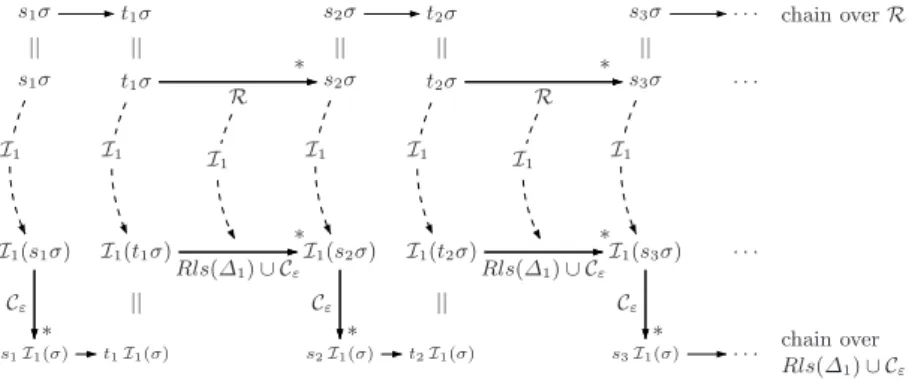
[24, 29] and in the original proofs of Gramlich [16], we map anyR-reduction to a reduction w.r.t.Rls(∆1)∪Cε. However, our mappingI1is a modification of these earlier mappings, since terms g(t1, . . . , tn) with g /∈ ∆1 are treated differently.
Fig. 1 illustrates that by this mapping, every minimal chain overRcorresponds to a chain overRls(∆1)∪Cε, but instead of the substitutionσone uses a different substitutionI1(σ). Thus, the observation (9) also holds for∆1instead of∆0.
chain overR
chain over Rls(∆1)∪ Cε s1σ
s1σ
I1(s1σ)
s1I1(σ) I1
||
* Cε
t1σ
t1σ
I1(t1σ)
t1I1(σ)
||
||
I1 I1
s2σ
s2σ
I1(s2σ)
s2I1(σ) I1
||
* Cε
* R
* Rls(∆1)∪ Cε
t2σ
t2σ
I1(t2σ)
t2I1(σ)
||
||
I1 I1
s3σ
s3σ
I1(s3σ)
s3I1(σ) I1
||
* Cε
* R
* Rls(∆1)∪ Cε
. . .
. . .
. . .
. . .
Fig. 1.Transformation of chains
Intuitively,I1(t) “collects” all terms thatt can be reduced to. However, we only regard reductions on or below symbols that are not from∆1. Normal forms whose roots are not from∆1may be replaced by a fresh variable. To represent a collectiont1, . . . , tn of terms by just one term, one uses c(t1,c(t2, ...c(tn, x)...)).
Definition 14. Let∆⊆ F ∪F♯and lett∈ T(F ∪F♯,V)be a terminating term.
We define I1(t):
I1(x) =x for x∈ V
I1(f(t1, ..., tn)) =f(I1(t1), ...,I1(tn)) for f ∈∆ I1(g(t1, ..., tn)) =Comp({g(I1(t1), ...,I1(tn))} ∪ Red1(g(t1, ..., tn))) for g /∈∆ whereRed1(t) ={I1(t′)|t→R t′}. Moreover,Comp({t} ⊎M) =c(t,Comp(M)) and Comp(∅) =xnew, where xnew is a fresh variable. To ensure thatComp is well-defined we assume that in the recursive definition of Comp({t} ⊎M), t is smaller than all terms inM due to some total well-founded order>T on terms.
For every terminating substitutionσ(i.e.,σ(x)is terminating for allx∈ V), we define the substitutionI1(σ)asI1(σ) (x) =I1(σ(x))for all x∈ V.
Note that Def. 14 is only possible for terminating termst, since otherwise, I1(t) could be infinite. Before we can show that Thm. 11 can be adapted to the refined definition ∆1, we need some additional properties of Comp and I1. In contrast to the corresponding lemmas in [24, 29], they demonstrate that the rules
of∆0\∆1are not needed and we show in Lemma 16 (ii) and (iii) how to handle dependency pairs and rules where the left-hand side is not fromT(∆1,V).8 Lemma 15 (Properties of Comp). If t∈M thenComp(M)→+Cε t.
Proof. For t1 <T · · · <T tn and any 1 ≤i ≤nwe have Comp({t1, . . . , tn}) = c(t1, . . .c(ti, . . .c(tn, x). . .). . .)→∗Cεc(ti, . . .c(tn, x). . .)→Cεti. ⊓⊔ Lemma 16 (Properties of I1). Let ∆ ⊆ F ∪ F♯ where f ∈ ∆ and f ❂1 g implies g ∈∆. Let t, s, tσ∈ T(F ∪ F♯,V)be terminating terms and let σ be a terminating substitution.
(i) Ift∈ T(∆,V)thenI1(tσ) =tI1(σ).
(ii) I1(tσ)→∗Cε tI1(σ).
(iii) Ift→{l→r}s by a root reduction step wherel→r∈ Randroot(l)∈∆, then I1(t)→+{l→r}∪Cε I1(s).
(iv) Ift→Rswith root(t)6∈∆, then I1(t)→+Cε I1(s).
(v) Ift→{l→r}s wherel→r∈ R,
then I1(t)→+{l→r}∪Cε I1(s) ifroot(l)∈∆ andI1(t)→+Cε I1(s)otherwise.
Proof.
(i) The proof is a straightforward structural induction ont.
(ii) The proof is by structural induction on t. The only interesting case is t= g(t1, . . . , tn) whereg /∈∆. Then we obtain
I1(g(t1, ..., tn)σ) = Comp({g(I1(t1σ), ...,I1(tnσ))} ∪ Red1(g(t1σ, . . . , tnσ)))
→+Cε g(I1(t1σ), ...,I1(tnσ)) by Lemma 15
→∗Cε g(t1I1(σ), . . . , tnI1(σ)) by induction hypothesis
= g(t1, . . . , tn)I1(σ)
(iii) We havet=lσ→Rrσ=s. By the definition of❂1,ris a term ofT(∆,V).
Using (ii) and (i) we getI1(lσ)→∗CεlI1(σ)→{l→r}rI1(σ) =I1(rσ).
(iv) follows byI1(t) =Comp({. . .} ∪ Red1(t)),I1(s)∈ Red1(t), and Lemma 15.
(v) We do induction on the position p of the redex. If root(t) ∈/ ∆, we use (iv). If root(t)∈∆ andpis the root position, we apply (iii). Otherwise,p is below the root, t=f(t1, . . . , ti, . . . , tn),s=f(t1, . . . , si, . . . , tn),f ∈∆, andti→{l→r}si. Then the claim follows from the induction hypothesis. ⊓⊔ Now we show that in Thm. 11 one may replace∆0 by∆1.
Theorem 17 (Improved Modular Termination, Version 1). A TRSRis terminating if for every cycleP of the dependency graph there is aCε-compatible reduction pair (%,≻) and an argument filtering π satisfying both constraint Thm. 7 (a) and
(b) l%πr for all rulesl→r∈Rls(∆1(P,R))
8 Here, equalities in the lemmas of [24, 29] are replaced by Cε-steps. This is possible by including the termg(I1(t1), . . . ,I1(tn)) in the definition ofI1(g(t1, ..., tn)).
Proof. The proof is as for Thm. 11, but instead of (9) one uses this observation:
Every minimalP-chain overRis aP-chain overRls(∆1(P,R))∪ Cε. (10) To prove (10), let s1 →t1, s2 → t2, . . . be a minimal P-chain overR. Hence, there is a substitutionσsuch that tiσ→∗Rsi+1σ and all termssiσandtiσare terminating. This enables us to applyI1to bothtiσandsiσ(where we choose∆ to be∆1(P,R)). Using Lemma 16 (v) we obtainI1(tiσ)→∗Rls(∆1)∪CεI1(si+1σ).
Moreover, by the definition of❂1, alltiare terms over the signature∆1. Thus, by Lemma 16 (i) and (ii) we get tiI1(σ) =I1(tiσ)→∗Rls(∆1)∪Cε I1(si+1σ)→∗Cε si+1I1(σ) stating thats1→t1, s2→t2, . . . is also a chain overRls(∆1)∪Cε. ⊓⊔
4 Dependences With Respect to Argument Filterings
For innermost termination, one may first apply the argument filteringπand de- termine the usable rulesU(P, π) afterwards, cf. [12]. The advantage is that the argument filtering may eliminate some symbols f from right-hand sides of de- pendency pairs and rules. Then, thef-rules do not have to be weakly decreasing anymore. We also presented an algorithm to determine suitable argument filter- ings, which is non-trivial since the filtering determines the resulting constraints.
We now introduce a corresponding improvement for termination by defining
“dependence” w.r.t. an argument filtering. Then a cycle only depends on those symbols that are not dropped by the filtering. However, this approach is only sound for non-collapsing argument filterings. Consider the non-terminating TRS f(s(x))→f(double(x)) double(0)→0 double(s(x))→s(s(double(x))) In the cycle {F(s(x)) → F(double(x))}, the filtering π(double) = 1 results in {F(s(x)) → F(x)}. Since the filtered pair has no defined symbols, we would conclude that no rule must be weakly decreasing for this cycle. But then we can solve the cycle’s only constraintF(s(x))≻F(x) and falsely prove termination.9 Example 18. We extend the TRS of Ex. 12 by rules for prime numbers.
prime(s(s(x)))→pr(s(s(x)),s(x)) pr(x,s(0))→true
eq(0,0)→true pr(x,s(s(y)))→if(divides(s(s(y)), x), x,s(y)) eq(s(x),0)→false if(true, x, y)→false
eq(0,s(y))→false if(false, x, y)→pr(x, y)
eq(s(x),s(y))→eq(x, y) divides(y, x)→eq(x,times(div(x, y), y)) The cycle{PR(x,s(s(y)))→IF(divides(s(s(y)), x), x,s(y)),IF(false, x, y)→PR(x, y)} depends ondivides and hence, on divand times. So for this cycle, Thm. 17
9 Essentially, we prove absence of infiniteπ(P)-chains overπ(R). But ifπis collapsing, then the rules ofπ(R) may have left-hand sideslwith root(l)∈ C orl∈ V. Thus, inspecting the defined symbols in a termπ(t) is not sufficient to estimate which rules may be used for theπ(R)-reduction ofπ(t).
requires thediv- andtimes-rules to be weakly decreasing. This is impossible with reduction pairs based on RPOS, KBO, or polynomial orders, cf. Ex. 12.
But if we first use the filteringπ(IF) = [2,3] and compute dependences after- wards, then the cycle no longer depends ondivides,div, ortimes. If one modifies
“dependence” in this way, then the constraints can again be solved by LPO.
Definition 19 (Refined Dependence, Version 2).Letπbe a non-collapsing argument filtering. For two function symbols f and g we define f ❂2g iff there is a rule l → r∈ Rls({f}) where g occurs in π(r). For a cycle of dependency pairs P, we defineP ❂2g iff there is a pairs→t∈ P where g occurs inπ(t).
We define ∆2(P,R, π) ={f | P ❂+2 f} and omitP,R,πif they are clear from the context.
To show that∆1may be replaced by∆2in Thm.17, we define a new mappingI2. Definition 20. Let π be a non-collapsing argument filtering, ∆⊆ F ∪ F♯,t∈ T(F ∪F♯,V)be terminating. We defineI2(t). Here,Red2(t) ={I2(t′)|t→Rt′}.
I2(x) =x for x∈ V
I2(f(t1, . . . , tn)) =f(I2(ti1), . . . ,I2(tik)) for f ∈∆, π(f) = [i1, ..., ik] I2(g(t1, . . . , tn)) =Comp({g(I2(ti1), . . . ,I2(tik))}
∪ Red2(g(t1, . . . , tn)) ) for g /∈∆,π(g) = [i1, ..., ik] Lemma 21 differs from the earlier Lemma 16, since I2 already applies the argument filteringπ and in (v), we have “∗” instead of “+”, as a reduction on a position that is filtered away leads to the same transformed terms w.r.t.I2. Lemma 21 (Properties of I2). Let π be a non-collapsing argument filtering and let ∆ ⊆ F ∪ F♯ such that f ∈ ∆ and f ❂2 g implies g ∈∆. Lett, s, tσ ∈ T(F ∪ F♯,V)be terminating and letσ be a terminating substitution.
(i) Ifπ(t)∈ T(∆π,V)thenI2(tσ) =π(t)I2(σ).
(ii) I2(tσ)→∗Cε π(t)I2(σ).
(iii) Ift→{l→r}s by a root reduction step wherel→r∈ Randroot(l)∈∆, then I2(t)→+{π(l)→π(r)}∪CεI2(s).
(iv) Ift→Rswith root(t)6∈∆, then I2(t)→+Cε I2(s).
(v) Ift→{l→r}s wherel→r∈ R, then
I2(t)→∗{π(l)→π(r)}∪Cε I2(s) ifroot(l)∈∆ andI2(t)→∗Cε I2(s) otherwise.
Proof. The proof is analogous to the proof of Lemma 16. ⊓⊔ We are restricted to non-collapsing filterings when determining the rules that have to be weakly decreasing. But one can still use arbitrary (possibly collapsing) filterings in the dependency pair approach. For every filtering π we define its non-collapsing variant π′ asπ′(f) =π(f) ifπ(f) = [i1, . . . , ik] andπ′(f) = [i] if π(f) =i. Now we show that in Thm. 17 one may replace∆1 by∆2.
Theorem 22 (Improved Modular Termination, Version 2). A TRSRis terminating if for every cycleP of the dependency graph there is aCε-compatible reduction pair (%,≻) and an argument filtering π satisfying both constraint Thm. 7 (a) and
(b) l%πr for l→r∈Rls(∆2(P,R, π′)), where π′ isπ’s non-collapsing variant Proof. Instead of (10), now we need the following main observation for the proof.
If s1 → t1, s2 → t2, . . . is a minimal P-chain over R, then π′(s1) → π′(t1), π′(s2)→π′(t2), . . . is aπ′(P)-chain overπ′(Rls(∆2(P,R, π′)))∪Cε. (11) Similar to the proof of (10), tiσ →∗R si+1σ implies that π′(ti)I2(σ) = I2(tiσ)
→∗π′(Rls(∆2))∪Cε I2(si+1σ) →∗Cε π′(si+1)I2(σ) by Lemma 21 (i), (v), and (ii), which proves (11).
To show that (11) implies Thm. 22, assume that s1 → t1, s2 →t2, . . . is a minimal infinite P-chain overR. Then by (11) there is a substitution δ(I2(σ) from above) withπ′(ti)δ→∗π′(Rls(∆2))∪Cε π′(si+1)δfor alli. Letπ′′be the argu- ment filtering for the signatureFπ′∪Fπ♯′ which only performs the collapsing steps ofπ(i.e., ifπ(f) =iand thusπ′(f) = [i], we haveπ′′(f) = 1). All other symbols of Fπ′ ∪ Fπ♯′ are not filtered by π′′. Hence, π= π′′◦π′. We extend π′′ to the new symbolcby definingπ′′(c) = [1,2]. Hence,Cε-compatibility of%impliesCε- compatibility of%π′′. Constraint (b) requiresπ(l)%π(r) for all rules ofRls(∆2).
Therefore, we haveπ′(l)%π′′ π′(r), and thus, all rules of π′(Rls(∆2))∪ Cε are decreasing w.r.t.%π′′. This impliesπ′(ti)δ%π′′ π′(si+1)δfor alli. Moreover, (a) impliesπ′(si)δ≻π′′π′(ti)δfor infinitely manyiandπ′(si)δ%π′′π′(ti)δfor all remainingi. This contradicts the well-foundedness of≻π′′. ⊓⊔ Now we are nearly as powerful as for innermost termination. The only differ- ence between ∆2(P,R, π) and U(P, π) is thatU(P, π) may disregard subterms of right-hand sides of dependency pairs if they also occur on the left-hand side [12], since they are instantiated to normal forms in innermost chains. But for the special case of constructor systems, the left-hand sides of dependency pairs are constructor terms and thus∆2(P,R, π) =U(P, π). The other differences be- tween termination and innermost termination are that the innermost dependency graph is a subgraph of the dependency graph and may have fewer cycles. More- over, the conditions for applying dependency pair transformations by narrowing, rewriting, or instantiation [2, 10, 12] are less restrictive for innermost termina- tion. Finally for termination, we useCε-compatible reduction pairs, which is not necessary for innermost termination. However, virtually all reduction pairs used in practice areCε-compatible. So in general, innermost termination is still easier to prove than termination, but the difference has become much smaller.
5 Removing Rules
To reduce the constraints for termination proofs even further, in this section we present a technique to remove rules of the TRS that are not relevant for termination. To this end, the constraints for a cycle P may be pre-processed with a reduction pair (%,≻). If all dependency pairs of P and all rules that P depends on are at least weakly decreasing (w.r.t. %), then one may remove
all those rules R≻ that are strictly decreasing (w.r.t.≻). So instead of proving absence of infiniteP-chains overRone only has to regardP-chains overR \ R≻. In contrast to related approaches to remove rules [15, 23, 30], we permit arbi- trary reduction pairs and remove rules in the modular framework of dependency pairs instead of pre-processing a full TRS. So when removing rules for a cycleP, we only have to regard the rulesP depends on. Moreover, removing rules can be done repeatedly with different reduction pairs (%,≻). Thm. 23 can also be adap- ted for innermost termination proofs with similar advantages as for termination.
Theorem 23 (Modular Removal of Rules).LetP be a set of pairs,Rbe a TRS, and (%,≻)be a reduction pair where ≻ is monotonic and Cε-compatible.
If l(%)r for all l → r ∈Rls(∆1(P,R)) and s(%)t for all s→ t ∈ P then the absence of minimal infiniteP-chains overR\R≻implies the absence of minimal infinite P-chains overRwhere R≻={l→r∈Rls(∆1(P,R))|l≻r}.10 Proof. Lets1 →t1, s2→t2, . . . be an infinite minimal P-chain overR. Hence, tiσ →∗R si+1σ. We show that in these reductions, R≻-rules are only applied for finitely many i. Sotiσ→∗R\R≻ si+1σ for all i≥ n for some n∈ IN. Thus, sn → tn, sn+1 → tn+1, . . . is a minimal infinite P-chain over R \ R≻ which proves Thm. 23.
Assume thatR≻-rules are applied for infinitely many i. By Lemma 16 (v) we get I1(tiσ) →∗Rls(∆1)∪Cε I1(si+1σ). As ≻ is Cε-compatible and →Rls(∆1)⊆
(%), we have I1(tiσ)(%)I1(si+1σ). Moreover, whenever an R≻-rule is used in tiσ→∗R si+1σ, then by Lemma 16 (v), the same rule or at least one Cε-rule is used in the reduction fromI1(tiσ) toI1(si+1σ). (This would not hold forI2, cf.
Lemma 21 (v).) Thus, then we have I1(tiσ)≻ I1(si+1σ) since≻is monotonic.
As R≻-reductions are used for infinitely many i, we haveI1(tiσ) ≻ I1(si+1σ) for infinitely manyi. Using Lemma 16 (ii), (i), and s(%)t for all pairs inP, we obtainI1(siσ)→∗Cε siI1(σ)(%)tiI1(σ) =I1(tiσ). By Cε-compatibility of ≻, we getI1(siσ)(%)I1(tiσ) for alli. This contradicts the well-foundedness of≻. ⊓⊔ Rule removal has three benefits. First, the rulesR≻do not have to be weakly decreasing anymore after the removal. Second, the rules thatR≻depends on do not necessarily have to be weakly decreasing anymore either. More precisely, since we only regard chains over R \ R≻, only the rules in ∆1(P,R \ R≻) or
∆2(P,R \ R≻, . . .) must be weakly decreasing. And third, it can happen thatP is not a cycle anymore. Then no constraints at all have to be built forP. More precisely, we can delete all edges in the dependency graph between pairss→t andu→v ofP where s→t,u→v is anR-chain, but not anR \ R≻-chain.
Example 24. We extend the TRS of Ex. 18 by the following rules.
p(s(x))→x plus(s(x), y)→s(plus(p(s(x)), y)) plus(x,s(y))→s(plus(x,p(s(y))))
10Using∆2instead of∆1makes Thm. 23 unsound. Consider{f(a,b)→f(a,a),a→b}.
Withπ(F) = [1], an LPO-reduction pair makes the filtered dependency pair weakly decreasing and the rule strictly decreasing (F(a)%F(a) anda≻b). But then Thm.
23 would state that we can remove the rule and only prove absence of infinite chains ofF(a,b)→F(a,a) over the empty TRS. Then we could falsely prove termination.
For the cycle{PLUS(s(x), y) →PLUS(p(s(x)), y),PLUS(x,s(y))→PLUS(x, p(s(y)))} there is no argument filtering and reduction pair (%,≻) with a quasi- simplification order%satisfying the constraints of Thm. 22. The reason is that due top’s rule, the filtering cannot drop the argument ofp. Soπ(PLUS(p(s(x)), y)) % π(PLUS(s(x), y)) and π(PLUS(x,p(s(y)))) % π(PLUS(x,s(y))) hold for any quasi-simplification order%. Furthermore, the transformation technique of
“narrowing dependency pairs” [2, 10, 12] is not applicable, since the right-hand side of each dependency pair above unifies with the left-hand side of the other dependency pair. Therefore, automated tools based on dependency pairs fail.
In contrast, by Thm. 23 and a reduction pair with the polynomial interpreta- tionPol(PLUS(x, y)) =x+y,Pol(s(x)) =x+1,Pol(p(x)) =x,p’s rule is strictly decreasing and can be removed. Then,pis a constructor. If one uses the technique of “instantiating dependency pairs” [10, 12], for this cycle the second dependency pair can be replaced byPLUS(p(s(x)),s(y))→PLUS(p(s(x)),p(s(y))). Now the two pairs form no cycle anymore and thus, no constraints at all are generated.
If we also add the rulep(0)→0, then againp(s(x))→xcan be removed by Thm. 23 but pdoes not become a constructor and we cannot delete the whole cycle. Still, the resulting constraints are satisfied by an argument filtering with π(PLUS) = [1,2],π(s) =π(p) = [ ] and an LPO with the precedences>p>0.
Note that here, it is essential that Thm. 23 only requiresl%rfor rulesl→r that P depends on. In contrast, previous techniques [15, 23, 30] would demand that all rules including the ones for div and times would have to be at least weakly decreasing. As shown in Ex. 12, this is impossible with standard orders.
To automate Thm. 23, we use reduction pairs (%,≻) based on linear polyno- mial interpretations with coefficients from {0,1}. Since≻must be monotonic, n-ary function symbols can only be mapped toPn
i=1xi or to 1 +Pn
i=1xi. Thus, there are only two possible interpretations resulting in a small search space.
Moreover, polynomial orders can solve constraints where one inequality must be strictly decreasing and all others must be weakly decreasing in just one search attempt without backtracking [13]. In this way, Thm. 23 can be applied very efficiently. Since removing rules never complicates termination proofs, Thm. 23 should be applied repeatedly as long as some rule is deleted in each application.
Note that whenever a dependency pair (instead of a rule) is strictly decreas- ing, one has solved the constraints of Thm. 17 and can delete the cycle. Thus, one should not distinguish between rule- and dependency pair-constraints when applying Thm. 23 and just search for a strict decrease in any of the constraints.
6 Conclusion and Empirical Results
We presented new results to reduce the constraints for termination proofs with dependency pairs substantially. By Sect. 3 and 4, it suffices to require weak de- crease of the dependent rules, which correspond to the usable rules regarded for innermost termination. So surprisingly, the constraints for termination and in- nermost termination are (almost) the same. Moreover, we showed in Sect. 5 that
one may pre-process the constraints for each cycle and eliminate rules that are strictly decreasing. All our results can also be used together with dependency pair transformations [2, 10, 12] which often simplify (innermost) termination proofs.
We implemented our results in the systemAProVE11[14] and tested it on the 130 terminating TRSs from [3, 8, 25]. The following table gives the percentage of the examples where termination could be proved within a timeout of 30 s and the time for running the system on all examples (including the ones where the proof failed). Our experiments were performed on a Pentium IV with 2.4 GHz and 1 GB memory. We used reduction pairs based on the embedding order, LPO, and linear polynomial interpretations with coefficients from{0,1}(“Polo”). The table shows that with every refinement from Thm. 7 to Thm. 22, termination proving becomes more powerful and for more complex orders than embedding, efficiency also increases considerably. Moreover, a pre-processing with Thm. 23 using “Polo” makes the approach even more powerful. Finally, if one also uses dependency pair transformations (“tr”), one can increase power further. To mea- sure the effect of our contributions, in the first 3 rows we did not use the tech- nique for innermost termination proofs, even if the TRS is non-overlapping. (If one applies the innermost termination technique in these examples, we can prove termination of 95 % of the examples in 23 s with “Polo”.) Finally, in the last row (“Inn”) we verifiedinnermost termination with “Polo” and usable rulesU(P) as in Thm. 17, with usable rulesU(P, π) as in Thm. 22, with a pre-processing as in Thm. 23, and with dependency pair transformations. This row demonstrates that termination is now almost as easy to prove as innermost termination. To summarize, our experiments show that the contributions of this paper are in- deed relevant and successful in practice, since the reduction of constraints makes automated termination proving significantly more powerful and faster.
Thm. 7 Thm. 11 Thm. 17 Thm. 22 Thm. 22, 23 Thm. 22, 23, tr Emb 39 s, 28 % 7 s, 30 % 42 s, 38 % 50 s, 52 % 51 s, 65 % 82 s, 78 % LPO 606 s, 51 % 569 s, 54 % 261 s, 59 % 229 s, 61 % 234 s, 75 % 256 s, 84 % Polo 9 s, 61 % 8 s, 66 % 5 s, 73 % 5 s, 78 % 6 s, 85 % 9 s, 91 %
Inn 8 s, 78 % 8 s, 82 % 10 s, 88 % 31 s, 97 %
References
1. T. Arts. System description: The dependency pair method. In L. Bachmair, editor, Proc. 11th RTA, LNCS 1833, pages 261–264, Norwich, UK, 2000.
2. T. Arts and J. Giesl. Termination of term rewriting using dependency pairs. The- oretical Computer Science, 236:133–178, 2000.
3. T. Arts and J. Giesl. A collection of examples for termination of term rewriting using dependency pairs. Technical Report AIB-2001-0912, RWTH Aachen, 2001.
4. F. Baader and T. Nipkow. Term Rewriting and All That. Cambridge, 1998.
5. C. Borralleras, M. Ferreira, and A. Rubio. Complete monotonic semantic path orderings. In D. McAllester, editor,Proc. 17th CADE, LNAI 1831, pages 346–364, Pittsburgh, PA, USA, 2000.
11http://www-i2.informatik.rwth-aachen.de/AProVE. Our contributions are inte- grated inAProVE 1.1-beta, which does not yet contain all options ofAProVE 1.0.
6. E. Contejean, C. March´e, B. Monate, and X. Urbain.CiME.http://cime.lri.fr.
7. N. Dershowitz. Termination of rewriting. J. Symb. Comp., 3:69–116, 1987.
8. N. Dershowitz. 33 examples of termination. In Proc. French Spring School of Theoretical Computer Science, LNCS 909, pages 16–26, Font Romeux, 1995.
9. O. Fissore, I. Gnaedig, and H. Kirchner. Cariboo: An induction based proof tool for termination with strategies. In C. Kirchner, editor, Proc. 4th PPDP, pages 62–73, Pittsburgh, PA, USA, 2002. ACM Press.
10. J. Giesl and T. Arts. Verification of Erlang processes by dependency pairs. Appl.
Algebra in Engineering, Communication and Computing, 12(1,2):39–72, 2001.
11. J. Giesl, T. Arts, and E. Ohlebusch. Modular termination proofs for rewriting using dependency pairs. Journal of Symbolic Computation, 34(1):21–58, 2002.
12. J. Giesl, R. Thiemann, P. Schneider-Kamp, and S. Falke. Improving dependency pairs. In Vardi and Voronkov, editors,Proc 10th LPAR, LNAI 2850, 165–179, 2003.
13. J. Giesl, R. Thiemann, P. Schneider-Kamp, and S. Falke. Mechanizing dependency pairs. Technical Report AIB-2003-0812, RWTH Aachen, Germany, 2003.
14. J. Giesl, R. Thiemann, P. Schneider-Kamp, and S. Falke. Automated termination proofs withAProVE. In v. Oostrom, editor,Proc. 15th RTA, LNCS, Aachen, 2004.
15. J. Giesl and H. Zantema. Liveness in rewriting. In R. Nieuwenhuis, editor,Proc.
14th RTA, LNCS 2706, pages 321–336, Valencia, Spain, 2003.
16. B. Gramlich. Generalized sufficient conditions for modular termination of rewrit- ing.Appl. Algebra in Engineering, Communication & Computing, 5:131–158, 1994.
17. B. Gramlich. Abstract relations between restricted termination and confluence properties of rewrite systems. Fundamenta Informaticae, 24:3–23, 1995.
18. N. Hirokawa and A. Middeldorp. Automating the dependency pair method. In F. Baader, editor,Proc. 19th CADE, LNAI 2741, Miami Beach, FL, USA, 2003.
19. N. Hirokawa and A. Middeldorp. Tsukuba termination tool. In R. Nieuwenhuis, editor,Proc. 14th RTA, LNCS 2706, pages 311–320, Valencia, Spain, 2003.
20. S. Kamin and J. J. L´evy. Two generalizations of the recursive path ordering.
Unpublished Manuscript, University of Illinois, IL, USA, 1980.
21. D. Knuth and P. Bendix. Simple word problems in universal algebras. In J. Leech, editor,Computational Problems in Abstract Algebra, pages 263–297. 1970.
22. K. Kusakari, M. Nakamura, and Y. Toyama. Argument filtering transformation.
In G. Nadathur, editor,Proc. 1st PPDP, LNCS 1702, pages 48–62, Paris, 1999.
23. D. Lankford. On proving term rewriting systems are Noetherian. Technical Report MTP-3, Louisiana Technical University, Ruston, LA, USA, 1979.
24. E. Ohlebusch. Advanced Topics in Term Rewriting. Springer, 2002.
25. J. Steinbach. Automatic termination proofs with transformation orderings. In J. Hsiang, editor,Proc. 6th RTA, LNCS 914, pages 11–25, Kaiserslautern, Germany, 1995. Full version in Technical Report SR-92-23, Universit¨at Kaiserslautern.
26. J. Steinbach. Simplification orderings: History of results. Fund. I., 24:47–87, 1995.
27. R. Thiemann and J. Giesl. Size-change termination for term rewriting. In R. Nieu- wenhuis, editor,Proc. 14th RTA, LNCS 2706, pages 264–278, Valencia, Spain, 2003.
28. Y. Toyama. Counterexamples to the termination for the direct sum of term rewrit- ing systems. Information Processing Letters, 25:141–143, 1987.
29. X. Urbain. Automated incremental termination proofs for hierarchically defined term rewriting systems. In R. Gor´e, A. Leitsch, and T. Nipkow, editors, Proc.
IJCAR 2001, LNAI 2083, pages 485–498, Siena, Italy, 2001.
30. H. Zantema.TORPA: Termination of rewriting proved automatically. InProc. 15th RTA, LNCS, Aachen, 2004. Full version in TU/e CS-Report 03-14, TU Eindhoven.
12Available fromhttp://aib.informatik.rwth-aachen.de