Noname manuscript No.
(will be inserted by the editor)
Analyzing Innermost Runtime Complexity of Term Rewriting by Dependency Pairs
Lars Noschinski · Fabian Emmes · J ¨urgen Giesl
the date of receipt and acceptance should be inserted later
Abstract We present a modular framework to analyze the innermost runtime complexity of term rewrite systems automatically. Our method is based on the dependency pair framework for termination analysis. In contrast to previous work, we developed adirectadaptation of successful termination techniques from the dependency pair framework in order to use them for complexity analysis. By extensive experimental results, we demonstrate the power of our method compared to existing techniques.
1 Introduction
In practice, one is often not only interested in analyzing the termination of programs, but one also wants to check whether algorithms terminate inreasonable(e.g., polynomial)time.
While termination of term rewrite systems (TRSs) is well studied, only recently first results were obtained which adapt termination techniques in order to obtain polynomial complexity bounds automatically, e.g., [2–5,7,10,17–19,22–24,26,29,30]. Here, [3,17–19] consider the dependency pair (DP) method[1, 11, 12, 16], which is one of the most popular termination techniques for TRSs. Moreover, [30] introduces a similar modular approach for complexity analysis based on relative rewriting. There is also a related area ofimplicit computational complexitywhich aims at characterizing complexity classes, e.g., using type systems [21], bottom-up logic programs [15], and also using termination techniques like dependency pairs (e.g., [23]).
Techniques for automated termination analysis of term rewriting are very powerful and have been successfully used to analyze termination of programs in many different languages (e.g.,Java [8, 28], Haskell[13], and Prolog[14]). Hence, by adapting these termination techniques, the ultimate goal is to obtain approaches which can also analyze the complexity of programs automatically.
Supported by the DFG grant GI 274/5-3.
Lars Noschinski
Institut f¨ur Informatik, TU Munich, Germany Fabian Emmes·J¨urgen Giesl
LuFG Informatik 2, RWTH Aachen University, Germany
In this paper, we present a fresh adaptation of the DP framework forinnermost runtime complexity analysis[17]. We use a different notion of “dependency pairs” for complexity analysis than previous works [3, 17, 19]. This allows us to adapt the termination techniques (“processors”) of the DP framework in a much more direct way when using them for com- plexity analysis. On the other hand, our approach is restricted to theinnermostevaluation strategy, whereas [3, 17, 19] also analyze runtime complexity of full rewriting. Like [30], our method is modular (i.e., we can determine the complexity of a TRS by determining the complexity of certain sub-problems and by returning the maximum of these complexi- ties). But in contrast to [30], which allows to investigatederivational complexity[20], we focus on innermost runtime complexity. In this way, we can inherit the modularity aspects of the DP framework and benefit from its transformation techniques, which increases power significantly.
A preliminary version of this paper appeared in [27]. The current paper extends [27]
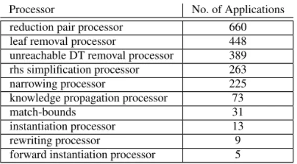
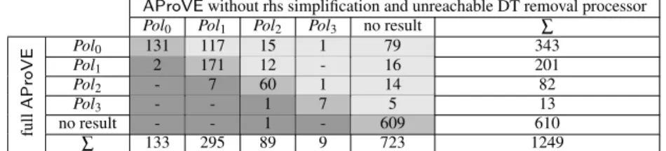
substantially, e.g., by including proofs for all theorems, by two new processors for com- plexity analysis (Thm. 32 and 34) and experiments to justify their significance, by detailed information on the impact of the different processors in Sect. 6, and by several additional remarks throughout the paper.
After introducing preliminaries in Sect. 2, in Sect. 3 we adapt the concept of depen- dency pairsfrom termination analysis to so-calleddependency tuplesfor complexity analy- sis. While theDP frameworkfor termination works onDP problems, we now work onDT problems(Sect. 4). Sect. 5 adapts the processors of the DP framework in order to analyze the complexity of DT problems. We implemented our contributions in the termination analyzer AProVE. Due to the results of this paper,AProVEwas the most powerful tool for innermost runtime complexity analysis in theInternational Termination Competitionin 2010 – 2012.
In Sect. 6 we report on extensive experiments where we compared our technique empirically with previous approaches.
2 Runtime Complexity of Term Rewriting
See e.g. [6] for the basics of term rewriting, where we only consider finite rewrite systems.
LetT(Σ,V)be the set of all terms over a (finite) signatureΣand a set of variablesV. We just writeT ifΣandVare clear from the context. Thearityof a function symbolf∈Σis denoted by ar(f)and the size of a term is|x|=1 forx∈Vand|f(t1, . . . ,tn)|=1+|t1|+. . .+|tn|.
Thederivation heightof a termtw.r.t. a relation→is the length of the longest sequence of
→-steps starting witht, i.e., dh(t,→) =sup{n| ∃t0∈T,t→nt0}, cf. [20].
Here, for any setM⊆N∪ {ω}, “supM” is the least upper bound ofMand sup∅=0.
Note that since we restricted ourselves to finite TRSs, the rewrite relation is finitely branch- ing and thus, the set{n| ∃t0∈T,t→nt0}is infinite ifftstarts an infinitely long sequence of→-steps. Thus, dh(t,→) =ωifftis non-terminating w.r.t. the relation→(i.e., iff there is an infinite reductiont→t1→t2→. . .). Note that in the literature, dh is usually left unde- fined for terms with non-terminating derivations. However, we extended it in order to treat terminating and non-terminating terms in a uniform way.
Example 1 As an example, consider the TRSR={dbl(0)→0,dbl(s(x))→s(s(dbl(x)))}.
Thendh(dbl(sn(0)),→R) =n+1, butdh(dbln(s(0)),→R) =2n+n−1.
For a TRSRwithdefined symbolsΣd(R) ={root(`)|`→r∈R}, a termf(t1, . . . ,tn)is basiciff∈Σd(R)andt1, . . . ,tndo not contain symbols fromΣd(R). IfRis clear from the context, we just writeΣdinstead ofΣd(R). So forRin Ex. 1, the basic terms aredbl(sn(0))
anddbl(sn(x))forn∈N,x∈V. Theinnermost runtime complexity functionircRmaps any n∈N to the length of a longest sequence of→i R-steps starting with a basic termt with
|t| ≤n. Here, “→i R” is the innermost rewrite relation andTBis the set of all basic terms.
Definition 2 (ircR[17])For a TRSR, itsinnermost runtime complexity functionircR:N→ N∪{ω}is ircR(n) =sup{dh(t,→i R)|t∈TB,|t| ≤n}.
If one only considers evaluations of basic terms, the (runtime) complexity of the TRS Rin Ex. 1 is linear (ircR(n) =n−1 forn≥2). But if one also permits evaluations starting withdbln(s(0)), the complexity of thedbl-TRS is exponential.
When analyzing the complexity ofprograms, one is typically interested in evaluations where a defined function likedblis applied to data objects (i.e., terms without defined sym- bols). Therefore,runtime complexitycorresponds to the usual notion of “complexity” for programs [4, 5]. Note that most termination techniques which transform programs to TRSs (e.g., [8, 13, 14, 28]) result in rewrite systems where one only regards innermost rewrite se- quences. This also holds for techniques to analyze termination of languages likeHaskellby term rewriting [13], althoughHaskellhas a lazy (outermost) evaluation strategy. Thus, we restrict ourselves to innermost rewriting, since this suffices to analyze TRSs resulting from the transformation of programs. So for any TRSR, we want to determine theasymptotic complexityof the function ircR.
Definition 3 (Asymptotic Complexities)LetC={Pol0,Pol1,Pol2, . . . ,?}with the order Pol0<Pol1 <Pol2 <. . .< ?. Let v be the reflexive closure of <. For any function f :N→N∪ {ω} we define itscomplexity ι(f)∈C as follows:ι(f) =Polk ifk is the smallest number with f(n)∈O(nk)andι(f) =? if there is no suchk. For any TRSR, we define itscomplexityιRasι(ircR).
So the TRS R in Ex. 1 has linear complexity, i.e.,ιR=Pol1. As another example, consider the following TRSRwhere “m” stands for “minus”.
Example 4 m(x,y)→if(gt(x,y),x,y) gt(0,k)→false p(0)→0
if(true,x,y)→s(m(p(x),y)) gt(s(n),0)→true p(s(n))→n
if(false,x,y)→0 gt(s(n),s(k))→gt(n,k) Here,ιR=Pol2(e.g.,m(sn(0),sk(0))starts evaluations of quadratic length).
In Def. 3, we restricted ourselves to polynomial complexity classes, because the under- lying techniques that we use to generate suitable well-founded orders automatically result in polynomial bounds. However, the approach could also be used for other complexity classes (then the order<would have to be extended accordingly).
3 Dependency Tuples
In the DP method, for every f ∈Σdone introduces a fresh symbol f]with ar(f) =ar(f]).
For a termt = f(t1, . . . ,tn) with f ∈Σd we definet]= f](t1, . . . ,tn)and let T]={t] | t∈T,root(t)∈Σd}. LetPos(t)contain all positions oftand letPosd(t) ={π|π∈Pos(t), root(t|π)∈Σd}. Then for every rule`→rwithPosd(r) ={π1, . . . ,πn}, itsdependency pairs are`]→r|]π
1, . . . ,`]→r|]πn.
While DPs are used for termination, for complexity we have to regardalldefined func- tions in a right-hand sideat once. The reason is that in order to estimate the derivation
height of a term corresponding to the left-hand side of a rule`→r, we have to consider the rewrite steps originating fromr. Here, all subterms ofrwith defined root symbol may pos- sibly be reduced and can thus contribute to the overall derivation height. Thus, we extend the concept ofweak dependency pairs[17–19] and only build a singledependency tuple
`]→[r|]π1, . . . ,r|]πn]for each`→r. To avoid an extra treatment of tuples, for everyn≥0, we introduce a freshcompound symbolCOMnof aritynand use`]→COMn(r|]π
1, . . . ,r|]πn).
Definition 5 (Dependency Tuple)Adependency tupleis a rule of the forms]→COMn(t1], . . . ,tn])fors],t1], . . . ,tn]∈T]. Let`→rbe a rule withPosd(r) ={π1, . . . ,πn}. ThenDT(`→ r)is defined to be`]→COMn(r|]π1, . . . ,r|]πn). To makeDT(`→r)unique, we use a total order<on positions whereπ1< . . . <πn. For a TRSR, letDT(R) ={DT(`→r)|`→ r∈R}.
Example 6 For the TRSRfrom Ex. 4,DT(R)is the following set of rules.
m](x,y)→COM2(if](gt(x,y),x,y),gt](x,y))(1) if](true,x,y)→COM2(m](p(x),y),p](x)) (2) if](false,x,y)→COM0 (3)
p](0)→COM0 (4) p](s(n))→COM0 (5) gt](0,k)→COM0 (6) gt](s(n),0)→COM0 (7) gt](s(n),s(k))→COM1(gt](n,k)) (8) For termination, one analyzeschainsof DPs, which correspond to sequences of function calls that can occur in reductions. Since DTs representseveralDPs, we now obtainchain trees.
Definition 7 (Chain Tree)LetDbe a set of DTs andRbe a TRS. LetT be a (possibly infinite) tree whose nodes are labeled with both a DT fromDand a substitution. Let the root node be labeled with(s]→COMn(. . .)|σ). ThenT is a(D,R)-chain tree for s]σ if the following holds for all nodes ofT: If a node is labeled with(u]→COMm(v]1, . . . ,v]m)| µ), then u]µ is in normal form w.r.t.R. Moreover, if this node has the children (p]1→ COMm1(. . .)|τ1), . . . ,(p]k→COMmk(. . .)|τk), then there are pairwise different1i1, . . . ,ik∈ {1, . . . ,m}withv]i
jµ→i ∗Rp]jτjfor allj∈ {1, . . . ,k}. A path in the chain tree is called achain.
Example 8 For the TRSR from Ex. 4 and its DTs from Ex. 6, the tree in Fig. 1 is a (DT(R),R)-chain tree for m](s(0),0). Here, we use substitutions with σ(x) =s(0)and σ(y) =0,τ(x) =τ(y) =0, andµ(n) =µ(k) =0.
Note that thechainsin Def. 7 correspond to “innermost chains” in the DP framework [1, 11, 12]. When consideringfullinstead of innermost rewriting, the DP framework uses a different notion of chains where, e.g.,u]µwould not have to be in normal form. However, in contrast to other techniques for complexity analysis with dependency pairs [3, 17–19], our approach is inherently restricted to the innermost rewrite strategy.
For any terms]∈T], we now define itscomplexityas the maximal number of nodes in any chain tree fors]. However, sometimes we do not want to countallDTs in the chain tree, but only the DTs from some subsetS. This will be crucial to adapt termination techniques for complexity, cf. Sect. 5.2 and 5.4.
1 One could also allow chain trees wherei1, . . . ,ikdo not have to be pairwise different. But Thm. 12 shows that for complexity analysis, it is already sufficient to consider just chain trees with pairwise different i1, . . . ,ik.
m](x,y)→COM2(if](gt(x,y),x,y),gt](x,y))|σ
if](true,x,y)→COM2(m](p(x),y),p](x))|σ gt](s(n),0)→COM0|µ
m](x,y)→COM2(if](gt(x,y),x,y),gt](x,y))|τ p](s(n))→COM0|µ
if](false,x,y)→COM0|τ gt](0,k)→COM0|µ Fig. 1 Chain tree for the TRS from Ex. 4
Definition 9 (Complexity of Terms,CplxhD,S,Ri,|T|S)LetDbe a set of dependency tu- ples,S⊆D,Ra TRS, ands]∈T]. For a chain treeT,|T|S∈N∪ {ω}denotes the number of nodes inTthat are labeled with a DT fromS. We defineCplxhD,S,Ri(s]) =sup{|T|S|T is a(D,R)-chain tree fors]}. In other words,CplxhD,S,Ri(s])is the maximal number of nodes fromSoccurring in any(D,R)-chain tree fors]. For termss]without a(D,R)-chain tree, we defineCplxhD,S,Ri(s]) =0.
Example 10 ForRfrom Ex. 4, we haveCplxhDT(R),DT(R),Ri(m](s(0),0)) =7, since the maximal tree form](s(0),0)in Fig. 1 has 7 nodes. In contrast, ifS isDT(R)without the gt]-DTs(6)–(8), thenCplxhDT(R),S,Ri(m](s(0),0)) =5.
Dependency tuples can be used to approximate the derivation heights of terms. The reason is that every actual reduction corresponds to a chain tree. However, the converse does not hold, i.e., there exist chain trees that do not correspond to an actual reduction.
Example 11 To see this, consider the non-confluent TRSR
f(s(x))→f(g(x)) (9) g(x)→x (10) g(x)→a(f(x)) (11) with the DTs
f](s(x))→COM2(f](g(x)),g](x)) (12) g](x)→COM1(f](x)) (13) Chain trees do not take into account that the subtermsg(x)andg](x)in the right-hand side of (12) have to be evaluated in the same way. Thus, for the substitutionσwithσ(x) =s(x), there is a chain tree with the root((12)|σ)and the children((12)|id)and((13)|σ), where idis the identical substitution. Here the step from((12)|σ)to((12)|id)corresponds to a reduction of the subtermg(s(x))with rule (10), whereas the step from((12)|σ)to((13)|σ) corresponds to a reduction ofg(s(x))with rule (11). Note that((13)|σ)then again has a child((12)|id). Thus, for this example the size of chain trees can be exponential (i.e., we haveCplxhDT(R),DT(R),Ri(f](sn(0))) =2n+1−2), although the runtime complexity ofRis linear.
Thm. 12 proves thatCplxhDT(R),DT(R),Ri(t])is indeed an upper bound fort’s derivation height w.r.t.→i R, provided thattis in argument normal form. Here, a termt= f(t1, . . . ,tn) is inargument normal formiff alltiare normal forms w.r.t.R. Thus, all basic terms are in argument normal form, but in addition, a term f(t1, . . . ,tn)in argument normal form may also have defined symbols in theti, as long as these subterms cannot be reduced further. This generalized form of basic terms is needed for the proof of Thm. 12.
Theorem 12 (Cplxbounds Derivation Height)LetRbe a TRS. Let t=f(t1, . . . ,tn)∈T be in argument normal form. Then we havedh(t,→i R)≤CplxhDT(R),DT(R),Ri(t]). IfRis confluent, we havedh(t,→i R) =CplxhDT(R),DT(R),Ri(t]).
Proof We first consider the case where dh(t,→i R) =ω. Astis in argument normal form, there is a`1→r1∈Rand a substitutionσ1such thatt=`1σ1→i Rr1σ1and dh(r1σ1,→i R) = ω. Thus, there exists a minimal subtermr1σ1|π1ofr1σ1such that dh(r1σ1|π1,→i R) =ωand all proper subterms ofr1σ1|π1are innermost terminating. Sinceσ1instantiates all variables with normal forms, we haveπ1∈Posd(r1), i.e.,r1σ1|π1=r1|π1σ1. In the infinite innermost reduction of r1|π1σ1, again all arguments are normalized first, leading to a termt0 with dh(t0,→i R) =ω. Ast0is in argument normal form, there is again a rule`2→r2∈Rand a substitutionσ2such thatt0=`2σ2→i Rr2σ2and dh(r2σ2,→i R) =ω. Continuing in this way, one obtains an infinite chain
(`]1→COMn1(. . . ,r1|]π1, . . .)|σ1), (`]2→COMn2(. . . ,r2|]π2, . . .)|σ2), . . . So there is an infinite chain tree for`]1σ1=t]and hence,CplxhDT(R),DT(R),Ri(t]) =ω.
For the case that dh(t,→i R) is finite, we proceed by induction on dh(t,→i R). If dh(t,→i R)is 0, thent is inR-normal form. Thus,t]is in normal form w.r.t.DT(R)∪R andCplxhDT(R),DT(R),Ri(t]) =0.
Otherwise, astis in argument normal form, there exists a rule`→r∈Rand a substi- tutionσsuch thatt=`σ→i Rrσ=uand
dh(t,→i R) =1+dh(u,→i R). (14) For a terms, we denote bys⇓a maximal argument normal form ofs, i.e.,s⇓is an argument normal form such thats−→i, >ε∗Rs⇓and such that for all argument normal formss0withs→i ∗R s0, we have dh(s0,→i R)≤dh(s⇓,→i R). Here, “i, >ε−→∗R” denotes innermost reductions below the root position. By induction onu, one can easily show that
dh(u,→i R)≤Σπ∈Posd(u)dh(u|π⇓,→i R) (15) holds (with “=” instead of “≤” ifRis confluent). Asσinstantiates all variables by normal forms,u|π=rσ|π is in normal form for allπ∈Posd(u)\Posd(r). For suchπ, the fact that u|πis in normal form impliesu|π⇓=u|πand dh(u|π,→i R) =0. Hence, from (15) we obtain
dh(u,→i R)≤Σπ∈Posd(u)dh(u|π⇓,→i R)
=Σπ∈Posd(u)\Posd(r)dh(u|π⇓,→i R) +Σπ∈Posd(r)dh(u|π⇓,→i R)
=Σπ∈Posd(u)\Posd(r)dh(u|π,→i R) +Σπ∈Posd(r)dh(u|π⇓,→i R)
=Σπ∈Posd(r)dh(u|π⇓,→i R). (16)
Note that dh(u|π⇓,→i R)≤dh(u,→i R)<dh(t,→i R)for allπ∈Posd(r). So from the induc- tion hypothesis, (14), and (16) we obtain
dh(t,→i R) =1+dh(u,→i R)≤1+Σπ∈Posd(r)CplxhDT(R),DT(R),Ri(u|π⇓]). (17) LetPosd(r) ={π1, . . . ,πn}. Then there exists a chain tree fort] where the root node is (`]→COMn(r|]π
1, . . . ,r|]πn)|σ)and where the children of the root node are (maximal) chain trees foru|π1⇓], . . . ,u|πn⇓]. The reason is thatr|πiσ=u|πi and hencer|]πiσ→i ∗Ru|πi⇓]for alli∈ {1, . . . ,n}. So, together with (17) we have
dh(t,→i R)≤CplxhDT(R),DT(R),Ri(t])
with “=” instead of “≤” for confluentR. ut
Compared to the weak DPs of [17–19], DTs have the advantage that they allow a moredirectadaptation of termination techniques (“DP processors”) for complexity anal- ysis. While weak DPs also use compound symbols, they only consider thetopmostdefined function symbols in right-hand sides of rules. Hence, [17–19] does not use DP concepts when defined functions occur nested on right-hand sides (as in them- and the firstif-rule) and thus, it cannot fully benefit from the advantages of the DP technique. Instead, [17–19]
has to impose several restrictions which are not needed in our approach (cf. the discussion in Sect. 5.2 after Thm. 26). In contrast, the termination techniques of the DP framework can be directly extended in order to work on DTs (i.e., in order to analyzeCplxhDT(R),DT(R),Ri(t]) for all basic termstof a certain size). Using Thm. 12, this yields an upper bound for the complexityιRof the TRSR, cf. Thm. 16.
On the other hand, weak DPs have the advantage that they can also be used to analyze the runtime complexity offullrewriting (whereas DTs are restricted toinnermostrewriting) and DTs may also lead to less precise results when analyzing non-confluent TRSs. As shown in Ex. 11, there exist non-confluent TRSs whereCplxhDT(R),DT(R),Ri(t])is exponentially larger than dh(t,→i R)(in contrast to [17–19], where the step from TRSs to weak DPs does not change the complexity). However, our main interest is in TRSs resulting from “typical”
programs, which are confluent and use an innermost evaluation strategy. Here, the step from TRSs to DTs does not “lose” anything (i.e., one has equality in Thm. 12).
4 DT Problems
Our goal is to find out automatically how largeCplxhD,S,Ri(t])could be for basic termst of sizen. To this end, we will repeatedly replace the triplehD,S,Riby “simpler” triples hD0,S0,R0iand examineCplxhD0,S0,R0i(t])instead.
This is similar to the DP framework where termination problems are represented by so- called DP problems (consisting of a set of DPs and a set of rules) and where DP problems are transformed into “simpler” DP problems repeatedly. For complexity analysis, we consider
“DT problems” instead of “DP problems” (our “DT problems” are similar to the “complexity problems” of [30]). As before, the setSin a DT problemhD,S,Ridenotes those DTs that should be counted for complexity.
Definition 13 (DT Problem)LetRbe a TRS,Da set of DTs,S⊆D. ThenhD,S,Riis a DT problemandR’scanonical DT problemishDT(R),DT(R),Ri.
Thm. 12 showed the connection between the derivation height of a term and the maximal number of nodes in a chain tree. This leads to the definition of the complexity of a DT problemhD,S,Ri. It is defined as the asymptotic complexity of the function irchD,S,Ri which maps any numbernto the maximal number ofS-nodes in any(D,R)-chain tree for t], wheretis a basic term of at most sizen.
Definition 14 (Complexity of DT Problems)For a DT problemhD,S,Ri, itscomplexity functionis irchD,S,Ri(n) =sup{CplxhD,S,Ri(t])|t∈TB,|t| ≤n}. We define thecomplexity ιhD,S,Riof the DT problem asι(irchD,S,Ri).
Note that obviously,S1⊆S2impliesιhD,S1,RivιhD,S2,Ri.
Example 15 ConsiderRfrom Ex. 4 and letD=DT(R) ={(1), . . . ,(8)}. Fort∈TBwith
|t|=n, the maximal chain tree fort]has approximatelyn2nodes, i.e.,irchD,D,Ri(n)∈O(n2).
Thus,hD,D,Ri’s complexity isιhD,D,Ri=Pol2.
Thm. 16 shows that to analyze the complexity of a TRSR, it suffices to analyze the complexity of its canonical DT problem.
Theorem 16 (Upper bound for TRSs via Canonical DT Problems)LetRbe a TRS and lethD,D,Ribe the corresponding canonical DT problem. Then we haveιRvιhD,D,Riand ifRis confluent, we haveιR=ιhD,D,Ri.
Proof For anyn∈N, ircR(n) =sup{dh(t,→i R)|t∈TB,|t| ≤n} ≤sup{CplxhD,D,Ri(t])| t∈TB,|t| ≤n}=irchD,D,Ri(n)by Thm. 12, with equality ifRis confluent. Thus,ιR= ι(ircR)vι(irchD,D,Ri) =ιhD,D,Riand ifRis confluent, we even haveιR=ιhD,D,Ri. ut Now we can introduce our notion of processors which is analogous to the “DP proces- sors” for termination [11, 12] (and related to the “complexity problem processors” in [30]).
A DT processor transforms a DT problemPto a pair(c,P0)of an asymptotic complexity c∈Cand a DT problemP0, such thatP’s complexity is bounded by the maximum ofcand of the complexity ofP0.
Definition 17 (Processor,⊕)ADT processorPROCis a function PROC(P) = (c,P0)map- ping any DT problemPto a complexityc∈Cand a DT problemP0. A processor issound ifιPvc⊕ιP0. Here, “⊕” is the “maximum” function onC, i.e., for anyc,d∈C, we define c⊕d=difcvdandc⊕d=cotherwise.
The following lemma about the connection betweenιhD,S,Riand the operation⊕will be useful in the proofs later on.
Lemma 18 (Connection betweenιhD,S,Riand⊕)
(a) Let f and g be functions fromNtoN∪ {ω}. Thenι(f)⊕ι(g) =ι(f+g).
(b) For anyS1,S2⊆D, we haveιhD,S1,Ri⊕ιhD,S2,Ri=ιhD,S1∪S2,Ri.
Proof For (a),ι(g)<ι(f)impliesι(f+g) =ι(f)andι(f)vι(g)impliesι(f+g) =ι(g).
For (b), lett]∈T]and letmbe the maximal number of nodes fromS1∪S2occurring in any(D,R)-chain tree fort], i.e.,CplxhD,S
1∪S2,Ri(t]) =m. Similarly, letm1andm2be the maximal numbers of nodes fromS1resp.S2occurring in(D,R)-chain trees fort], i.e., CplxhD,S
1,Ri(t]) =m1 andCplxhD,S
2,Ri(t]) =m2. When extending “≤” and “+” toN∪ {ω}, we have sup{m1,m2} ≤m≤m1+m2, i.e., sup{CplxhD,S
1,Ri(t]),CplxhD,S2,Ri(t])} ≤ CplxhD,S
1∪S2,Ri(t])≤CplxhD,S
1,Ri(t]) +CplxhD,S
2,Ri(t]). So on the one hand, we have sup{irchD,S
1,Ri(n),irchD,S2,Ri(n)} ≤irchD,S1∪S2,Ri(n)for alln∈Nwhich meansιhD,S1,Ri
⊕ιhD,S2,Ri=ι(irchD,S1,Ri)⊕ι(irchD,S2,Ri)vι(irchD,S1∪S2,Ri) =ιhD,S1∪S2,Ri. On the other hand, we have irchD,S1∪S2,Ri(n)≤irchD,S1,Ri(n) +irchD,S2,Ri(n)for alln∈Nwhich means ιhD,S1∪S2,Ri=ι(irchD,S
1∪S2,Ri)vι(irchD,S
1,Ri+irchD,S2,Ri) =ι(irchD,S
1,Ri)⊕ ι(irchD,S2,Ri) =ιhD,S1,Ri⊕ιhD,S2,Riby (a). ut To analyze the complexityιR of a TRSR, we start with the canonical DT problem P0=hDT(R),DT(R),Ri. Then we apply a sound processor to P0 which yields a result (c1,P1). Afterwards, we apply another (possibly different) sound processor toP1 which yields(c2,P2), etc. This is repeated until we obtain asolvedDT problem (whose complexity is obviouslyPol0).
Definition 19 (Proof Chain, Solved DT Problem)We call a DT problemP=hD,S,Ri solved ifS =∅. A proof chainis a finite sequence P0;c1 P1;c2 . . .;ck Pk ending with a solved DT problemPk, such that for all 0≤i<kthere exists a sound processor PROCiwith PROCi(Pi) = (ci+1,Pi+1).
By Def. 17 and 19, for everyPiin a proof chain,ci+1⊕. . .⊕ckis an upper bound for its complexityιPi. Here, the empty sum (fori=k) is defined asPol0.
Theorem 20 (Approximating Complexity by Proof Chain)Let P0 c1
;P1 c2
;. . .;ck Pkbe a proof chain. ThenιP0vc1⊕. . .⊕ck.
Proof The theorem can easily be proved by induction onk. ut Thm. 16 and 20 now imply that our approach for complexity analysis is correct.
Corollary 21 (Correctness of Approach)If P0is the canonical DT problem for a TRSR and P0;c1 . . .;ck Pkis a proof chain, thenιRvc1⊕. . .⊕ck.
Of course, one could also define DT processors that transform a DT problemPinto a complexitycand aset{P10, . . . ,Pn0}such thatιPvc⊕ιP0
1⊕. . .⊕ιPn0. Then instead of a proof chain one would obtain a proof tree and Cor. 21 would have to be adapted accordingly.
5 DT Processors
In this section, we present several processors to simplify DT problems automatically. To this end, we adapt processors of the DP framework for termination.
Theusable rules processor(Sect. 5.1) simplifies a problemhD,S,Riby deleting rules fromR. Thereduction pair processor(Sect. 5.2) removes DTs fromS, based on term orders.
In Sect. 5.3 we introduce thedependency graph, on which theleaf removal,rhs simplifica- tion,unreachable DT removal, andknowledge propagation(Sect. 5.4) processors are based.
Finally, Sect. 5.5 adapts processors based on transformations likenarrowing.
5.1 Usable Rules Processor
As in termination analysis, we can restrict ourselves to those rewrite rules that can be used to reduce right-hand sides of DTs (when instantiating their variables with normal forms).
This leads to the notion ofusable rules.
Definition 22 (Usable RulesUR[1])For a TRSRand any symbol f, let RlsR(f) ={`→ r|root(`) =f}. For any termt,UR(t)is the smallest set with
• UR(x) =∅ifx∈Vand
• UR(f(t1, . . . ,tn)) =RlsR(f)∪S`→r∈Rls
R(f)UR(r)∪S1≤i≤nUR(ti) For any setDof DTs, we defineUR(D) =Ss→t∈D UR(t).
So forRandDT(R)in Ex. 4 and 6,UR(DT(R))contains just thegt- and thep-rules.
The following processor removes non-usable rules from DT problems.
Theorem 23 (Usable Rules Processor)LethD,S,Ribe a DT problem. Then the following processor is sound:PROC(hD,S,Ri) = (Pol0,hD,S,UR(D)i).
Proof We have to proveιhD,S,RivPol0⊕ιhD,S,UR(D)i. This is equivalent toι(irchD,S,Ri) vι(irchD,S,UR(D)i). This holds, since for allS⊆D, we have irchD,S,Ri=irchD,S,UR(D)i. The reason is that in a chain tree, variables are always instantiated with normal forms. ut
So when applying the usable rules processor on the canonical DT problemhD,D,Riof Rfrom Ex. 4, we obtainhD,D,R1iwhereR1are thegt- andp-rules.
The idea of applyingusable rulesalso for complexity analysis is due to [17], which introduced a technique similar to Thm. 23. While Def. 22 is the most basic definition of usable rules, the processor of Thm. 23 can also be used with more sophisticated definitions of “usable rules” (e.g., as in [12]).
5.2 Reduction Pair Processor
Using orders is one of the most important methods for termination or complexity analysis. In the most basic approach, one tries to find a well-founded ordersuch that every reduction step (strictly) decreases w.r.t. . This proves termination and most reduction orders also imply some complexity bound, cf. e.g. [7, 20]. However,directapplications of orders have two main drawbacks: The obtained bounds are often far too high to be useful and there are many TRSs that cannot be oriented strictly with standard orders amenable to automation, cf. [30].
Therefore, thereduction pair processorof the DP framework only requires a strict de- crease (w.r.t.) for at least one DP, while for all other DPs and rules, a weak decrease (w.r.t.
%) suffices. Making the rules weakly decreasing ensures that one has a weak decrease when going from one dependency pair to the next in a chain. Thus, the strictly decreasing DPs can only occur finitely often in chains and can therefore be deleted. Afterwards one can use other orders (or termination techniques) to solve the remaining DP problem. To adapt the reduc- tion pair processor for complexity analysis, we have to restrict ourselves to COM-monotonic orders. (In [17] “COM-monotonic” is called “safe”.)
Definition 24 (Reduction Pair)A reduction pair(%,)consists of a stable monotonic quasi-order%and a stable well-founded orderwhich are compatible (i.e.,%◦ ◦%⊆ ).
An orderis COM-monotoniciff COMn(s1, . . . ,si, . . . ,sn)COMn(s1, . . . ,t, . . . ,sn)for all n∈N, all 1≤i≤n, and all termss1, . . . ,sn,twithsit. A reduction pair(%,)is COM- monotonic iffis COM-monotonic. For a reduction pair(%,)and a setDof DTs, we writeD=D∩ andD%=D∩%.
For a DT problem(D,S,R), we orientD∪Rby%or. But in contrast to the reduction pair processor for termination, if a DT is oriented strictly, we may not remove it fromD,but only fromS. So the DT is not counted anymore for complexity, but it may still be used in reductions. We will improve this later in Sect. 5.4.
Example 25 This TRSRshows why DTs may not be removed fromD. (An alternative such example is shown in [9, Ex. 11].)
f(0)→0 f(s(x))→f(id(x)) id(0)→0 id(s(x))→s(id(x))
LetD=DT(R) ={f](0)→COM0,f](s(x))→COM2(f](id(x)),id](x)), id](0)→COM0, id](s(x))→COM1(id](x))}, whereUR(D)are just theid-rules. For the DT problemhD,S, UR(D)iwithS=D, there is a linearpolynomial interpretation[·]that orients the first two DTs strictly and the remaining DTs and usable rules weakly:[0] =0,[s](x) =x+1,[id](x) = x,[f]](x) =x+1,[id]](x) =0,[COM0] =0,[COM1](x) =x,[COM2](x,y) =x+y. If one re- moved the first two DTs fromD, there would be another linear polynomial interpretation that orients the remaining DTs strictly (e.g., by[id]](x) =x+1). Then, one would falsely conclude that the whole TRS has linear runtime complexity.
Hence, the first two DTs should only be removed fromS, not fromD. This results in hD,S0,UR(D)iwhereS0consists of the last two DTs. These DTs can occur quadratically often in reductions withD∪UR(D). Hence, when trying to orientS0strictly and the remain- ing DTs and usable rules weakly, we have to use a quadratic polynomial interpretation (e.g., [0] =0,[s](x) =x+2,[id](x) =x,[f]](x) =x2,[id]](x) =x+1,[COM0] =0,[COM1](x) = x,[COM2](x,y) =x+y). Thus, now we (correctly) conclude that the TRS has quadratic run- time complexity (indeed,dh(f(sn(0)),→i R) =(n+1)·(n+2)
2 ).
So when applying the reduction pair processor to hD,S,Ri, we get (c,hD,S\D, Ri). Here,cis an upper bound for the number ofD-steps in innermost reductions with D∪R.
Theorem 26 (Reduction Pair Processor)Let P=hD,S,Ribe a DT problem and (%, )be aCOM-monotonic reduction pair. LetD⊆%∪ ,R⊆%, and cwι(irc)for the functionirc(n) =sup{dh(t],)|t∈TB,|t| ≤n}. Then the following processor is sound:
PROC(hD,S,Ri) = (c,hD,S\D,Ri).
Proof To prove soundness, we have to show that ιhD,S,Ri vc⊕ιhD,S\D,Ri holds. It suffices to show ιhD,D,Rivι(irc), since then ιhD,S,RivιhD,S∪D,Ri=ιhD,D,Ri⊕ ιhD,S\D,Rivι(irc)⊕ιhD,S\D,Rivc⊕ιhD,S\D,Riby Lemma 18 (b).
To prove ιhD,D,Rivι(irc), let s∈TB be a basic term and consider an arbitrary innermost(D∪R)-reduction sequence starting withs]. All terms in such a reduction se- quence are of the formC[t1], . . . ,tn]]for a contextCconsisting only of compound symbols andt1], . . . ,tn]∈T].
Asis COM-monotonic, allD-steps in such a reduction sequence take place on mono- tonic positions. So ifu→i Dvis a rewrite step in an innermost(D∪R)-reduction ofs], then uv. On the other hand,%is monotonic, too. Hence,u→D
%∪Rvimpliesu%v. Now let s] = s0 →i ν0 t0 →i ∗R s1 →i ν1 t1 →i ∗R s2 . . .
be a (finite or infinite) innermost(D∪R)-reduction, whereνi∈Dfor alli. Then s]=s0·0 t0 % s1·1 t1 % s2 . . .
holds. Here “·i” is “” ifνi∈Dand “%” otherwise. Letn1<n2< . . .be the indexes where·nj =. For eachnj we havesnj tnj. As%◦ ◦%⊆ , we obtains]tn1 tn2. . .and therefore dh(s],)>dh(tn1,)>dh(tn2,)> . . .or dh(s],) =ω. Hence, irc(|s]|)is an upper bound on the number ofD-steps in any innermost(D∪R)-reduction ofs].
Moreover,CplxhD,S,Ri(s])is the maximal number ofS-steps in any innermost (D∪ R)-reduction of s]. Hence, CplxhD,D,Ri(s])≤ irc(|s]|) for all s∈TB. This implies irchD,D,Ri(n)≤irc(n)for allnand hence,ιhD,D,Ri=ι(irchD,D,Ri)vι(irc). ut Note that our reduction pair processor is much closer to the original processor of the DP framework than [17]. In [17, Cor. 18], all (weak) DPs and the usable rules have to be oriented strictly in one go with the same order and this order has to be monotonic onall symbols. (In [19], the authors weaken this to monotonicity on only those positions below which rewriting can take place.) In [17, Thm. 3], again all (weak) DPs and the usable rules have to be oriented strictly in one go, but with two different orders. However, here one is restricted to non-duplicating TRSs. The idea of not removing strictly oriented rules but
only avoiding to count them for complexity is also used in [30], i.e., here we integrate an approach of [30] as a processor. However, [30] treats derivational complexity instead of (innermost) runtime complexity, and it operates directly on TRSs and not on DPs or DTs.
Therefore, [30] has to impose stronger restrictions (it requiresto be monotonic onall symbols) and it cannot use other DP- resp. DT-based processors.
As noted by [25], the condition “cwι(irc)” for the function irc(n) =sup{dh(t],)| t∈TB,|t| ≤n}in Thm. 26 can be weakened by replacing dh(t],)with dh(t], ∩→i D/R), where→D/R=→∗R◦ →D◦ →∗R and→i D/R is the restriction of→D/R where in each rewrite step with→Ror→D, the arguments of the redex must be in(D∪R)-normal form, cf. [3]. Such a weakening is required to use reduction pairs based on path orders where a termt]may start-decreasing sequences of arbitrary (finite) length.
To automate Thm. 26, we need reduction pairs (%,)where an upper bound c for ι(irc)is easy to compute. This holds for reduction pairs based onpolynomial interpre- tationswith coefficients fromN(which are well suited for automation). For COM-monoto- nicity, we restrict ourselves to complexity polynomial interpretations (CPIs) [·] where [COMn](x1, . . . ,xn) =x1+. . .+xn for alln∈N. This is the “smallest” polynomial which is monotonic inx1, . . . ,xn. As COMnonly occurs on right-hand sides of inequalities,[COMn] should be as small as possible.
Moreover, a CPI interprets constructors f ∈Σ\Σd by polynomials[f](x1, . . . ,xn) =
a1x1+. . .+anxn+b whereb∈N andai∈ {0,1}. This ensures that the mapping from
constructor ground termst∈T(Σ\Σd,∅)to their interpretations is in O(|t|), cf. [7, 20].
Note that the interpretations in Ex. 25 wereCPIs.
Thm. 27 shows how such interpretations can be used for the processor of Thm. 26. Here, as an upper boundcforι(irc), one can simply takePolm, wheremis the maximal degree of the polynomials in the interpretation.
Theorem 27 (Reduction Pair Processor with Polynomial Interpretations)Let P=hD, S,Ribe a DT problem and let%andbe induced by a CPI[·]. Let m∈Nbe the maximal degree of all polynomials[f]], for all f]with f∈Σd. LetD⊆%∪ andR⊆%. Then the following processor is sound:PROC(hD,S,Ri) = (Polm,hD,S\D,Ri).
Proof CPIs are obviously COM-monotonic. Hence, it remains to prove thatPolmwι(irc) holds. Let[·]0be a variant of the polynomial interpretation which maps every variable to 0.
Then we have dh(t,)≤[t]0for all termst. Thus,
irc(n)≤sup{[t]]0|t∈TBand|t| ≤n}. (18) Letbmaxbe the maximum of all[f](0, . . . ,0), for all constructors f∈Σ\Σd. Then for every termscontaining only constructors and variables, we obtain[s]0≤bmax· |s|, where|s|
is again the size ofs. Hence, there exists a numberk∈Nsuch that for allt∈TBwe have [t]]0≤k·[f]](|t|, . . . ,|t|), wheref]=root(t]). (19) To see this, note that fort=f(t1, . . . ,tn)∈TBwe have
[t]]0= [f]]([t1]0, . . . ,[tn]0)
≤[f]](bmax· |t1|, . . . ,bmax· |tn|)
≤[f]](bmax· |t|, . . . ,bmax· |t|)
≤bmmax·[f]](|t|, . . . ,|t|), since the degree of[f]]is at mostm
Hence,
irc(n)≤sup{[t]]0|t∈TBand|t| ≤n} by (18)
≤k·[f]](n, . . . ,n) by (19).
Since the polynomials[f]]have at most degreem, we haveι(irc)vPolm. ut Example 28 This TRS [1] illustrates Thm. 27, whereq(x,y,y)computesbxyc.
q(0,s(y),s(z))→0 q(s(x),s(y),z)→q(x,y,z) q(x,0,s(z))→s(q(x,s(z),s(z))) The dependency tuplesDof this TRS are
q](0,s(y),s(z))→COM0 (20) q](s(x),s(y),z)→COM1(q](x,y,z)) (21) q](x,0,s(z))→COM1(q](x,s(z),s(z))) (22) As the usable rules are empty, Thm. 23 transforms the canonical DT problem tohD,D,∅i.
Consider the CPI [0] =0,[s](x) =x+1,[q]](x,y,z) =x+1,[COM0] =0,[COM1](x) = x. With the corresponding reduction pair, the DTs (20)and(21)are strictly decreasing and(22)is weakly decreasing. Moreover, the degree of[q]]is 1. Hence, the reduction pair processor returns(Pol1,hD,{(22)},∅i). However, no reduction pair based on CPIs orients (22)strictly and both (20)and(21)weakly. So for the moment we cannot simplify this problem further.
Apart from polynomial interpretations, our reduction pair processor could of course also use matrix interpretations [9, 22, 24, 26, 29], polynomial path orders (POP∗ [3]), etc.
For POP∗, we would extend Cby a complexity Pol∗ for polytime computability, where Poln<Pol∗<? for alln∈N.
5.3 Dependency Graph Processors
As in the DP framework for termination, it is useful to have a finite representation of (a superset of) all possible chain trees.
Definition 29 (Dependency Graph)Let Dbe a set of DTs andRa TRS. The(D,R)- dependency graphis the directed graph whose nodes are the DTs inDand there is an edge froms→t tou→vin the dependency graph iff there is a chain tree with an edge from a node(s→t|σ1)to a node(u→v|σ2).
Every(D,R)-chain corresponds to a path in the(D,R)-dependency graph. While de- pendency graphs are not computable in general, there are several techniques to compute over-approximations of dependency graphs for termination, cf. e.g. [1]. These techniques can also be applied for(D,R)-dependency graphs.
Example 30 For the TRSRfrom Ex. 4, we obtain the following(D,R1)-dependency graph, whereD=DT(R)andR1are thegt- andp-rules.
m](x,y)→COM2(if](gt(x,y),x,y),gt](x,y))(1)
if](false,x,y)→COM0(3) if](true,x,y)→COM2(m](p(x),y),p](x))(2)
p](0)→COM0(4) p](s(n))→COM0(5) gt](0,k)→COM0(6)
gt](s(n),0)→COM0(7) gt](s(n),s(k))→COM1(gt](n,k))(8)
For termination analysis, one can regard strongly connected components of the graph separately and ignore nodes that are not on cycles. Such a strong form of modularity is not possible for complexity analysis: If one regards the DTsD0={(1),(2)}andD00={(8)}
on the two SCCs of the graph separately, then both resulting DT problemshD0,D0,R1i andhD00,D00,R1ihave linear complexity. However, this allows no conclusions on the com- plexity ofhD,D,R1i(which is quadratic). Nevertheless, it is often possible to remove DTs s→t that are leaves(i.e.,s→thas no successors in the dependency graph). This yields hD1,D1,R1i, whereD1={(1),(2),(8)}.
Theorem 31 (Leaf Removal Processor)LethD,S,Ribe a DT problem and let s→t∈D be a leaf in the(D,R)-dependency graph. By Pre(s→t)⊆Dwe denote the predecessors of s→t, i.e., Pre(s→t)consists of all DTs u→v where there is an edge from u→v to s→t in the(D,R)-dependency graph. If s→t6∈Sor Pre(s→t)⊆S, then the following processor is sound:PROC(hD,S,Ri) = (Pol0,hD\ {s→t},S\ {s→t},Ri).
Proof LetT be an arbitrary (D,R)-chain tree and letT0result from removing all leaves marked withs→t. Sinces→tis a leaf in the dependency graph, it cannot occur in inner nodes of the chain treeT. Hence,T0 is a(D\ {s→t},R)-chain tree. If s→t∈/S, we obviously have |T|S =|T0|S\{s→t}. Hence,ιhD,S,Ri=ιhD\{s→t},S\{s→t},Ri and thus, the processor is sound.
Otherwise, ifPre(s→t)⊆S, letk be the maximal index of the compound symbols COMkoccurring inPre(s→t). ThenT can have at most 1+k· |T|Pre(s→t) nodes labeled withs→tand hence|T|S ≤ |T|S\{s→t}+1+k· |T|Pre(s→t)≤1+ (k+1)· |T0|S\{s→t}. So for any u∈TB we have CplxhD,S,Ri(u])≤1+ (k+1)·CplxhD\{s→t},S\{s→t},Ri(u])and henceιhD,S,Ri=ιhD\{s→t},S\{s→t},Ri, which proves the soundness of the processor. ut Note that a similar argument can also be used to remove whole SCCs without a succes- sor. But since this is only possible if none of the DTs in the SCC is inS, this is rarely useful in practice.
While the above processor only removes DTs that are leaves of the dependency graph, the following processor can also be used to simplify non-leaf DTs by removing subterms from their right-hand sides. More precisely, ifs→COMn(t1, . . . ,tn)is a DT wheretinever gives rise to edges in chain trees, thentican be removed from the right-hand side COMn(t1, . . . ,tn). In the following processor, for any setSof DTs, letS[s→t/s→t0]denote the result of replacings→tbys→t0. So ifs→t∈S, thenS[s→t/s→t0] = (S\ {s→t})∪ {s→t0} and otherwise,S[s→t/s→t0] =S.
Theorem 32 (Rhs Simplification Processor)LethD,S,Ribe a DT problem and let s→ t∈Dwith t=COMn(t1, . . . ,tn). Let I={i1, . . . ,in0}with1≤i1< . . . <in0 ≤n, such that