3 Size-Change Termination and Dependency Pairs

(1)

Lazy Abstraction for Size-Change Termination

^?

Michael Codish¹, Carsten Fuhs², J¨urgen Giesl², and Peter Schneider-Kamp³

1 Department of Computer Science, Ben-Gurion University, Israel

2 LuFG Informatik 2, RWTH Aachen University, Germany

3 IMADA, University of Southern Denmark, Odense, Denmark

Abstract. Size-change termination is a widely used means of proving termination where source programs are first abstracted to size-change graphs which are then analyzed to determine if they satisfy the size- change termination property. Here, the choice of the abstraction is crucial to the success of the method, and it is an open problem how to choose an abstraction such that no critical loss of precision occurs. This paper shows how to couple the search for a suitable abstraction and the test for size-change termination via an encoding to a single SAT instance. In this way, the problem of choosing the right abstraction is solved en passant by a SAT solver. We show that for the setting of term rewriting, the integration of this approach into the dependency pair framework works smoothly and gives rise to a new class of size-change reduction pairs.

We implemented size-change reduction pairs in the termination prover AProVEand evaluated their usefulness in extensive experiments.

1 Introduction

Proving termination is a fundamental problem in verification. The challenge of termination analysis is to design a program abstraction that captures the proper- ties needed to prove termination as often as possible, while providing a decidable sufficient criterion for termination. The size-change termination method (SCT) [21] is one such technique where programs are abstracted tosize-change graphs.

They describe how the sizes of program data are affected by the transitions made in a computation. Size is measured by a well-founded base order. A set of size-change graphs has the SCT property iff for every path through any infinite concatenation of these graphs, a value would descend infinitely often w.r.t. the base order. The well-foundedness of the base order then leads to a contradiction, which implies termination of the original program. Lee et al. prove in [21] that the problem to determine if a set of size-change graphs has the SCT property is PSPACE-complete. The size-change termination method has been successfully applied in a variety of different application areas [2, 7, 19, 25, 28, 29].

Another approach emerges from the term rewriting community where termination proofs are performed by identifying suitable orders on terms and showing that every transition in a computation leads to a reduction w.r.t. the order. This

?Supported by the G.I.F. grant 966-116.6, the DFG grant GI 274/5-3, and the Danish Natural Science Research Council.

(2)

approach provides a decidable sufficient termination criterion for a given class of orders and can be considered as a program abstraction because terms are viewed modulo the order. Tools based on these techniques have been successfully applied to prove termination automatically for a wide range of different programming languages (e.g.,Prolog[23, 27],Haskell [17], andJava Bytecode[24]).

A major bottleneck when applying SCT is due to the fact that this is a 2- phase process: First, a suitable program abstraction must be found, and then, the resulting size-change graphs are checked for termination. It is an open problem how to choose an abstraction such that no critical loss of precision occurs. Thus, our aim is to couple the search for a suitable abstraction with the test for size- change termination. To this end we model the search for an abstraction as the search for an order on terms (like in term rewriting). Then we can encode both the abstraction and the test for the SCT property into a single SAT instance.

Using a SAT-based search for orders to prove termination is well established by now. For instance [8, 9, 13, 26, 30] describe encodings for RPO, polynomial orders, or KBO. However, there is one major obstacle when using SAT for SCT.

SCT is PSPACE-complete and hence (unless NP = PSPACE), there is no polynomial-size encoding of SCT to SAT. Thus, we focus on a subset of SCT which is in NP and can therefore be effectively encoded to SAT. This subset, called SCNP, is introduced by Ben-Amram and Codish in [5] where experimental evidence indicates that the restriction to this subset of SCT hardly makes any difference in practice. We illustrate our approach in the context of term rewrite systems (TRSs). The basic idea is to give a SAT encoding for the following question:

For a given TRS (and a class of base orders such as RPO), is there a base order such that the resulting size-change graphs have the SCT property?

In [29], Thiemann and Giesl also apply the SCT method to TRSs and show how to couple it with thedependency pair (DP) method [1]. However, they take the 2-phase approach, first (manually) choosing a base order, and then checking if the induced size-change graphs satisfy the SCT property. Otherwise, one might try a different order. The implementation of [29] in the tool AProVE [15] only uses the (weak) embedding order in combination with argument filters [1] as base order. It performs a naive search which enumerates all argument filters. The new approach in this paper leads to a significantly more powerful implementation.

Using SCNP instead of SCT has an additional benefit. SCNP can be directly simulated by a new class of orders which can be used for reduction pairs in the DP framework. Thus, the techniques (or “processors”) of the DP framework do not have to be modified at all for the combination with SCNP. This makes the integration of the size-change method with DPs much smoother than in [29] and it also allows to use this integration directly in arbitrary (future) extensions of the DP framework. The orders simulating SCNP are novel in the rewriting area.

The paper is structured as follows: Sect. 2 and 3 briefly present the DP framework and the SCT method for DPs. Sect. 4 adapts the SCNP approach to term rewriting. Sect. 5 shows how to encode the search for a base order which satisfies the SCNP property into a single SAT problem. Sect. 6 presents our experimental evaluation in theAProVEtool [15]. We conclude in Sect. 7.

(3)

2 Term Rewrite Systems and Dependency Pairs

We assume familiarity with term rewriting [3] and briefly introduce the main ideas of the DP method. The basic idea is (i) to describe all (finitely many) paths in the program from one function call to the next by special rewrite rules, called dependency pairs. Then (ii) one has to prove that these paths cannot follow each other infinitely often in a computation.

To represent a path from a function call off with argumentss1, . . . , sn to a function call ofgwith argumentst1, . . . , tm, we extend the signature by two new tuple symbols F andG. Then a function call is represented by atuple term, i.e., by a term rooted by a tuple symbol, but where no tuple symbols occur below the root. The DP for this path is the ruleF(s1, . . . , sn)→G(t1, . . . , tm).

The DP framework operates onDP problems (P,R), which are pairs of two TRSs. Here, for all s → t ∈ P, both s and t are tuple terms, whereas for all l→r∈ R, bothlandrarebase terms, i.e., they do not contain tuple symbols. In theinitialDP problem (P,R),Pcontains all DPs andRcontains all rules of the TRS. Then, to show that this problem does not allow infinite chains of function calls, there is a large number of processors for analyzing and simplifying such DP problems. We refer to [1, 14, 16, 18] for further details on the DP framework.

The most common processor for simplifying DP problems is the reduction pair processor. In areduction pair (%,),%is a stable monotonic⁴ quasi-order comparing either two tuple terms or two base terms. Moreover, is a stable well-founded order on terms, where % and are compatible (i.e., ◦%⊆ and %◦ ⊆ ). Given such a reduction pair and a DP problem (P,R), if we can show a weak decrease (i.e., a decrease w.r.t.%) for all rules fromRand all DPs fromP, we can delete all those DPs fromPthat are strictly decreasing (i.e., that decrease w.r.t.). In other words, we are asking the following question:

For a given DP problem (P,R), is there a reduction pair that orients all rules ofRandP weakly and at least one of the rules ofP strictly?

If we can delete all DPs by repeatedly applying this processor, then the initial DP problem does not allow infinite chains of function calls. Consequently, there is no infinite reduction with the original TRSR, i.e.,Ris terminating.

3 Size-Change Termination and Dependency Pairs

Size-change termination [21] is a program abstraction where termination is decidable. As mentioned in the introduction, an abstract program is a finite set of size-change graphs which describe, in terms of size-change, the possible transitions between consecutive function calls in the original program.

Size-change termination and the DP framework have some similarities: (i) size-change graphs provide a representation of the paths from one function call to the next, and (ii) in a second stage we show that these graphs do not allow infinite descent. So these steps correspond to steps (i) and (ii) in the DP method.

The main difference between SCT and the DP method is the stage when the

4 If monotonicity of%is not required, we speak of anon-monotonicreduction pair.

(4)

(a) F19999//^F¹

F2 F2

F1

9

99 9 ^F¹ F2

BB

F2

(b) F19999999//^F¹

F2 F2

F1 F1

F2//BB F2

F1 //F1

F2 //F2

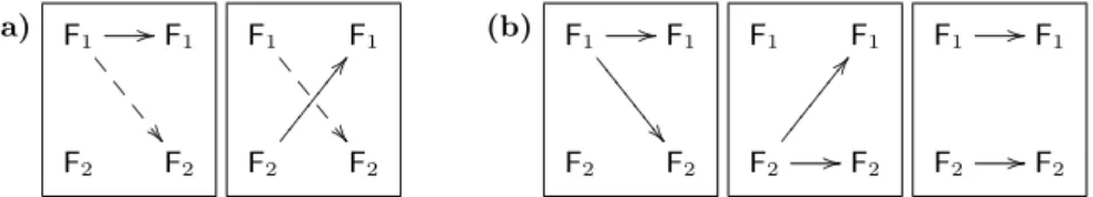
Fig. 1.Size-change graphs from Ex. 2

undecidable termination problem is abstracted to a decidable one. For SCT, we use a base order to obtain the finite representation of the paths by size-change graphs. For DPs, no such abstraction is performed and, indeed, the termination of a DP problem is undecidable. Here, the abstraction step is only the second stage where typically a decidable class of base orders is used.

The SCT method can be used with any base order. It only requires the infor- mation which arguments of a function call become (strictly or weakly) smaller w.r.t. the base order. To prove termination, the base order has to be well founded.

For the adaptation to TRSs we will use a reduction pair (%,) for this purpose and introduce the notion of a size-change graph directly for dependency pairs.

If the TRS has a DPF(s1, . . . , sn)→G(t1, . . . , tm), then the corresponding size-change graph has nodes{F1, . . . , Fn, G1, . . . , Gm}representing the argument positions ofFandG. The labeled edges in the size-change graph indicate whether there is a strict or weak decrease between these arguments.

Definition 1 (size-change graphs).Let(%,)be a (possibly non-monotonic) reduction pair on base terms, and letF(s1, . . . , sn)→G(t1, . . . , tm)be a DP. The size-change graph resulting from this DP and this reduction pair is the graph (Vs, Vt, E)with source vertices Vs={F1, . . . , Fn}, target verticesVt={G1, . . . , Gm}, and labeled edgesE={(Fi, Gj,)|sitj} ∪ {(Fi, Gj,%)|si%tj}.

Size-change graphs are depicted as in Fig. 1. Each graph consists of source vertices, on the left, target vertices, on the right, and edges drawn as full and dashed arrows to indicate strict and weak decrease (i.e., corresponding to “”

and “%”, respectively). We introduce the main ideas underlying SCT by example.

Example 2. Consider the TRS {(1),(2)}. It has the DPs (3) and (4).

f(s(x), y)→f(x,s(x)) (1) f(x,s(y))→f(y, x) (2)

F(s(x), y)→F(x,s(x)) (3) F(x,s(y))→F(y, x) (4) We use a reduction pair based on the embedding order wheres(x)x,s(y)y, s(x)%s(x), s(y) %s(y). Then we get the size-change graphs in Fig. 1(a). Be- tween consecutive function calls, the first argument decreases in size or becomes smaller than the original second argument. In both cases, the second argument weakly decreases compared to the original first argument. By repeated composition of the size-change graphs, we obtain the three “idempotent” graphs in Fig. 1(b). All of them exhibitin situ decrease (atF₁ in the first graph, atF₂in the second graph, and at both F1 and F2 in the third graph). This means that the original size-change graphs from Fig. 1(a)satisfy the SCT property.

(5)

Earlier work [29] shows how to combine SCT with term rewriting. LetRbe a TRS and (%,) a reduction pair such that ifst(or s%t) thentcontains no defined symbols of R, i.e., no root symbols of left-hand sides of rules from R.⁵LetGbe the set of size-change graphs resulting from all DPs with (%,). In [29] the authors prove that if Gsatisfies SCT thenRis innermost terminating.

Example 3. If one restricts the reduction pair in Ex. 2 to just terms without defined symbols, then one still obtains the same size-change graphs. Since these graphs satisfy the SCT property, one can conclude that the TRS is indeed innermost terminating. Note that to show termination without SCT, an order like RPO would fail (since the first rule requires a lexicographic comparison and the second requires a multiset comparison). While termination could be proved by polynomial orders, as in [29] one could unite these rules with the rules for the Ackermann function. Then SCT with the embedding order would still work, whereas a direct application of RPO or polynomial orders fails.

So our example illustrates a major strength of SCT. A proof of termination is obtained by using just a simple base order and by considering each idempotent graph in the closure under composition afterwards. In contrast, without SCT, one would need more complex termination arguments.

In [29] the authors show that when constructing the size-change graphs from the DPs, one can even use arbitrary reduction pairs as base orders, provided that all rules of the TRS are weakly decreasing. In other words, this previous work essentially addresses the following question for any DP problem (P,R):

For a given base order whereRis weakly decreasing, do all idempotent size-change graphs, under composition closure, exhibit in situ decrease?

Note that in [29], the base order is always given and the only way to search for a base order automatically would be a hopeless generate-and-test approach.

4 Approximating SCT in NP

In [5] the authors identify a subset of SCT, called SCNP, that is powerful enough for practical use and is in NP. For SCNP just as for SCT, programs are abstracted to sets of size-change graphs. But instead of checking SCT by the closure under composition, one identifies a suitable ranking function to certify the termination of programs described by the set of graphs. Ranking functions map “program states” to elements of a well-founded domain and one has to show that they (strictly) decrease on all program transitions described by the size-change graphs.

In the rewriting context, program states are terms. Here, instead of a ranking function one can use an arbitrary stable well-founded orderA. Let (V_s, V_t, E) be a size-change graph with source verticesVs={F1, . . . , Fn}, target verticesVt= {G1, . . . , Gm}, and let (%,) be the reduction pair on base terms which was used for the construction of the graph. Now the goal is to extend the orderto a well-founded orderAwhich can also compare tuple terms and whichsatisfies

5 Strictly speaking, this is not a reduction pair, since it is only stable under substitu- tions which do not introduce defined symbols.

(6)

the size-change graph (i.e.,F(s₁, . . . , s_n)AG(t₁, . . . , t_m)). Similarly, we say that Asatisfies aset of size-change graphs iff it satisfies all the graphs in the set.

If the size-change graphs describe the transitions of a program, then the existence of a corresponding ranking function obviously implies termination of the program. As in [29], to ensure that the size-change graphs really describe the transitions of the TRS correctly, one has to impose suitable restrictions on the reduction pair (e.g., by demanding that all rules of the TRS are weakly decreasing w.r.t.%). Then one can indeed conclude termination of the TRS.

In [22], a class of ranking functions is identified which can simulate SCT.

So if a set of size-change graphs has the SCT property, then there is a ranking function of that class satisfying these size-change graphs. However, this class is typically exponential in size [22]. To obtain a subset of SCT in NP, [5] considers a restricted class of ranking functions. A set of size-change graphs has theSCNP property iff it is satisfied by a ranking function from this restricted class.

Our goal is to adapt this class of ranking functions to term rewriting. The main motivation is to facilitate thesimultaneous search for a ranking function on the size-change graphs and for the base order which is used to derive the size- change graphs from a TRS. It means that we are searching both for a program abstraction to size-change graphs, and also for the ranking function which proves that these graphs have the SCNP (and hence also the SCT) property.

This is different from [5], where the concrete structure of the program has already been abstracted away to size-change graphs that must be given as inputs. It is also different from the earlier adaption of SCT to term rewriting in [29], where the base order was fixed. As shown by the experiments with [29] in Sect. 6, fixing the base order for the size-change graphs leads to severe limitations in power.

The following example illustrates the SCNP property and presents a ranking function (resp. a well-founded orderA) satisfying a set of size-change graphs.

Example 4. Consider the TRS from Ex. 2 and its size-change graphs in Fig. 1(a).

Here, the base order is the reduction pair (%,) resulting from the embedding order. We now extendto an orderAwhich can also compare tuple terms and which satisfies the size-change graphs in this example. To compare tuple terms F(s1, s2) andF(t1, t2), we first map them to the multisets { hs1,1i,hs2,0i }and { ht1,1i,ht2,0i }of tagged terms (where a tagged term is a pair of a term and a number). Now a multisetS of tagged terms is greater than a multiset T iff for every ht, mi ∈T there is anhs, ni ∈S wherest or boths%tandn > m.

For the first graph, we have s₁ t₁ and s₁ % t₂ and hence the multiset { hs₁,1i,hs₂,0i }is greater than{ ht₁,1i,ht₂,0i }. For the second graph,s₁ %t₂ and s₂ t₁ also implies that the multiset { hs₁,1i, hs₂,0i } is greater than { ht1,1i,ht2,0i }. Thus, if we define our well-founded order Ain this way, then it indeed satisfies both size-change graphs of the example. Since this order A belongs to the class of ranking functions defined in [5], this shows that the size- change graphs in Fig. 1(a)have the SCNP property.

In term rewriting, size-change graphs correspond to DPs and the arcs of the size-change graphs are built by only comparing the arguments of the DPs (which arebase terms). The ranking function then corresponds to a well-founded order

(7)

on tuple terms. We now reformulate the class of ranking functions of [5] in the term rewriting context by definingSCNP reduction pairs. The advantage of this reformulation is that it allows us to integrate the SCNP approach directly into the DP framework and that it allows a SAT encoding of both the search for suitable base orders and of the test for the SCNP property. In [5], the class of ranking functions for SCNP is defined incrementally. We follow this, but adapt the definitions of [5] to the term rewriting setting and prove that the resulting orders always constitute reduction pairs. More precisely, we proceed as follows:

step one: (%,) is an arbitrary reduction pair on base terms that we start with (e.g., based on RPO and argument filters or on polynomial orders). The main observation that can be drawn from the SCNP approach is that it is helpful to compare base terms and tuple terms in a different way. Thus, our goal is to extend (%,) appropriately to a reduction pair (w,A) that can also compare tuple terms. By defining (w,A) in the same way as the ranking functions of [5], it can simulate the SCNP approach.

step two: (%^N,^N) is a reduction pair on tagged base terms, i.e., on pairs ht, ni, wheretis a base term andn∈N. Essentially, (%^N,^N) is a lexicographic combination of the reduction pair (%,) with the usual order onN.

step three: (%^N^,µ,^N^,µ) extends (%^N,^N) to comparemultisetsof tagged base terms. Thestatus µdetermines how (%^N,^N) is extended to multisets.

step four: (%^µ,`,^µ,`) is a full reduction pair (i.e., it is the reduction pair (w,A) we were looking for). Thelevel mapping ` determines which arguments of a tuple term are selected and tagged, resulting in a multiset of tagged base terms. On tuple terms, (%^µ,`,^µ,`) behaves according to (%^N^,µ,^N^,µ) on the multisets as determined by`, and on base terms, it behaves like (%,).

Thus, we start with extending a reduction pair (%,) on base terms to a reduction pair (%^N,^N) on tagged base terms. We compare tagged terms lexi- cographically by (%,) and by the standard orders≥and>on numbers.

Definition 5 (comparing tagged terms). Let (%,) be a reduction pair on terms. We define the corresponding reduction pair(%^N,^N)on tagged terms:

– ht₁, n₁i%^Nht₂, n₂i ⇔ t₁t₂ ∨ (t₁%t₂∧n₁≥n₂).

– ht1, n1i ^Nht2, n2i ⇔ t1t2 ∨ (t1%t2∧n1> n2).

The motivation for tagged terms is that we will use different tags (i.e., numbers) for the different argument positions of a function symbol. For instance, when comparing the terms s = F(s(x), y) and t = F(x,s(x)) as in Ex. 4, one can assign the tags 1 and 0 to the first and second argument position ofF, respectively. Then, if (%,) is the reduction pair based on the embedding order, we have hs(x),1i ^N hx,1i and hs(x),1i ^N hs(x),0i. In other words, the first argument ofsis greater than both the first and the second argument oft.

The following lemma states that if (%,) is a reduction pair on terms, then (%^N,^N) is a reduction pair on tagged terms (where we do not require monotonicity, since monotonicity is not defined for tagged terms). This lemma will be needed for our main theorem (Thm. 12) which proves that the reduction pair defined to simulate SCNP is really a reduction pair.

(8)

Lemma 6 (reduction pairs on tagged terms). Let (%,) be a reduction pair. Then(%^N,^N)is a non-monotonic reduction pair on tagged terms.⁶

The next step is to introduce a “reduction pair” (%^N^,µ,^N^,µ) on multisets of tagged base terms, whereµis a status which determines how (%^N,^N) is extended to multisets. Of course, there are many possibilities for such an extension.

In Def. 7, we present the four extensions which correspond to the ranking functions defining SCNP in [5]. The main difference to the definitions in [5] is that we do not restrict ourselves tototal base orders. Hence, the notions of maximum and minimum of a multiset of terms are not defined in the same way as in [5].

Definition 7 (multiset extensions of reduction pairs). Let (%,) be a reduction pair on (tagged) terms. We define an extended reduction pair(%^µ,^µ) on multisets of (tagged) terms, for µ ∈ {max, min, ms, dms}. Let S and T be multisets of (tagged) terms.

1. (max order)S %^maxT holds iff∀t∈T.∃s∈S. s%t.

S^maxT holds iff S6=∅and∀t∈T.∃s∈S. st.

2. (min order)S%^minT holds iff∀s∈S.∃t∈T. s%t.

S^minT holds iffT 6=∅and∀s∈S.∃t∈T. st.

3. (multiset order [10]) S ^ms T holds iff S = Sstrict ]

s1, . . . , sk , T = T_strict]

t₁, . . . , t_k ,S_strict^maxT_strict, ands_i %t_i for1≤i≤k.

S %^ms T holds iff S = Sstrict ]

s1, . . . , sk , T = Tstrict]

t1, . . . , tk , eitherSstrict ^maxTstrict or Sstrict=Tstrict=∅, andsi%ti for1≤i≤k.

4. (dual multiset order [4]) S ^dms T holds iff S = Sstrict ]

s1, . . . , sk , T =T_strict]

t1, . . . , tk ,S_strict^minT_strict, ands_i%t_i for1≤i≤k.

S %^dms T holds iff S =Sstrict]

s₁, . . . , s_k , T = Tstrict]

t₁, . . . , t_k , eitherSstrict ^minTstrict orSstrict=Tstrict=∅, andsi%ti for1≤i≤k.

Here^ms is to the standard multiset extension of an order as used, e.g., for the classical definition of RPO. However, our use of tagged terms as elements of the multiset introduces a lexicographic aspect that is missing in RPO.

Example 8. Consider again the TRS from Ex. 2 with the reduction pair based on the embedding order. We have{s(x), y}%^max{x,s(x)}, since for both terms in {x,s(x)} there is an element in {s(x), y} which is weakly greater (w.r.t.%).

Similarly, {x,s(y)} %^max {y, x}. However, {x,s(y)} 6^max {y, x}, since not every element from {y, x} has a strictly greater one in {x,s(y)}. We also have {x,s(y)}%^min{y, x}, but{s(x), y} 6%^min{x,s(x)}, since foryin{s(x), y}, there is no term in{x,s(x)}which is weakly smaller.

We have{s(x), y} 6^ms {x,s(x)}, since even if we take {s(x)} ^max{x}, we still do not have y % s(x). Moreover, also {s(x), y} 6%^ms {x,s(x)}. Otherwise, for every element of{x,s(x)} there would have to be adifferent weakly greater element in{s(x), y}. In contrast, we have{x,s(y)} ^ms{y, x}. The elements(y) is replaced by the strictly smaller elementy and for the remaining elementxon the right-hand side there is a weakly greater one on the left-hand side. Similarly, we also have {s(x), y} 6%^dms{x,s(x)}and{x,s(y)} ^dms {y, x}.

6 All proofs can be found in [6].

(9)

So there is no µ such that the multiset of arguments strictly decreases in some DP and weakly decreases in the other DP. We can only achieve a weak decrease for all DPs. To obtain a strict decrease in such cases, one can add tags.

We want to define a reduction pair (%^µ,`,^µ,`) which is like (%^N^,µ,^N^,µ) on tuple terms and like (%,) on base terms. Here, we use a level mapping ` to map tuple termsF(s1, . . . , sn) to multisets of tagged base terms.

Definition 9 (level mapping).For each tuple symbolF of arityn, letπ(F)⊆ 1, . . . , n ×N such that for each 1 ≤j ≤n there is at most one m∈N with hj, mi ∈π(F). Then`(F(s₁, . . . , s_n)) =

hs_i, n_ii

hi, n_ii ∈π(F) .

Example 10. Consider again the TRS from Ex. 2 with the reduction pair based on the embedding order. Letπbe a status function withπ(F) =

h1,1i,h2,0i . Soπselects both arguments of terms rooted withFfor comparison and associates the tag 1 with the first argument and the tag 0 with the second argument. This means that it puts “more weight” on the first than on the second argument. The level mapping ` defined by π transforms the tuple terms from the DPs of our TRS into the following multisets of tagged terms:

`(F(s(x), y)) =

hs(x),1i,hy,0i `(F(x,s(x))) =

hx,1i,hs(x),0i

`(F(x,s(y))) =

hx,1i,hs(y),0i `(F(y, x)) =

hy,1i,hx,0i Now we observe that for the multisets of the tagged terms above, we have

`(F(s(x), y)) ^N^,max `(F(x,s(x))) `(F(x,s(y))) ^N^,max `(F(y, x)) So due to the tagging now we can find an order such that both DPs are strictly decreasing. This order corresponds to the ranking function given in Ex. 4.

Finally we define the class of reduction pairs which corresponds to the class of ranking functions considered for SCNP in [5].

Definition 11 (SCNP reduction pair). Let (%,) be a reduction pair on base terms and let`be a level mapping. Forµ∈ {max, min, ms, dms}, we define the SCNP reduction pair (%^µ,`,^µ,`). For base termsl, rwe definel ₍%)

µ,`r ⇔ l ₍%)r and for tuple termssand twe define

So we haves ^max,` tfor the DPss→tin Ex. 2 and the level mapping`in Ex. 10. Thm. 12 states that SCNP reduction pairs actuallyare reduction pairs.

Theorem 12. Forµ∈ {max, min, ms, dms},(%^µ,`,^µ,`)is a reduction pair.

We now automate the SCNP criterion of [5]. For a DP problem (P,R) with the DPsP and the TRSR, we have to find a suitable base order (%,) to con- struct the size-change graphsG corresponding to the DPs inP. So every graph (V_s, V_t, E) fromGwith source verticesV_s={F1, . . . , F_n}and target verticesV_t= {G1, . . . , G_m}corresponds to a DPF(s₁, . . . , s_n)→G(t₁, . . . , t_m). Moreover, we have an edge (F_i, G_j,)∈E iffs_it_j and (F_i, G_j,%)∈Eiffs_i%t_j.

In our example, if we use the reduction pair (%,) based on the embedding order, thenG are the size-change graphs from Fig. 1(a). For instance, the first size-change graph results from the DP (3).

For SCNP, we have to extend to a well-founded orderA which can also

(10)

compare tuple terms and which satisfies all size-change graphs in G. For A, we could take any order ^µ,` from an SCNP reduction pair (%^µ,`,^µ,`). To show that A satisfies the size-change graphs from G, one then has to prove F(s1, . . . , sn) ^µ,` G(t1, . . . , tm) for every DP F(s1, . . . , sn) → G(t1, . . . , tm).

Moreover, to ensure that the size-change graphs correctly describe the transitions of the TRS-programR, one also has to require that all rules of the TRSRare weakly decreasing w.r.t. % (cf. the remarks at the beginning of Sect. 4). Of course, as in [29], this requirement can be weakened (e.g., by only regarding usable rules) when provinginnermost termination.

As in [5], we as a lexicographic combination of several orders of the form ^µ,`. We define the lexicographic combination of two reduction pairs as (%¹,1

)×(%²,2) = (%1×2,_1×2). Here, s %1×2 t holds iff both s%¹ t and s %² t.

Moreover, s_1×2 t holds iff s1 t or both s%¹ t and s2 t. It is clear that (%1×2,_1×2) is again a reduction pair.

A suitable well-founded orderAis now constructed automatically as follows.

The pair of orders (w,A) is initialized by defining w to be the relation where onlytwtholds for two tuple or base termstand whereAis the empty relation.

As long as the set of size-change graphs G is not empty, a statusµand a level mapping ` are synthesized such that (%^µ,`,^µ,`) orients all DPs weakly and at least one DP strictly. In other words, the corresponding ranking function satisfies one size-change graph and “weakly satisfies” the others. Then the strictly oriented DPs (resp. the strictly satisfied size-change graphs) are removed, and (w,A) := (w,A)×(%^µ,`,^µ,`) is updated. In this way, the SCNP approach can be simulated by a repeated application of thereduction pair processor in the DP framework, using the special class of SCNP reduction pairs.

So in our example, we could first look for aµ1and`1 where the first DP (3) decreases strictly (w.r.t.^µ¹^,`¹) and the second decreases weakly (w.r.t.%^µ¹^,`¹).

Then we would remove the first DP and could now search for aµ2 and`2 such that the remaining second DP (4) decreases strictly (w.r.t.^µ²^,`²). The resulting reduction pair would be (w,A) = (%^µ¹^,`¹,^µ¹^,`¹)×(%^µ²^,`²,^µ²^,`²).

While in [5], the set of size-change graphs remains fixed throughout the whole termination proof, the DP framework allows to use a lexicographic combination of SCNP reduction pairs which are constructed from different reduction pairs (%,) on base terms. In other words, after a base order and a ranking function satisfying one size-change graph and weakly satisfying all others have been found, the satisfied size-change graph (resp. the corresponding DP) is removed, and one can synthesize a possibly different ranking function and also apossibly different base order for the remaining DPs (i.e., different abstractions to different size- change graphs can be used in one single termination proof).

Example 13. We add a third rule to the TRS from Ex. 2:f(c(x), y)→f(x,s(x)).

Now no SCNP reduction pair based only on the embedding order can orient all DPs strictly at the same time anymore, even if one permits combinations with arbitrary argument filters. However, we can first apply an SCNP reduction pair that sets all tags to 0 and uses the embedding order together with an argument filter to collapse the symbolsto its argument. Then the DP for the newly added

(11)

rule is oriented strictly and all other DPs are oriented weakly. After removing the new DP, the SCNP reduction pair that we already used for the DPs of Ex. 2 again orients all DPs strictly. Note that the base order for this second SCNP reduction pair is the embedding order without argument filters, i.e., it differs from the base order used in the first SCNP reduction pair.

By representing the SCNP method via SCNP reduction pairs, we can now benefit from the flexibility of the DP framework. Thus, we can use other termination methods in addition to SCNP. More precisely, as usual in the DP framework, we can apply arbitrary processors one after another in a modular way. This allows us to interleave arbitrary other termination techniques with termination proof steps based on size-change termination, whereas in [29], size-change proofs could only be used as a final step in a termination proof.

5 Automation by SAT Encoding

Recently, the search problem for many common base orders has been reduced successfully to SAT problems [8, 9, 13, 26, 30]. In this section, we build on this earlier work and use these encodings as components for a SAT encoding of SCNP reduction pairs. The corresponding decision problem is stated as follows:

For a DP problem (P,R) and a given class of base orders, is there a status µ, a level mapping`, and a concrete base reduction pair (%,) such that the SCNP reduction pair (%^µ,`,^µ,`) orients all rules ofRand P weakly and at least one ofP strictly?

We assume a given base SAT encoding J.K^base which maps base term constraints of the forms₍%)tto propositional formulas. Every satisfying assignment for the formulaJs₍%)tK^basecorresponds to a particular order wheres₍%)tholds.

We also assume a given encoding for partial orders (on tags), cf. [9]. The function J.Kpo maps partial order constraints of the form n1 ≥ n2 or n1 > n2

where n₁ and n₂ represent natural numbers (in some fixed number of bits) to corresponding propositional formulas on the bit representations for the numbers.

For brevity, we only show the encoding for SCNP reduction pairs (%^µ,`,^µ,`) whereµ=max. The encodings for the other cases are similar: The encoding for the min comparison is completely analogous. To encode (dual) multiset comparison one can adapt previous approaches to encode multiset orders [26].

First, for each tuple symbolF of arityn, we introduce natural number variables denoted tag^F_i for 1 ≤i ≤ n. These encode the tags associated with the argument positions ofF by representing them in a fixed number of bits. In our case, it suffices to consider tag values which are less than the sum of the arities of the tuple symbols. In this way, every argument position of every tuple symbol could get a different tag, i.e., this suffices to represent all possible level mappings.

Now consider a size-change graph corresponding to a DP δ = s → t with s=F(s1, . . . , sn) andt=G(t1, . . . , tm). The edges of the size-change graph are determined by the base order, which is not fixed. For any 1 ≤i ≤n and 1 ≤ j ≤m, we define a propositional formulaweak^δ_i,j which is true iffhs,tag^F_i i%^N ht,tag^G_ji. Similarly,strict^δ_i,j is true iff hs,tag^F_i i ^N ht,tag^G_ji. The definition of

(12)

weak^δ_i,j andstrict^δ_i,j corresponds directly to Def. 5. It is based on the encodings J.Kbase andJ.Kpo for the base order and for the tags, respectively.

weak^δ_i,j=JsitjK^base ∨ (Jsi%tjK^base∧Jtag^F_i ≥tag^G_j K^po) strict^δ_i,j=JsitjK^base ∨ (Jsi%tjK^base∧Jtag^F_i >tag^G_j K^po)

To facilitate the search for level mappings, for each tuple symbol F of arity n we introduce propositional variables reg^F_i for 1 ≤ i ≤ n. Here, reg^F_i is true iff the i-th argument position of F is regarded for comparison. The formulas Js%^max,`tK and Js^max,`tK then encode that the DP s → t can be oriented weakly or strictly, respectively. By this encoding, one can simultaneously search for a base order that gives rise to the edges in the size-change graph and for a level mapping that satisfies this size-change graph.

Js%^max,`tK= ^

1≤j≤m

(reg^G_j → _

1≤i≤n

(reg^F_i ∧weak^δ_i,j))

Js^max,`tK= ^

1≤j≤m

(reg^G_j → _

1≤i≤n

(reg^F_i ∧strict^δ_i,j)) ∧ _

1≤i≤n

reg^F_i

For any DP problem (P,R) we can now generate a propositional formula which ensures that the corresponding SCNP reduction pair orients all rules from R andP weakly and at least one rule fromP strictly:

^

l→r∈R

Jl%rK^base ∧ ^

s→t∈P

Js%^max,`tK ∧ _

s→t∈P

Js^max,`tK Similar to [8, 30], our approach is easily extended to refinements of the DP method where one only regards the usable rules of R and where these usable rules can also depend on the (explicit or implicit) argument filter of the order.

6 Implementation and Experiments

We implemented our contributions in the automated termination proverAProVE [15]. To assess their impact, we compared three configurations of AProVE. In the first, we use SCNP reduction pairs in the reduction pair processor of the DP framework. This configuration is parameterized by the choice whether we allow just max comparisons of multisets or all four multiset extensions from Def. 7.

Moreover, the configuration is also parameterized by the choice whether we use classical size-change graphs or extended size-change graphs as in [29]. In an extended size-change graph, to compares=F(s1, . . . , sn) witht=G(t1, . . . , tm), the source and target vertices{s1, . . . , s_n}and{t1, . . . , t_m}are extended by additional verticess and t, respectively. Now an edge from sto t_j indicates that the whole term s is greater (or equal) to t_j, etc. So these additional vertices also allow us to compare the whole terms s and t. By adding these vertices, size-change termination incorporates the standard comparison of terms as well.

In the second configuration, we use the base orders directly in the reduction pair processor (i.e., here we disregard SCNP reduction pairs). In the third configuration, we use the implementation of the SCT method as described in [29]. For

(13)

order SCNP fast SCNP max SCNP all reduction pairs SCT [29]

EMB proved 346 346 347 325 341

runtime 2882.6 3306.4 3628.5 2891.3 10065.4

LPO proved 500 530 527 505 385

runtime 3093.7 5985.5 7739.2 3698.4 10015.5

RPO proved 501 531 531 527 385

runtime 3222.2 6384.1 8118.0 4027.5 10053.4

POLO proved 477 514 514 511 378

runtime 3153.6 5273.6 7124.4 2941.7 9974.0

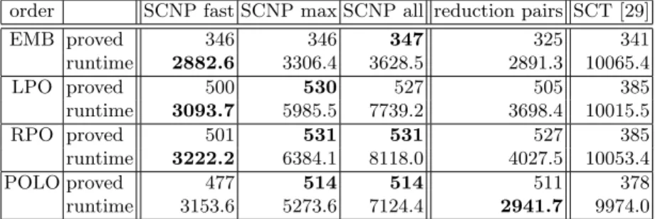
Table 1.Comparison of SCNP reduction pairs to SCT and direct reduction pairs.

a fair comparison, we updated that old implementation from the DPapproach to the modular DPframeworkand used SAT encodings for the base orders. (While this approach only uses the embedding order and argument filters as the base order for the construction of size-change graphs, it uses more complex orders (containing the base order) to weakly orient the rules from the TRS.)

We considered all 1381 examples from the standard TRS category of theTer- mination Problem Data Base (TPDB version 7.0.2) as used in theInternational Termination Competition2009.⁷ The experiments were run on a 2.66 GHz Intel Core 2 Quad and we used a time limit of 60 seconds per example. We applied SAT4J[20] to transform propositional formulas to conjunctive normal form and the SAT solverMiniSAT2[11] to check the satisfiability of the resulting formulas.

Table 1 compares the power and runtimes of the three configurations depend- ing on the base order. The column “order” indicates the base order: embedding order with argument filters (EMB), lexicographic path order with arbitrary per- mutations and argument filters (LPO), recursive path order with argument filters (RPO), and linear polynomial interpretations with coefficients from{0,1}

(POLO). For the first configuration, we used three different settings: full SCNP reduction pairs with extended size-change graphs (“SCNP all”), SCNP reduction pairs restricted to max-comparisons with extended size-change graphs (“SCNP max”), and SCNP reduction pairs restricted to max comparisons and non- extended size-change graphs (“SCNP fast”). The second and third configuration are called “reduction pairs” and “SCT [29]”, respectively. For each experiment, we give the number of TRSs which could be proved terminating (“proved”) and the analysis time in seconds for runningAProVEon all 1381 TRSs (“runtime”).

The “best” numbers are always printed inbold. For further details on the experiments, we refer to http://aprove.informatik.rwth-aachen.de/eval/SCNP.

The table allows the following observations:

(1)Our SCNP reduction pairs are much more powerful and significantly faster than the implementation of [29]. By integrating the search for the base order with SCNP, our new implementation can use a much larger class of base orders and thus, SCNP reduction pairs can prove significantly more examples. The reason for the relatively low speed of [29] is that this approach iterates through argument filters and then generates and analyzes size-change graphs for each of

7 http://www.termination-portal.org/wiki/Termination_Competition/

(14)

these argument filters. (So the low speed is not due to the repeated composition of size-change graphs in the SCT criterion.)

(2) Our new implementation of SCNP reduction pairs is more powerful than using the reduction pairs directly. Note that when using extended size-change graphs, every reduction pair can be simulated by an SCNP reduction pair.

(3)SCNP reduction pairsadd significant power when used for simple orderslike EMB and LPO. The difference is less dramatic for RPO and POLO. Intuitively, the reason is that SCNP allows for multiset comparisons which are lacking in EMB and LPO, while RPO contains multiset comparisons and POLO can often simulate them. Nevertheless, SCNP also adds some power to RPO and POLO, e.g., by extending them by a concept like “maximum”. This even holds for more powerful base orders like matrix orders [12]. In [6], we present a TRS where all existing termination tools fail, but where termination can easily be proved automatically by an SCNP reduction pair with a matrix base order.

7 Conclusion

We show that the practically relevant part of size-change termination (SCNP) can be formulated as a reduction pair. Thus, SCNP can be applied in the DP framework, which is used in virtually all termination tools for term rewriting.

Moreover, by combining the search for the base order and for the SCNP level mapping into one search problem, we can automatically find the right base order for constructing size-change graphs. Thus, we now generate program abstractions automatically such that termination of the abstracted program can be shown.

The implementation inAProVEconfirms the usefulness of our contribution.

Our experiments indicate that the automation of our technique is more powerful than both the direct use of reduction pairs and the SCT adaptation from [29].

References

1. T. Arts and J. Giesl. Termination of term rewriting using dependency pairs. The- oretical Computer Science, 236:133–178, 2000.

2. J. Avery. Size-change termination and bound analysis. InProc. FLOPS ’06, LNCS 3945, pages 192–207, 2006.

3. F. Baader and T. Nipkow. Term Rewriting and All That. Cambridge, 1998.

4. A. M. Ben-Amram and C. S. Lee. Size-change termination in polynomial time.

ACM Transactions on Programming Languages and Systems, 29(1), 2007.

5. A. M. Ben-Amram and M. Codish. A SAT-based approach to size change termination with global ranking functions. In Proc. TACAS ’08, LNCS 4963, pages 218–232, 2008.

6. M. Codish, C. Fuhs, J. Giesl, and P. Schneider-Kamp. Lazy abstraction for size- change termination. Technical Report AIB-2010-14, RWTH Aachen University, 2010. http://aib.informatik.rwth-aachen.de.

7. M. Codish and C. Taboch. A semantic basis for termination analysis of logic programs. Journal of Logic Programming, 41(1):103–123, 1999.

8. M. Codish, P. Schneider-Kamp, V. Lagoon, R. Thiemann, and J. Giesl. SAT solving for argument filterings. InProc. LPAR ’06, LNAI 4246, pages 30–44, 2006.

9. M. Codish, V. Lagoon, and P. Stuckey. Solving partial order constraints for LPO

(15)

termination.J. Satisfiability, Boolean Modeling and Computation, 5:193–215, 2008.

10. N. Dershowitz and Z. Manna. Proving termination with multiset orderings. Com- munications of the ACM, 22(8):465–476, 1979.

11. N. E´en and N. S¨orensson. MiniSAT. http://minisat.se.

12. J. Endrullis, J. Waldmann, and H. Zantema. Matrix interpretations for proving termination of term rewriting. J. Automated Reasoning, 40(2-3):195–220, 2008.

13. C. Fuhs, J. Giesl, A. Middeldorp, R. Thiemann, P. Schneider-Kamp, and H. Zankl.

SAT solving for termination analysis with polynomial interpretations. In Proc.

SAT ’07, LNCS 4501, pages 340–354, 2007.

14. J. Giesl, R. Thiemann, and P. Schneider-Kamp. The dependency pair framework:

Combining techniques for automated termination proofs. InProc. LPAR ’04, LNAI 3542, pages 301–331, 2005.

15. J. Giesl, P. Schneider-Kamp, and R. Thiemann. AProVE 1.2: Automatic termination proofs in the dependency pair framework. InProc. IJCAR ’06, LNAI 4130, pages 281–286, 2006.

16. J. Giesl, R. Thiemann, P. Schneider-Kamp, and S. Falke. Mechanizing and im- proving dependency pairs. Journal of Automated Reasoning, 37(3):155–203, 2006.

17. J. Giesl, M. Raffelsieper, P. Schneider-Kamp, S. Swiderski, and R. Thiemann.

Automated termination proofs forHaskellby term rewriting. ACM Transactions on Programming Languages and Systems, 2010. To appear. Preliminary version appeared inProc. RTA ’06, LNCS, 4098, pages 297-312, 2006.

18. N. Hirokawa and A. Middeldorp. Automating the dependency pair method. In- formation and Computation, 199(1,2):172–199, 2005.

19. N. D. Jones and N. Bohr. Termination analysis of the untyped lambda calculus.

InProc. RTA ’04, LNCS 3091, pages 1–23, 2004.

20. D. Le Berre and A. Parrain. SAT4J. http://www.sat4j.org.

21. C. S. Lee, N. D. Jones, and A. M. Ben-Amram. The size-change principle for program termination. InProc. POPL ’01, pages 81–92, 2001.

22. C. S. Lee. Ranking functions for size-change termination. ACM Transactions on Programming Languages and Systems, 31(3):1–42, 2009.

23. M. T. Nguyen, D. De Schreye, J. Giesl, and P. Schneider-Kamp. Polytool: Polyno- mial interpretations as a basis for termination analysis of logic programs. Theory and Practice of Logic Programming, 2010. To appear.

24. C. Otto, M. Brockschmidt, C. von Essen, and J. Giesl. Automated termination analysis of Java Bytecodeby term rewriting. In Proc. RTA ’10, LIPIcs 6, pages 259–276, 2010.

25. A. Podelski and A. Rybalchenko. Transition Invariants. InProc. 19th LICS, pages 32–41. IEEE, 2004.

26. P. Schneider-Kamp, R. Thiemann, E. Annov, M. Codish, and J. Giesl. Proving termination using recursive path orders and SAT solving. In Proc. FroCoS ’07, LNAI 4720, pages 267–282, 2007.

27. P. Schneider-Kamp, J. Giesl, A. Serebrenik, and R. Thiemann. Automated termination proofs for logic programs by term rewriting. ACM Transactions on Com- putational Logic, 11(1):1–52, 2009.

28. D. Sereni and N. D. Jones. Termination analysis of higher-order functional programs. InProc. APLAS ’05, LNCS 3780, pages 281–297, 2005.

29. R. Thiemann and J. Giesl. The size-change principle and dependency pairs for termination of term rewriting. Applicable Algebra in Engineering, Communication and Computing, 16(4):229–270, 2005.

30. H. Zankl, N. Hirokawa, and A. Middeldorp. KBO orientability. Journal of Auto- mated Reasoning, 43(2):173–201, 2009.