Automated Termination Proofs for Java Programs with Cyclic Data
?Marc Brockschmidt, Richard Musiol, Carsten Otto, and J¨urgen Giesl
LuFG Informatik 2, RWTH Aachen University, Germany
Abstract. In earlier work, we developed a technique to prove termina- tion of Javaprograms automatically: first,Javaprograms are automat- ically transformed to term rewrite systems (TRSs) and then, existing methods and tools are used to prove termination of the resulting TRSs.
In this paper, we extend our technique in order to prove termination of algorithms on cyclic data such as cyclic lists or graphs automatically. We implemented our technique in the toolAProVEand performed extensive experiments to evaluate its practical applicability.
1 Introduction
Techniques to prove termination automatically are essential in program verifi- cation. While approaches and tools for automated termination analysis of term rewrite systems (TRSs) and oflogic programs have been studied for decades, in the last years the focus has shifted toward imperative languages like CorJava.
Most techniques for imperative languages prove termination by synthesizing ranking functions (e.g., [12, 26]) and localize the termination test using Ramsey’s theorem [23, 27]. Such techniques are for instance used in the toolsTerminator[4, 13] andLoopFrog [22, 31] to analyze termination of Cprograms. To handle the heap, one can use an abstraction [14] to integers based on separation logic [24].
On the other hand, there also existtransformational approaches which au- tomatically transform imperative programs to TRSs or to logic programs. They allow to re-use the existing techniques and tools from term rewriting or logic programming also for imperative programs. In [17],Cis analyzed by a transfor- mation to TRSs and the toolsJulia[30] andCOSTA[2] prove termination of Java via a transformation to constraint logic programs. To deal with the heap, they also use an abstraction to integers and represent objects by theirpath length.
In [6–8, 25] we presented an alternative approach for termination ofJavavia a transformation to TRSs. Like [2, 30], we considerJava Bytecode(JBC) to avoid dealing with all language constructs of Java. This is no restriction, since Java compilers automatically translateJavatoJBC. Indeed, our implementation han- dles theJava Bytecode produced by Oracle’s standard compiler. In contrast to other approaches, we do not treat the heap by an abstraction to integers, but by an abstraction toterms. So for any classClwith nnon-static fields, we use ann-ary function symbolCl. For example, consider a classList with two fields value andnext. Then every List object is encoded as a term List(v, n) where
?Supported by the DFG grant GI 274/5-3
v is the value of the current element andnis the encoding of the next element.
Hence, a list “[1,2]” is encoded by the termList(1,List(2,null)). In this way, our encoding maintains much more information from the original program than a (fixed) abstraction to integers. Now the advantage is that for any algorithm, ex- isting tools from term rewriting can automatically search for (possibly different) suitable well-founded orders comparing arbitrary forms of terms. For more in- formation on techniques for termination analysis of term rewriting, see, e.g., [16, 20, 33]. As shown in the annualInternational Termination Competition,1due to this flexibility, the implementation of our approach in the tool AProVE [19] is currently the most powerful termination prover for Java.
In this paper, we extend our technique to handle algorithms whose termina- tion depends on cyclic objects (e.g., lists like “[0,1,2,1,2, . . .]” or cyclic graphs).
Up to now, transformational approaches could not deal with such programs. Si- milar to related approaches based on separation logic [4, 5, 10, 11, 28, 32], our technique relies on suitable predicates describing properties of the heap. Like [28], but in contrast to several previous works, our technique derives these heap pre- dicatesautomatically from the input program and it works automatically for ar- bitrary data structures (i.e., not only for lists). We integrated this new technique in our fully automated termination analysis and made the resulting termination tool available via a web interface [1]. This tool automatically proves termination of Javaprograms on possibly cyclic data, i.e., the user does not have to provide loop preconditions, invariants, annotations, or any other manual pre-processing.
Our technique works in two steps: first, aJBCprogram is transformed into a termination graph, which is a finite representation of all program runs. This graph takes all sharing effects into account. Afterwards, a TRS is generated from the graph. In a similar way, we also developed techniques to analyze termination of other languages likeHaskell[21] orProlog[29] via a translation to TRSs.
Of course, one could also transform termination graphs into other formalisms than TRSs. For example, by fixing the translation from objects to integers, one could easily generate integer transition systems from the termination graph.
Then the contributions of the current paper can be used as a general pre-proces- sing approach to handle cyclic objects, which could be coupled with other ter- mination tools. However, for methods whose termination doesnotrely on cyclic data, our technique is able to transform data objects into terms. For such meth- ods, the power of existing tools for TRSs allows us to find more complex termi- nation arguments automatically. By integrating the contributions of the current paper into our TRS-based framework, the resulting tool combines the new ap- proach for cyclic data with the existing TRS-based approach for non-cyclic data.
In Sect. 2-4, we consider three typical classes of algorithms which rely on data that could be cyclic. The first class are algorithms where the cyclicity is irrelevant for termination. So for termination, one only has to inspect a non- cyclic part of the objects. For example, consider a doubly-linked list where the predecessor of the first and the successor of the last element are null. Here, a traversal only following the next field obviously terminates. To handle such
1 Seehttp://termination-portal.org/wiki/Termination_Competition
algorithms, in Sect. 2 we recapitulate our termination graph framework and present a new improvement to detect irrelevant cyclicity automatically.
The second class are algorithms that mark every visited element in a cyclic object and terminate when reaching an already marked element. In Sect. 3, we develop a technique based on SMT solving to detect suchmarking algorithmsby analyzing the termination graph and to prove their termination automatically.
The third class are algorithms that terminate because an element in a cyclic object is guaranteed to be visited a second time (i.e., the algorithms terminate when reaching a specified sentinel element). In Sect. 4, we extend termination graphs by representingdefinitesharing effects. Thus, we can now express that by following some field of an object, one eventually reaches another specific object.
In this way, we can also prove termination of well-known algorithms like the in-place reversal for pan-handle lists [10] automatically.
We implemented all our contributions in the toolAProVE. Sect. 5 shows their applicability by an evaluation on a large benchmark collection (including numer- ous standard Java library programs, many of which operate on cyclic data). In our experiments, we observed that the three considered classes of algorithms cap- ture a large portion of typical programs on cyclic data. For the treatment of (gen- eral classes of) other programs, we refer to our earlier papers [6, 7, 25]. Moreover, in [8] we presented a technique that uses termination graphs to also detect non- termination. By integrating the new contributions of the current paper into our approach, our tool can now automatically prove termination for programs that contain methods operating on cyclic data as well as other methods operating on non-cyclic data. For the proofs of the theorems as well as all formal definitions needed for the construction of termination graphs, we refer to [9].
2 Handling Irrelevant Cycles
We restrict ourselves to programs without method calls, arrays, exception han- dlers, static fields, floating point numbers, class initializers, reflection, and multi- threading to ease the presentation. However, our implementation supports these features, except reflection and multithreading. For further details, see [6–8].
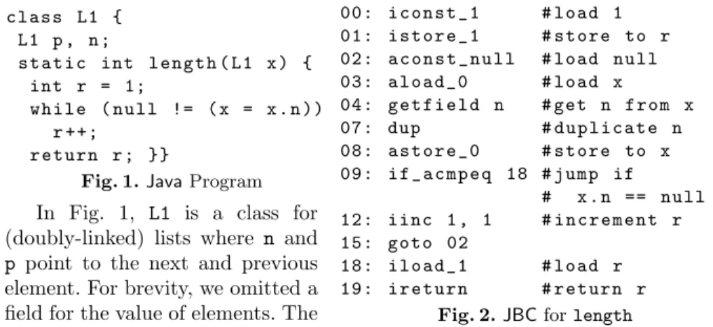
c l a s s L1 { L1 p , n ;
s t a t i c int l e n g t h ( L1 x ) { int r = 1;
w h i l e ( n u l l != ( x = x . n )) r ++;
r e t u r n r ; }}
Fig. 1.JavaProgram
00: i c o n s t _ 1 # l o a d 1 01: i s t o r e _ 1 # s t o r e to r 02: a c o n s t _ n u l l # l o a d n u l l 03: a l o a d _ 0 # l o a d x
04: g e t f i e l d n # get n f r o m x 07: dup # d u p l i c a t e n 08: a s t o r e _ 0 # s t o r e to x 09: i f _ a c m p e q 18 # j u m p if
# x . n == n u l l 12: i i n c 1 , 1 # i n c r e m e n t r 15: g o t o 02
18: i l o a d _ 1 # l o a d r 19: i r e t u r n # r e t u r n r
Fig. 2.JBCforlength In Fig. 1, L1 is a class for
(doubly-linked) lists where n and p point to the next and previous element. For brevity, we omitted a field for the value of elements. The
method lengthinitializes a variablerfor the result and traverses the list until xisnull. Fig. 2 shows the correspondingJBCobtained by theJavacompiler.
After introducing program states in Sect. 2.1, we explain how termination graphs are generated in Sect. 2.2. Sect. 2.3 shows the transformation from ter- mination graphs to TRSs. While this two-step transformation was already pre- sented in our earlier papers, here we extend it by an improved handling of cyclic objects in order to prove termination of algorithms likelengthautomatically.
2.1 Abstract States in Termination Graphs
00|x:o1|ε o1:L1(?) o1 {p,n}
Fig. 3.State A
We generate a graph of abstract states fromStates=PPos× LocVar×OpStack×Heap×Annotations, wherePPos is the set of all program positions. Fig. 3 depicts the initial state for the method length. The first three components of a state are in the first line, separated by “|”. The first component is the program position, indicated by the index of the next instruction. The second component represents the local variables as a list of references, i.e.,LocVar=Refs∗.2 To ease readability, in examples we denote local variables by names instead of numbers. So “x:o1” indicates that the 0-th local variablexhas the valueo1. The third component is the operand stackOpStack=Refs∗for temporary results ofJBCinstructions.
The empty stack is denoted byεand “o1, o2” is a stack with top elemento1. Below the first line, information about the heap is given by a function from Heap=Refs→Ints ∪ Unknown ∪ Instances ∪ {null} and by a set of annotations specifying sharing effects in parts of the heap that are not explic- itly represented. For integers, we abstract from the different types of bounded integers inJavaand consider unbounded integers instead, i.e., we cannot handle problems related to overflows. We represent unknown integers by intervals, i.e., Ints = {{x ∈ Z | a ≤ x ≤ b} | a ∈ Z∪ {−∞}, b ∈ Z∪ {∞}, a ≤ b}. For readability, we abbreviate intervals such as (−∞,∞) byZand [1,∞) by [>0].
LetClassnamescontain all classes and interfaces in the program. The values Unknown=Classnames×{?}denote that a reference points to an unknown object or to null. Thus, “o1:L1(?)” means that at address o1, we have an instance ofL1(or of its subclasses) with unknown field values or thato1isnull.
To represent actual objects, we useInstances=Classnames×(FieldIDs
→ Refs), where FieldIDs is the set of all field identifiers. To prevent ambi- guities, in general theFieldIDsalso contain the respective class names. Thus,
“o2:L1(p=o3,n=o4)” means that at address o2, we have some object of type L1whose fieldpcontains the referenceo3 and whose fieldncontainso4.
In our representation, if a state contains the referenceso1ando2, then the ob- jects reachable fromo1resp.o2 are disjoint3and tree-shaped (and thus acyclic), unless explicitly stated otherwise. This is orthogonal to the default assumptions
2 To avoid a special treatment of integers (which are primitive values inJBC), we also represent them using references to the heap.
3 An exception are references to null or Ints, since in JBC, integers are primitive values where one cannot have any side effects. So if h is the heap of a state and h(o1) =h(o2)∈Intsorh(o1) =h(o2) =null, then one can always assumeo1 =o2.
in separation logic, where sharing is allowed unless stated otherwise, cf. e.g. [32].
In our states, one can either express sharing directly (e.g., “o1:L1(p=o2,n= o1)” implies that o1 reaches o2 and is cyclic) or use annotations to indicate (possible) sharing in parts of the heap that are not explicitly represented.
The first kind of annotation is theequality annotation o=?o0, meaning that oando0 could be the same. We only use this annotation ifh(o)∈Unknownor h(o0)∈Unknown, wherehis the heap of the state. The second annotation is thejoinability annotationo%$o0, meaning thatoando0possibly have a common successor. To make this precise, let o1
→f o2 denote that the object at o1 has a field f ∈ FieldIDs with o2 as its value (i.e., h(o1) = (Cl, e) ∈ Instances and e(f) = o2). For any π = f1 . . .fn ∈ FieldIDs∗, o1 →π on+1 denotes that there exist o2, . . . , on with o1 →f1 o2 →f2 . . . f→n−1 on →fn on+1. Moreover, o1 →ε o01 iffo1 =o01. Theno%$o0 means that there could be someo00 and someπand τ such thato→π o00←τ o0, where π6=εorτ6=ε.
In our earlier papers [6, 25] we had another annotation to denote references that may point to non-tree-shaped objects. In the translation to terms later on, all these objects were replaced by fresh variables. But in this way, one cannot prove termination oflength. To maintain more information about possibly non- tree-shaped objects, we now introduce two newshape annotations o♦ando FI
instead. The non-tree annotation o♦ means that o might be not tree-shaped.
More precisely, there could be a referenceo0witho→π1 o0 ando→π2 o0 whereπ1 is no prefix ofπ2and π2 is no prefix ofπ1. However, these two paths fromotoo0 may not traverse any cycles (i.e., there are no prefixesτ1, τ2ofπ1or ofπ2where τ1 6=τ2, but oτ→1 o00 and oτ→2 o00 for some o00). The cyclicity annotation o FI
means that there could be cycles including o or reachable from o. However, any cycle must use at least the fields in FI ⊆ FieldIDs. In other words, if o →π o0 →τ o0 for some τ 6=ε, then τ must contain all fields from FI. We often write instead of ∅. Thus in Fig. 3,o1 {p,n} means that there may be cycles reachable fromo1and that any such cycle contains at least onenand onepfield.
2.2 Constructing the Termination Graph
Our goal is to prove termination of length for all doubly-linked lists without
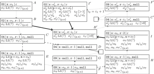
“real” cycles (i.e., there is no cycle traversing only n or only p fields). Hence, A is the initial state when calling the method with such an input list.4 From A, the termination graph in Fig. 4 is constructed by symbolic evaluation. First, iconst 1loads the constant 1 on the operand stack. This leads to a new state connected to A by an evaluation edge (we omitted this state from Fig. 4 for reasons of space). Then istore 1 stores the constant 1 from the top of the operand stack in the first local variable r. In this way, we obtain state B (in Fig. 4 we use dotted edges to indicate several steps). Formally, the constant 1 is represented by some referencei∈Refsthat is mapped to [1,1]∈Intsby the heap. However, we shortened this for the presentation and just wroter: 1.
4 The stateAis obtained automatically when generating the termination graph for a program wherelengthis called with an arbitrary such input list, cf. Sect. 5.
00|x:o1|ε o1:L1(?) o1 {p,n}
A
02|x:o1,r: 1|ε o1:L1(?) o1 {p,n}
B
04|x:o1,r: 1|o1,null o1:L1(?) o1 {p,n}
C
04|x:null,r: 1|null,null D 04|x:o2,r: 1|o2,null
o2:L1(p=o3,n=o4) o3:L1(?) o4:L1(?) o2%$o3 o2%$o4 o3%$o4 o2, o3, o4 {p,n}
E
09|x:o4,r: 1|o4,null o4:L1(?) o4 {p,n} F
09|x:null,r: 1|null,null G 09|x:o5,r: 1|o5,null o5:L1(p=o6,n=o7) o6:L1(?) o7:L1(?) o5%$o6 o5%$o7 o6%$o7 o5, o6, o7 {p,n}
H 02|x:o5,r: 2|ε
o5:L1(p=o6,n=o7) o6:L1(?) o7:L1(?) o5%$o6 o5%$o7 o6%$o7 o5, o6, o7 {p,n}
I 02|x:o01,r:i1|ε
o01:L1(?) o01 {p,n} i1: [>0]
B0
09|x:o04,r:i1|o04,null o04:L1(?) o04 {p,n}
F0
04|x:o01,r:i1|o01,null o01:L1(?) o01 {p,n} i1: [>0]
C0 02|x:o05,r:i2|ε
o05:L1(p=o06,n=o07) o06:L1(?) o07:L1(?) i2: [>1]
o05%$o06 o05%$o07 o06%$o07 o05, o06, o07 {p,n}
I0 i2=i1+ 1
Fig. 4.Termination Graph forlength
InB, we loadnulland the value ofx(i.e.,o1) on the operand stack, result- ing in C. In C, the result of getfield depends on the value ofo1. Hence, we perform a case analysis (a so-calledinstance refinement) to distinguish between the possible types ofo1 (and the case whereo1 isnull). So we obtainD where o1 isnull, andE where o1 points to an actual object of typeL1. To get single static assignments, we rename o1 to o2 in E and create fresh references o3 and o4 for its fieldspandn. We connectD andEby dashed refinement edges toC.
InE, our annotations have to be updated. Ifo1 can reach a cycle, then this could also hold for its successors. Thus, we copy {p,n} to the newly-created successors o3 and o4. Moreover, if o2 (o1 under its new name) can reach itself, then its successors might also reach o2 and they might also reach each other.
Thus, we create %$ annotations indicating that each of these references may share with any of the others. We do not have to create any equality annotations.
The annotationo2=?o3 (ando2 =?o4) is not needed because if the two were equal, they would form a cycle involving only one field, which contradicts {p,n}. Furthermore, we do not needo3=?o4, as o1 was not marked with♦.
Dends the program (by an exception), indicated by an empty box. InE,get- field nreplaceso2on the operand stack by the valueo4of its fieldn,dupdupli- cates the entry o4 on the stack, and astore 0 stores one of these entries in x, resulting inF. We removedo2ando3which are no longer used in local variables or the operand stack. To evaluateif acmpeqinF, we branch depending on the equality of the two top references on the stack. So we need aninstance refinement and createGwhere o4 isnull, and H where o4 refers to an actual object. The annotations inH are constructed fromF just asE was constructed fromC.
Gresults in a program end. InH,r’s value is incremented to 2 and we jump back to instruction 02, resulting in I. We could continue symbolic evaluation, but this would not yield a finite termination graph. Whenever two states like B andI are at the same program position, we usegeneralization (or widening [14]) to find a common representativeB0of bothBandI. By suitable heuristics,
our automation ensures that one always reaches a finite termination graph after finitely many generalization steps [8]. The values for references inB0 include all values that were possible inB orI. Sincerhad the value 1 inBand 2 inI, this is generalized to the interval [>0] inB0. Similarly, since xwasUnknownin B but a non-nulllist in I, this is generalized to anUnknownvalue inB0.
We draw instance edges (depicted by thick arrows) from B and I to B0, indicating that all concrete (i.e., non-abstract) program states represented byB orIare also represented byB0. SoBandIareinstancesofB0(writtenB vB0, IvB0) and any evaluation starting inB or Icould start inB0 as well.
FromB0 on, symbolic evaluation yields analogous states as when starting in B. The only difference is that now,r’s value is an unknown positive integer. Thus, we reachI0, wherer’s valuei2is the incremented value ofi1and the edge from F0 to I0 is labeled with “i2 =i1+ 1” to indicate this relation. Such labels are used in Sect. 2.3 when generating TRSs from termination graphs. The state I0 is similar toI, and it is again represented byB0. Thus, we can draw an instance edge from I0 to B0 to “close” the graph, leaving only program ends as leaves.
A sequence of concrete statesc1, c2, . . . is a computation path if ci+1 is ob- tained fromciby standardJBCevaluation. A computation sequence isrepresen- ted by a termination graph if there is a paths11, . . . , sk11, s12, . . . , sk22, . . .of states in the termination graph such that ci vs1i, . . . , ci vskii for alli and such that all labels on the edges of the path (e.g., “i2=i1+ 1”) are satisfied by the corre- sponding values in the concrete states. Thm. 1 shows that if a concrete statec1
is an instance of some states1in the termination graph, then every computation path starting inc1is represented by the termination graph. Thus, every infinite computation path starting inc1corresponds to a cycle in the termination graph.
Theorem 1 (Soundness of Termination Graphs).Let Gbe a termination graph, s1 some state in G, and c1 some concrete state with c1vs1. Then any computation sequencec1, c2, . . .is represented by G.
2.3 Proving Termination via Term Rewriting
From the termination graph, one can generate a TRS with built-in integers [18]
that only terminates if the original program terminates. To this end, in [25] we showed how to encode each state of a termination graph as a term and each edge as a rewrite rule. We now extend this encoding to the new annotations♦and in such a way that one can prove termination of algorithms likelength.
To encode states, we convert the values of local variables and operand stack entries to terms. References with unknown value are converted to variables of the same name. So the reference i1in stateB0 is converted to the variablei1.
Thenull reference is converted to the constantnulland for objects, we use the name of their class as a function symbol. The arguments of that function correspond to the fields of the class. So a listxof typeL1wherex.pandx.nare nullwould be converted to the termL1(null,null) ando2from stateE would be converted to the term L1(o3, o4) if it were not possibly cyclic.
In [25], we had to exclude objects that were not tree-shaped from this transla- tion. Instead, accesses to such objects always yielded a fresh, unknown variable.
To handle objects annotated with♦, we now use a simple unrolling when trans- forming them to terms. Whenever a reference is changed in the termination graph, then all its occurrences in the unrolled term are changed simultaneously in the corresponding TRS. To handle the annotation FI, now we only encode a subset of the fields of each class when transforming objects to terms. This subset is chosen such that at least one field ofFI is disregarded in the term encoding.5 Hence, when only regarding the encoded fields, the data objects are acyclic and can be represented as terms. To determine which fields to drop from the encod- ing, we use a heuristic which tries to disregard fields without read access.
In our example, all cyclicity annotations have the form {p,n} andpis never read. Hence, we only consider the field n when encoding L1-objects to terms.
Thus, o2 from stateE would be encoded as L1(o4). Now any read access to p would have to be encoded as returning a fresh variable.
For every state we use a function with one argument for each local variable and each entry of the operand stack. SoEis converted tofE(L1(o4),1,L1(o4),null). To encode the edges of the termination graph as rules, we consider the dif- ferent kinds of edges. For a chain of evaluation edges, we obtain a rule whose left-hand side is the term resulting from the first state and whose right-hand side results from the last state of the chain. So the edges fromE toF result in
fE(L1(o4),1,L1(o4),null)→fF(o4,1, o4,null).
In term rewriting [3], a rule ` → r can be applied to a term t if there is a substitution σ with `σ = t0 for some subterm t0 of t. The application of the rule results in a variant oft wheret0 is replaced byrσ. For example, consider a concrete state wherexis a list of length 2 and the program counter is 04. This state would be an instance of the abstract stateEand it would be encoded by the term fE(L1(L1(null)),1,L1(L1(null)),null). Now applying the rewrite rule above yieldsfF(L1(null),1,L1(null),null). In this rule, we can see the main termination argument: Between E and F, one list element is “removed” and the list has finite length (when only regarding then field). A similar rule is created for the evaluations that lead to stateF0, where all occurrences of 1 are replaced byi1.
In our old approach [25], the edges fromE toF would result infE(L1(o4),1, L1(o4),null)→fF(o04,1, o04,null). Its right-hand side uses the fresh variableo04in- stead ofo4, since this was the only way to represent cyclic objects in [25]. Sinceo04 could be instantiated by any term during rewriting, this TRS is not terminating.
Forrefinement edges, we use the term for the target state on both sides of the resulting rule. However, on the left-hand side, we label the outermost function symbol with the source state. So for the edge from F to H, we have the term forH on both sides of the rule, but on the left-hand side we replacefH byfF:
fF(L1(o7),1,L1(o7),null)→fH(L1(o7),1,L1(o7),null)
For instance edges, we use the term for the source state on both sides of the resulting rule. However, on the right-hand side, we label the outermost function with the target state instead. So for the edge fromItoB0, we have the term for
5 Of course, ifFI =∅, then we still handle cyclic objects as before and represent any access to them by a fresh variable.
I on both sides of the rule, but on the right-hand side we replacefI byfB0: fI(L1(o7),2)→fB0(L1(o7),2)
For termination, it suffices to convert just the (non-trivial) SCCs of the termi- nation graph to TRSs. If we do this for the only SCC B0, . . . , I0, . . . , B0 of our graph, and then “merge” rewrite rules that can only be applied after each other [25], then we obtain one rule encoding the only possible way through the loop:
fB0(L1(L1(o7)), i1)→fB0(L1(o7), i1+ 1)
Here, we used the information on the edges fromF0toI0to replacei2byi1+1.
Termination of this rule is easily shown automatically by termination provers like AProVE, although the originalJavaprogram worked on cyclic objects. However, our approach automatically detects that the objects are not cyclic anymore if one uses a suitable projection that only regards certain fields of the objects.
Theorem 2 (Proving Termination of Java by TRSs).If the TRSs result- ing from the SCCs of a termination graph Gare terminating, then G does not represent any infinite computation sequence. So by Thm. 1, the originalJBCpro- gram is terminating for all concrete states c wherecvs for some statesinG.
3 Handling Marking Algorithms on Cyclic Data
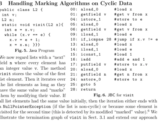
p u b l i c c l a s s L2 { int v ;
L2 n ;
s t a t i c v o i d v i s i t ( L2 x ){
int e = x . v ;
w h i l e ( x . v == e ) { x . v = e + 1;
x = x . n ; }}}
Fig. 5.JavaProgram
00: a l o a d _ 0 # l o a d x
01: g e t f i e l d v # get v f r o m x 04: i s t o r e _ 1 # s t o r e to e 05: a l o a d _ 0 # l o a d x
06: g e t f i e l d v # get v f r o m x 09: i l o a d _ 1 # l o a d e
10: i f _ i c m p n e 28 # j u m p if x . v != e 13: a l o a d _ 0 # l o a d x
14: i l o a d _ 1 # l o a d e 15: i c o n s t _ 1 # l o a d 1
16: i a d d # add e and 1
17: p u t f i e l d v # s t o r e to x . v 20: a l o a d _ 0 # l o a d x
21: g e t f i e l d n # get n f r o m x 24: a s t o r e _ 0 # s t o r e to x 25: g o t o 5
28: r e t u r n
Fig. 6.JBCforvisit We now regard lists with a “next”
field n where every element has an integer value v. The method visitstores the value of the first list element. Then it iterates over the list elements as long as they have the same value and “marks”
them by modifying their value. If
all list elements had the same value initially, then the iteration either ends with a NullPointerException (if the list is non-cyclic) or because some element is visited for the second time (this is detected by its modified “marked” value).6We illustrate the termination graph ofvisit in Sect. 3.1 and extend our approach in order to prove termination of such marking algorithms in Sect. 3.2.
6 While termination of visit can also be shown by the technique of Sect. 4 which detects whether an element is visited twice, the technique of Sect. 4 fails for analogous marking algorithms on graphs which are easy to handle by the approach of Sect. 3, cf. Sect. 5. So the techniques of Sect. 3 and 4 do not subsume each other.
05|x:o1,e:i1|ε o1:L2(?) i1:Z o1
A
06|x:o1,e:i1|o1
o1:L2(?) i1:Z o1
B
06|x:null,e:i1|null C
06|x:o2,e:i1|o2
o2:L2(v=i2,n=o3) o3:L2(?) i1:Z i2:Z o2,o3 o2%$o3 o2=?o3
D 06|x:o2,e:i1|o2
o2:L2(v=i2,n=o3) o3:L2(?) i1:Z i2:Z o2,o3 o2%$o3
E 06|x:o2,e:i1|o2
o2:L2(v=i2,n=o2) i1:Z i2:Z
F
10|x:o2,e:i1|i1, i2 o2:L2(v=i2,n=o3) o2%$o3 o3:L2(?) i1:Z i2:Z o2,o3
G 05|x:o2,e:i1|ε
o2:L2(v=i4,n=o2) i3:Z K
10|x:o2,e:i1|i1, i2
o2:L2(v=i2,n=o3) o2%$o3
o3:L2(?) i1:Z i2:Z o2,o3
H 10|x:o2,e:i1|i1, i1
o2:L2(v=i1,n=o3) o3:L2(?) i1:Z o2,o3 o2%$o3
I
10|x:o2,e:i1|i1, i2 o2:L2(v=i2,n=o2) i1:Z i2:Z
L
05|x:o3,e:i1|ε o3:L2(?) i1:Z o3
J
i1=i2 i4=i1+1
i16=i2
i16=i2 i1=i2
i3=i1+1
Fig. 7.Termination Graph forvisit
3.1 Constructing the Termination Graph
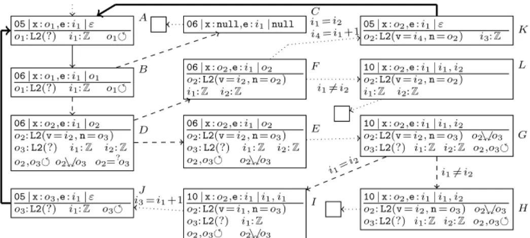
When callingvisitfor an arbitrary (possibly cyclic) list, one reaches stateAin Fig. 7 after one loop iteration by symbolic evaluation and generalization. Now aload 0loads the valueo1ofxon the operand stack, yielding state B.
To evaluate getfield v, we perform an instance refinement and create a successor C whereo1 isnull and a successorD where o1 is an actual instance ofL2. As in Fig. 4, we copy the cyclicity annotation too3and allowo2ando3to join. Furthermore, we addo2=?o3, sinceo2 could be a cyclic one-element list.
InC, we end with aNullPointerException. Before accessingo2’s fields, we have to resolve all possible equalities. We obtain E and F by an equality re- finement, corresponding to the cases o2 6=o3 and o2 = o3. F needs no anno- tations anymore, as all reachable objects are completely represented in the state.
InEwe evaluategetfield, retrieving the valuei2of the fieldv. Then we load e’s value i1 on the operand stack, which yields G. To evaluateif icmpne, we branch depending on the inequality of the top stack entries i1 andi2, resulting inH andI. We label the refinement edges with the respective integer relations.
InI, we add 1 toi1, creatingi3, which is written into the fieldvofo2. Then, the field n of o2 is retrieved, and the obtained reference o3 is written into x, leading toJ. AsJ is a renaming ofA, we draw an instance edge fromJ toA.
The states following F are analogous, i.e., when reaching if icmpne, we create successors depending on whetheri1=i2. In that case, we reachK, where we have written the new valuei4=i1+ 1 into the fieldvofo2. SinceK is also an instance ofA, this concludes the construction of the termination graph.
3.2 Proving Termination of Marking Algorithms
To prove termination of algorithms likevisit, we try to find a suitablemarking propertyM ⊆Refs×States. For every stateswith heaph, we have (o, s)∈M ifois reachable7insand ifh(o) is an object satisfying a certain property. We add
7 Here, a referenceoisreachable in a states ifs has a local variable or an operand stack entryo0 such thato0→π ofor someπ∈FieldIDs∗.
a local variable namedcM to each state which counts the number of references in M. More precisely, for each concrete stateswith “cM :i” (i.e., the value of the new variable is the reference i), h(i)∈Ints is the singleton set containing the number of references owith (o, s)∈M. For any abstract states with “cM :i”
that represents some concrete states0(i.e.,s0 vs), the intervalh(i) must contain an upper bound for the number of referenceso with (o, s0)∈M.
In our example, we consider the propertyL2.v=i1, i.e.,cM counts the refer- ences toL2-objects whose fieldvhas valuei1. As the loop invisitonly continues if there is such an object, we havecM >0. Moreover, in each iteration, the field vof someL2-object is set to a valuei3 resp.i4which isdifferent fromi1. Thus, cM decreases. We now show how to find this termination proof automatically.
To detect a suitable marking property automatically, we restrict ourselves to properties “Cl.f./ i”, whereClis a class,fa field inCl,ia (possibly unknown) integer, and./ an integer relation. Then (o, s)∈M iffh(o) is an object of type Cl(or a subtype ofCl) whose fieldfstands in relation./ to the valuei.
The first step is to find some integer referenceithat is never changed in the SCC. In our example, we can easily infer this fori1 automatically.8
The second step is to findCl, f, and ./ such that every cycle of the SCC contains some state where cM > 0. We consider those states whose incoming edge has a label “i ./ . . .” or “. . . ./ i”. In our example, I’s incoming edge is labeled with “i1=i2” and when comparingi1 and i2 inG, i2 was the value of o2’s fieldv, whereo2is anL2-object. This suggests the marking property “L2.v
= i1”. Thus, cM now counts the references to L2-objects whose fieldv has the valuei1. So the cycleA, . . . , E, . . . Acontains the stateI with cM >0 and one can automatically detect thatA, . . . , F, . . . , Ahas a similar state withcM >0.
In the third step, we addcM as a new local variable to all states of the SCC.
For instance, in Ato G, we add “cM :i” to the local variables and “i: [≥0]”
to the knowledge about the heap. The edge fromGtoI is labeled with “i >0”
(this will be used in the resulting TRS), and inIwe know “i: [>0]”. It remains to explain how to detect changes ofcM. To this end, we use SMT solving.
A counter for “Cl.f./ i” can only change when a new object of typeCl(or a subtype) is created or when the fieldCl.fis modified. So whenever “new Cl”
(or “new Cl0” for some subtype Cl0) is called, we have to consider the default valuedfor the fieldCl.f. If the underlying SMT solver can prove that¬d ./ i is a tautology, thencM can remain unchanged. Otherwise, to ensure thatcM is an upper bound for the number of objects inM,cM is incremented by 1.
If aputfieldreplaces the valueuin Cl.fbyw, we have three cases:
(i) Ifu ./ i∧ ¬w ./ iis a tautology, thencM may be decremented by 1.
(ii) Ifu ./ i↔w ./ iis a tautology, thencM remains the same.
(iii) In the remaining cases, we incrementcM by 1.
In our example, betweenI andJ one writesi3 to the fieldvof o2. To find out howcM changes fromItoJ, we create a formula containing all information on the edges in the path up to now (i.e., we collect this information by going
8 Due to our single static assignment syntax, this follows from the fact that at all instance edges,i1 is matched toi1.
backwards until we reach a state like Awith more than one predecessor). This results in i1 = i2∧i3 = i1+ 1. To detect whether we are in case (i) above, we check whether the information in the path implies u ./ i∧ ¬w ./ i. In our example, the previous valueuofo2.visi1 and the new valuewisi3. Any SMT solver for integer arithmetic can easily prove that the resulting formula
i1=i2∧i3=i1+ 1 → i1=i1∧ ¬i3=i1
is a tautology (i.e., its negation is unsatisfiable). Thus, cM is decremented by 1 in the step fromItoJ. Since inI, we had “cM :i” with “i: [>0]”, inJ we have
“cM : i0” with “i0 : [≥ 0]”. Moreover, we label the edge fromI to J with the relation “i0 =i−1” which is used when generating a TRS from the termination graph. Similarly, one can also easily prove thatcM decreases betweenF andK.
Thm. 3 shows that Thm. 1 still holds when states are extended by counterscM.
Theorem 3 (Soundness of Termination Graphs with Counters for Marking Properties). Let G be a termination graph, s1 some state in G, c1 some concrete state with c1 vs1, and M some marking property. If we ex- tend all concrete states c with heap hby an extra local variable “cM : i” such that h(i) ={|{(o, c)∈M}|} and if we extend abstract states as described above, then any computation sequence c1, c2, . . .is represented by G.
We generate TRSs from the termination graph as before. So by Thm. 2 and 3, termination of the TRSs still implies termination of the originalJavaprogram.
Since the new counter is an extra local variable, it results in an extra argu- ment of the functions in the TRS. So for the cycle A, . . . , E, . . . A, after some
“merging” of rules, we obtain the following TRS. Here, the first rule may only be applied under theconditioni >0. ForA, . . . , F, . . . Awe obtain similar rules.
fA(. . . , i, . . .)→fI(. . . , i, . . .) |i >0 fI(. . . , i, . . .)→fJ(. . . , i−1, . . .) fJ(. . . , i0, . . .)→fA(. . . , i0, . . .)
Termination of the resulting TRS can easily be be shown automatically by stan- dard tools from term rewriting, which proves termination of the methodvisit.
4 Handling Algorithms with Definite Cyclicity
p u b l i c c l a s s L3 { L3 n ;
v o i d i t e r a t e () { L3 x = t h i s . n ; w h i l e ( x != t h i s )
x = x . n ; }}
Fig. 8.JavaProgram
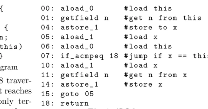
00: a l o a d _ 0 # l o a d t h i s
01: g e t f i e l d n # get n f r o m t h i s 04: a s t o r e _ 1 # s t o r e to x 05: a l o a d _ 1 # l o a d x 06: a l o a d _ 0 # l o a d t h i s
07: i f _ a c m p e q 18 # j u m p if x == t h i s 10: a l o a d _ 1 # l o a d x
11: g e t f i e l d n # get n f r o m x 14: a s t o r e _ 1 # s t o r e x 15: g o t o 05
18: r e t u r n
Fig. 9.JBCforiterate The method in Fig. 8 traver-
ses a cyclic list until it reaches the start again. It only ter- minates if by following the n
05|t:o1,x:o2|ε o1:L3(n=o2) o2:L3(?) o1,o2 o1=?o2
o1%$o2 o2 {n}99K!o1
A
07|t:o1,x:o2|o1, o2
o1:L3(n=o2) o2:L3(?) o1,o2 o1=?o2
o1%$o2 o2 {n}99K!o1
B
07|t:o1,x:o1|o1, o1 o1:L3(n=o1)
C
07|t:o1,x:o2|o1, o2 o1:L3(n=o2) o2:L3(?) o1,o2
o1%$o2 o2{n}99K!o1
D
11|t:o1,x:o2|o2
o1:L3(n=o2) o2:L3(?) o1,o2
o1%$o2 o2 {n}99K!o1
E
11|t:o1,x:o3|o3
o1:L3(n=o3)
o3:L3(n=o4) o4:L3(?) o1,o3,o4 o4=?o1
o1%$o4 o4%$o3 o4 {n}99K!o1
F 05|t:o1,x:o4|ε
o1:L3(n=o3)
o3:L3(n=o4) o4:L3(?) o1,o3,o4 o4=?o1 o1%$o4 o4%$o3 o4{n}99K!o1
G 05|t:o1,x:o4|ε
o1:L3(?) o4:L3(?) o1,o4 o4=?o1 o1%$o4 o1{n}99K! o4 o4{n}99K!o1
H
07|t:o1,x:o4|o1, o4 o1:L3(?) o4:L3(?) o1,o4 o4=?o1 o1%$o4 o1{n}99K!o4 o4{n}99K!o1
I
07|t:o1,x:o4|o1, o4
o1:L3(?) o4:L3(?) o1,o4
o1%$o4 o1
{n}99K!o4 o4 {n}99K!o1
J
11|t:o1,x:o4|o4
o1:L3(?) o4:L3(?) o1,o4
o1%$o4 o1{n}99K!o4 o4{n}99K!o1 K
11|t:o1,x:o5|o5
o1:L3(?) o5:L3(n=o6) o6:L3(?) o1,o5,o6 o6=?o1 o1%$o5 o6%$o1
o1
{n}99K!o5 o6 {n}99K!o1
L
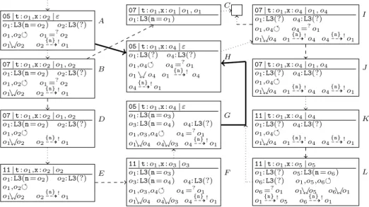
Fig. 10.Termination Graph for iterate
field, we reachnullor the first element again. We illustrateiterate’s termina- tion graph in Sect. 4.1 and introduce a newdefinite reachability annotation for such algorithms. Afterwards, Sect. 4.2 shows how to prove their termination.
4.1 Constructing the Termination Graph
Fig. 10 shows the termination graph when calling iterate with an arbitrary list whose first element is on a cycle.9 In contrast to marking algorithms like visit in Sect. 3, iterate does not terminate for other forms of cyclic lists.
StateA is reached after evaluating the first three instructions, where the value o2 of this.n10 is copied to x. In A, o1 ando2 are the first elements of the list, and o1 =? o2 allows that both are the same. Furthermore, both references are possibly cyclic and byo1%$o2,o2may eventually reacho1again (i.e.,o2
→π o1).
Moreover, we added a new annotationo2 {n}
99K!o1to indicate thato2definitely reaches o1.11 All previous annotations =?, %$, ♦, extend the set of concrete states represented by an abstract state (by allowing more sharing). In contrast, adefinite reachability annotationo99KFI ! o0withFI ⊆FieldIDsrestrictsthe set of states represented by an abstract state. Now it only represents states where o→π o0holds for someπ∈FI∗. To ensure that theFI-path fromotoo0is unique (up to cycles), FI must bedeterministic. This means that for any classCl,FI contains at most one of the fields of Clor its superclasses. Moreover, we only useo99KFI !o0 ifh(o)∈Unknownfor the heaphof the state.
InA, we load the valueso2 ando1 of xandthis on the stack. To evaluate if acmpeq in B, we need an equality refinement w.r.t.o1 =? o2. We createC
9 The initial state of iterate’s termination graph is obtained automatically when proving termination for a program whereiterateis called with such lists, cf. Sect. 5.
10In the graph, we have shortenedthistot.
11This annotation roughly corresponds tols(o2, o1) in separation logic, cf. e.g. [4, 5].