Aachen
Department of Computer Science
Technical Report
Termination Graphs for Java Bytecode
Marc Brockschmidt, Carsten Otto, Christian von Essen, J¨ urgen Giesl
ISSN 0935–3232 · Aachener Informatik-Berichte · AIB-2010-15 RWTH Aachen · Department of Computer Science · September 2010 (revised)
The publications of the Department of Computer Science of RWTH Aachen Universityare in general accessible through the World Wide Web.
http://aib.informatik.rwth-aachen.de/
Termination Graphs for Java Bytecode
⋆M. Brockschmidt, C. Otto, C. von Essen, and J. Giesl LuFG Informatik 2, RWTH Aachen University, Germany
Abstract. To prove termination ofJava Bytecode(JBC) automatically, we transformJBC to finitetermination graphs which represent all pos- sible runs of the program. Afterwards, the graph can be translated into
“simple” formalisms like term rewriting and existing tools can be used to prove termination of the resulting term rewrite system (TRS). In this paper we show that termination graphs indeed capture the semantics of JBC correctly. Hence, termination of the TRS resulting from the termi- nation graph implies termination of the originalJBCprogram.
1 Introduction
Terminationis an important property of programs. Therefore, techniques to an- alyze termination automatically have been studied for decades [6, 7, 19]. While most work focused on term rewrite systems or declarative programming lan- guages, recently there have also been many results on termination ofimperative programs (e.g., [2–4]). However, these are “stand-alone” methods which do not allow to re-use the many existing termination techniques and tools for TRSs and declarative languages. Therefore, in [14] we presented the first rewriting-based approach for proving termination of a real imperative object-oriented language, viz.Java Bytecode. Related TRS-based approaches had already proved successful for termination analysis ofHaskell andProlog[9, 15].
JBC [12] is an assembly-like object-oriented language designed as interme- diate format for the execution of Javaby aJava Virtual Machine (JVM). While there exist several static analysis techniques forJBC, we are only aware of two other automated methods to analyze termination of JBC, implemented in the toolsCOSTA[1] andJulia [17]. They transformJBC into a constraint logic pro- gram by abstracting every object of a dynamic data type to an integer denoting its path-length (i.e., the length of the maximal path of references obtained by following the fields of objects). While this fixed mapping from objects to integers leads to a very efficient analysis, it also restricts the power of these methods.
In contrast, in our approach from [14], we represent data objects not by integers, but byterms which express as much information as possible about the data objects. In this way, we can benefit from the fact that rewrite techniques can automatically generate suitable well-founded orders comparing arbitrary forms of terms. Moreover, by using TRSs with built-in integers [8], our approach is not only powerful for algorithms on user-defined data structures, but also for algorithms on pre-defined data types like integers.
⋆Supported by the DFG grant GI 274/5-3 and by the G.I.F. grant 966-116.6.
However, it is not easy to transform JBC to a TRS which is suitable for termination analysis. Therefore, we first transformJBC to so-calledtermination graphswhich represent all possible runs of theJBCprogram. These graphs handle all aspects of the programming language that cannot easily be expressed in term rewriting (e.g., side effects, cyclicity of data objects, object-orientation, etc.).
Similar graphs are also used in program optimization techniques [16].
To analyze termination of a setSof desired initial (concrete) program states, we first represent this set by a suitableabstract state. This abstract state is the starting node of the termination graph. Then this state is evaluated symbol- ically, which leads to its child nodes in the termination graph. This symbolic evaluation is repeated until one reaches states that areinstances of states that already appeared earlier in the termination graph. So while we perform consid- erably less abstraction than direct termination tools like [1, 17], we also apply suitable abstract interpretations [5] in order to obtain finite representations for all possible forms of the heap at a certain program position.
Afterwards, a TRS is generated from the termination graph whose termina- tion implies termination of the originalJBCprogram for all initial statesS. This TRS can then be handled by existing TRS termination techniques and tools.
We implemented this approach in our tool AProVE [10] and in the Inter- national Termination Competitions,1AProVEachieved competitive results com- pared toJulia and COSTA. So rewriting techniques can indeed be successfully used for termination analysis of imperative object-oriented languages likeJava.
However, [14] only introduced termination graphs informally and did not prove that these graphs really represent the semantics of JBC. In the present paper, we give a formal justification for the concept of termination graphs. Since the semantics ofJBCis not formally specified, in this paper we do not focus on fullJBC, but on JINJA Bytecode[11].2 JINJAis a small Java-like programming language with a corresponding bytecode. It exhibits the core features ofJava, its semantics is formally specified, and the corresponding correctness proofs were performed in theIsabelle/HOLtheorem prover [13]. So in the following, “JBC”
always refers to “JINJA Bytecode”. We present the following new contributions:
• In Sect. 2, we define termination graphs formally and determine how states in these graphs are evaluated symbolically (Def. 6, 7). To this end, we introduce three kinds of edges in termination graphs (Eval−→, −→,Ins −→). In contrast toRef [14], we extend these graphs to handle also method calls and exceptions.
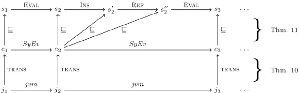
• In Sect. 3, we prove that on concrete states, our definition of “symbolic evaluation” is equivalent to evaluation inJBC (Thm. 10). As illustrated in Fig. 1, there is a mapping trans from JBC program states to our notion of concrete states. Then, Thm. 10 proves that if a program state j1 of a JBC program is evaluated to a state j2 (i.e., j1
−→jvm j2), thentrans(j1) is evaluated to trans(j2) using our definitions of “states” and of “symbolic
1 Seehttp://www.termination-portal.org/wiki/Termination_Competition.
2 For the same reason, the correctness proof for the termination technique of [17] also regarded a simplified instruction set similar toJINJAinstead of fullJBC.
s1 s2 s′2 s′′2 s3 . . .
c1 c2 c3 . . .
j1 j2 j3 . . .
}
Thm. 11}
Thm. 10Eval Ins Ref Eval
SyEv SyEv
jvm jvm
⊑ ⊑ ⊑ ⊑ ⊑
trans trans trans
Fig. 1.Relation between evaluation inJBC and paths in the termination graph evaluation” from Sect. 2 (i.e.,trans(j1)SyEv−→ trans(j2)).
• In Sect. 4, we prove that our notion of symbolic evaluation forabstractstates correctly simulates the evaluation of concrete states. More precisely, let c1
be a concrete state which can be evaluated to the concrete state c2 (i.e., c1
SyEv−→ c2). Then Thm. 11 states that if the termination graph contains an abstract state s1 which represents c1 (i.e.,c1 is an instance ofs1, denoted c1 ⊑ s1), then there is a path from s1 to another abstract state s2 in the termination graph such thats2 representsc2(i.e.,c2⊑s2).
Note that Thm. 10 and 11 imply the “soundness” of termination graphs, cf.
Cor. 12: Suppose there is an infiniteJBC-computationj1
−→jvm j2
jvm−→. . .wherej1
is represented in the termination graph (i.e., there is a states1in the termination graph withtrans(j1) =c1⊑s1). Then by Thm. 10 there is an infinite symbolic evaluationc1
SyEv−→ c2
SyEv−→ . . . , wheretrans(ji) =ci for alli. Hence, Thm. 11 implies that there is an infinite so-called computation path in the termination graph starting with the node s1. As shown in [14, Thm. 3.7], then the TRS resulting from the termination graph is not terminating.
2 Constructing Termination Graphs
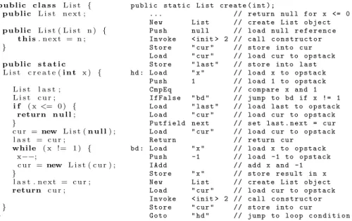
To illustrate termination graphs, we regard the methodcreatein Fig. 2.Listis a data type whosenextfield points to the next list element and we omitted the fields for the values of list elements to ease readability. The constructorList(n) creates a new list object withnas its tail. The methodcreate(x)first ensures thatxis at least 1. Then it creates a list of lengthx. In the end, the list is made cyclic by letting thenextfield of the last list element point to the start of the list. The methodcreateterminates asxis decreased until it is 1.
After introducing our notion ofstatesin Sect. 2.1, we describe the construc- tion of termination graphs in Sect. 2.2 and explain theJBCprogram of Fig. 2 in parallel. Sect. 2.3 formally defines symbolic evaluation and termination graphs.
2.1 States
The nodes of the termination graph areabstract states which represent sets of
p u b lic c l a s s L i s t { p u b lic L i s t n e x t ;
p u b lic L i s t ( L i s t n ) { t h i s. n e x t = n ; }
p u b lic s t a t i c
L i s t c r e a t e (i n t x ) {
L i s t l a s t ; L i s t c u r ; i f ( x<= 0 ) {
return n u l l; }
c u r =new L i s t (n u l l) ; l a s t = c u r ;
while ( x != 1 ) { x−−;
c u r =new L i s t ( c u r ) ; }
l a s t . n e x t = c u r ; return c u r ;
} }
public static List create ( int );
... // return null for x <= 0
New List // create List object
Push null // load null r e f e r e n c e Invoke < init > 2 // call c o n s t r u c t o r Store " cur " // store into cur Load " cur " // load cur to opstack Store " last " // store into last hd : Load " x " // load x to opstack
Push 1 // load 1 to opstack
CmpEq // compare x and 1
IfFalse " bd " // jump to bd if x != 1 Load " last " // load last to opstack Load " cur " // load cur to opstack Putfield next // set last . next = cur Load " cur " // load cur to opstack
Return // return cur
bd : Load " x " // load x to opstack
Push -1 // load -1 to opstack
IAdd // add x and -1
Store " x " // store result in x
New List // create List object
Load " cur " // load cur to opstack Invoke < init > 2 // call c o n s t r u c t o r Store " cur " // store into cur
Goto " hd " // jump to loop c o n d i t i o n
Fig. 2.Java Codeand a correspondingJINJA Bytecodefor the methodcreate concrete states, using a formalization which is especially suitable for a translation into TRSs. Our approach is restricted to verified sequentialJBCprograms with- out recursion. To simplify the presentation in the paper, as inJINJA, we exclude floating point arithmetic, arrays, and static class fields. However, our approach can easily be extended to such constructs and indeed, our implementation also handles such programs. We define the set of all states as
States= (ProgPos×LocVar×OpStack)∗×
({⊥} ∪References)×Heap×Annotations. CmpEq|x:i1,l:o1,c:o1|i2, i1
i1= [1,∞) i2= [1,1]
o1=List(next=null) Fig. 3.Abstract state
Consider the state in Fig. 3. Its first compo- nent is the program position (fromProgPos). In the examples, we represent it by the next program instruction to be executed (e.g., “CmpEq”).
The second component are the local variables that have a defined value at the current program position, i.e., LocVar = References∗. References are addresses in the heap, where we also have null∈ References. In our representation, we do not store primitive values directly, but indirectly using references to the heap.
In examples we denote local variables by names instead of numbers. Thus,
“x:i1,l:o1,c:o1” means that the value of the 0th local variablexis a reference i1 for integers and the 1st and 2nd local variables l and c both reference the addresso1. So different local variables can point to the same address.
The third component is the operand stack thatJBCinstructions operate on, i.e.,OpStack =References∗. The empty operand stack is denoted “ε” and
“i2, i1” denotes a stack with top elementi2and bottom elementi1.
In contrast to [14], we allowseveralmethod calls and a triple from (ProgPos
×LocVar×OpStack) is just one frame of the call stack. Thus, an abstract state may contain a sequence of such triples. If a method calls another method, then a new frame is put on top of the call stack. This frame has its own program counter, local variables, and operand stack. Consider the state in Fig. 4, where
Load "this"|t:o1,n:null|ε Store "cur"|x:i1|ε
i1= [1,∞)
o1=List(next=null) Fig. 4.State with 2 frames
the Listconstructor was called. Hence, the top frame on the call stack corresponds to the first statement of this constructor method. The lower frame corresponds to the statementStore "cur"
in the method create. It will be executed when the constructor in the top frame has finished.
The component from ({⊥} ∪References) in the definition of States is used for exceptions and will be explained at the end of Sect. 2.2. Here,⊥means that no exception was thrown (we omit⊥in examples to ease readability).
We write the first three components of a state in the first line and separate them by “|”. The fourth componentHeapis written in the lines below. It con- tains information about the values ofReferences. We represent it by a partial function, i.e.,Heap=References →Unknown ∪Integers ∪ Instances. The values in Unknown =Classnames×{?} represent tree-shaped (and thus acyclic) objects where we have no information except the type.Classnames are the names of all classes and interfaces. For example, “o3=List(?)” means that the object at addresso3 isnullor of typeList(or a subtype ofList).
We represent integers as possibly unbounded intervals, i.e. Integers = {{x∈ Z | a ≤x≤ b} | a ∈Z∪ {−∞}, b ∈ Z∪ {∞}, a ≤b}. So i1 = [1,∞) means that any positive integer can be at the address i1. Since current TRS termination tools cannot handle 32-bit int-numbers as in real Java, we treat intas the infinite set of all integers (this is done in JINJAas well).
To representInstances(i.e., objects) of some class, we describe the values of their fields, i.e.,Instances =Classnames×(FieldIDs→References). To prevent ambiguities, in general the FieldIDsalso contain the respective class names. So “o1 =List(next=null)” means that at the addresso1, there is a Listobject and the value of its fieldnextisnull. For all (cl, f)∈Instances, the functionf is defined for all fields of the classcl and all of its superclasses.
All sharing information must be explicitly represented. If an abstract state scontains the non-nullreferenceso1, o2 and does not mention that they could be sharing, thens only represents concrete states where o1 and the references reachable fromo1 are disjoint fromo2and the references reachable fromo2.
Sharing or aliasing for concrete objects can of course be represented easily, e.g., we could have o2 =List(next=o1) which means thato1 and o2 do not point to disjoint parts of the heap h (i.e., they join). But to represent such concepts for unknown objects, we use three kinds of annotations. Annotations are only built for referenceso6=nullwithh(o)∈/Integers.
Equality annotations like “o1 =? o2” mean that the addresses o1 and o2
could be equal. Here the value of at least one ofo1 ando2 must be Unknown. To represent states where two objects “may join”, we usejoinability annotations
“o1%$o2”. We say thato′ is adirect successorofoin a states(denotedo→so′)
iff the object at addressohas a field whose value is o′. Then “o1%$o2” means that if the value ofo1 is Unknown, then there could be an o with o1 →+s o and o2 →∗s o, i.e., o is a proper successor of o1 and a (possibly non-proper) successor ofo2. Note that%$is symmetric,3 so “o1%$o2” also means that ifo2
isUnknown, then there could be an o′ with o1 →∗s o′ and o2 →+s o′. Finally, we use cyclicity annotations “o!” to denote that the object at addresso is not necessarily tree-shaped (so in particular, it could be cyclic).4
2.2 Termination Graphs, Refinements, and Instances
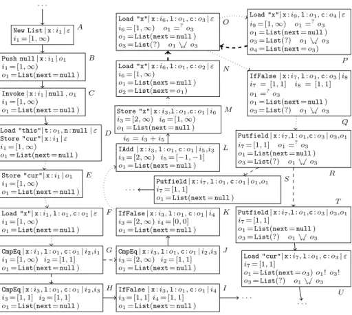
To build termination graphs, we begin with an abstract state describing all concrete initial states. In our example, we want to know whether all calls of create terminate. So in the corresponding initial abstract state, the value of xis not an actual integer, but (−∞,∞). After symbolically executing the first JBC instructions, one reaches the instruction “New List”. This corresponds to stateAin Fig. 5 where the value ofxis from [1,∞).
We can evaluate “New List” without further information aboutxand reach the nodeBvia anevaluation edge. Here, a newListinstance was created at ad- dresso1 in the heap ando1 was pushed on the operand stack. “New List” does not execute the constructor yet, but just allocates the needed memory and sets all fields to default values. Thus, thenextfield of the new object is set tonull.
“Push null” pushesnullon the operand stack. The elementsnullando1
on the stack are the arguments for the constructor <init> 2 that is invoked, where “2” means that the constructor with two parameters (nandthis) is used.
This leads toD, cf. Fig. 4. In the top frame, the local variablesthis(abbre- viatedt) andnhave the valueso1andnull. In the second frame, the arguments that were passed to the constructor were removed from the operand stack.
We did not depict the evaluation of the constructor and continue with state E, where the control flow has returned tocreate. So dotted arrows abbreviate several steps. Our implementation of<init> returns the newly created object as its result. Therefore,o1has been pushed on the operand stack inE.
Evaluation continues to node F, storing o1 in the local variables cur and last(abbreviatedcandl). InF one starts with checking the condition of the whileloop. To this end,x and the number 1 are pushed on the operand stack and the instructionCmpEqin stateGcompares them, cf. Fig. 3.
We cannot directly continue the symbolic evaluation, because the control flow depends on the value of the numberi1in the variablex. So werefine the infor- mation by an appropriate case analysis. This leads to the statesH andJ where x’s value is from [1,1] resp. [2,∞). We call this stepinteger refinementandGis connected toH andJ byrefinement edges (denoted by dashed edges in Fig. 5).
3 Since both “=?” and “%$” are symmetric, we do not distinguish between “o1 =? o2” and “o2 =? o1” and we also do not distinguish between “o1 %$ o2” and “o2 %$ o1”.
4 It is also possible to use an extended notion of annotations which also include sets ofFieldIDs. Then one can express properties like “omay joino′ by using only the fieldnext” or “omay only have a non-tree structure if one usesboth fieldsnextand prev” (such annotations can be helpful to analyze algorithms on doubly-linked lists).
. . .
New List|x:i1|ε i1= [1,∞)
A
Push null|x:i1|o1
i1= [1,∞)
o1=List(next=null) B
Invoke|x:i1|null, o1 i1= [1,∞)
o1=List(next=null) C
Load "this"|t:o1,n:null|ε Store "cur"|x:i1|ε i1= [1,∞)
o1=List(next=null) D
Store "cur"|x:i1|o1
i1= [1,∞)
o1=List(next=null) E
Load "x"|x:i1,l:o1,c:o1|ε i1= [1,∞)
o1=List(next=null) F
CmpEq|x:i1,l:o1,c:o1|i2,i1
i1= [1,∞) i2= [1,1]
o1=List(next=null) G
CmpEq|x:i3,l:o1,c:o1|i2,i3 i3= [1,1] i2= [1,1]
o1=List(next=null)
H IfFalse|x:i3,l:o1,c:o1|i4
i3= [1,1]i4= [1,1]
o1=List(next=null) I
. . . CmpEq|x:i3,l:o1,c:o1|i2,i3
i3= [2,∞) i2= [1,1]
o1=List(next=null) J IfFalse|x:i3,l:o1,c:o1|i4
i3= [2,∞)i4= [0,0]
o1=List(next=null) K IAdd|x:i3,l:o1,c:o1|i5,i3
i3= [2,∞) i5= [−1,−1]
o1=List(next=null) L Store "x"|x:i3,l:o1,c:o1|i6
i3= [2,∞) i6= [1,∞) o1=List(next=null)
M Load "x"|x:i6,l:o1,c:o2|ε i6= [1,∞)
o1=List(next=null) o2=List(next=o1)
N Load "x"|x:i6,l:o1,c:o3|ε i6= [1,∞) o1=?o3
o1=List(next=null) o3=List(?) o1%$o3
O
Load "x"|x:i9,l:o1,c:o4|ε i9= [1,∞) o1=?o3
o1=List(next=null) o3=List(?) o1%$o3
o4=List(next=o3) P IfFalse|x:i7,l:o1,c:o3|i8
i7 = [1,1] i8 = [1,1]
o1=?o3
o1=List(next=null) o3=List(?) o1%$o3
Q Putfield|x:i7,l:o1,c:o3|o3,o1 i7= [1,1] o1=?o3
o1=List(next=null) o3=List(?) o1%$o3
R Putfield|x:i7,l:o1,c:o1|o1,o1
i7= [1,1]
o1=List(next=null)
S . . .
Putfield|x:i7,l:o1,c:o3|o3,o1
i7= [1,1]
o1=List(next=null) o3=List(?) o1%$o3
T
Load "cur"|x:i7,l:o1,c:o3|ε i7= [1,1]
o1=List(next=o3)o1!o3! o3=List(?) o1%$o3
U . . .
i6=i3+i5
Fig. 5.Termination graph forcreate
To define integer refinements, for any s ∈ States, let s[o/o′] be the state obtained fromsby replacing all occurrences of the referenceoin instance fields, the exception component, local variables, and on the operand stacks byo′. By s+{o7→vl}we denote a state which results fromsby removing any information about o and instead the heap now maps o to the value vl. So in Fig. 5, J is (G+{i37→[2,∞)})[i1/i3]. We only keep information on those references in the heap that are reachable from the local variables and the operand stacks.
Definition 1 (Integer refinement).Lets∈States wherehis the heap ofs and leto∈References withh(o) =V ⊆Z. LetV1, . . . , Vn be a partition ofV (i.e.,V1∪. . .∪Vn =V) withVi∈Integers. Moreover,si= (s+{oi7→Vi})[o/oi] for fresh referencesoi. Then {s1, . . . , sn} is an integer refinementof s.
In Fig. 5, evaluation of CmpEqcontinues and we pushTrue resp.False on the operand stack leading to the nodesI and K. To simplify the presentation, in the paper we represent the BooleansTrueandFalseby the integers 1 and 0.
InI andK, we can then evaluate theIfFalseinstruction.
From K on, we continue the evaluation by loading the value ofx and the constant−1 on the operand stack. InL, IAddadds the two topmost stack ele- ments. To keep track of this, we create a new referencei6for the result and label
the edge fromL to M by the relation between i6, i3, andi5. Such labels are used when constructing rewrite rules from the termination graph [14]. Then, the value ofi6is stored inxand the rest of the loop is executed. Afterwards in state N,curpoints to a list (at addresso2) where a new element was added in front of the original list ato1. Then the program jumps back to the instructionLoad
"x"at the label “hd” in the program, where the loop condition is evaluated.
However, evaluation had already reached this instruction in state F. So the new stateN is a repetition in the control flow. The difference betweenF andN is that inF,landcare the same, while inN,lrefers too1 andcrefers too2, where the list ato1 is the direct successor (or “tail”) of the list ato2.
To obtainfinite termination graphs, whenever the evaluation reaches a pro- gram position for the second time, we “merge” the two corresponding states (like F and N). This widening result is displayed in node O. Here, the annotation
“o1 =?o3” allows the equality of the references inlandc, as inJ. ButO also contains “o1%$o3”. Solmay be a successor ofc, as inN. We connect N toO by aninstance edge (depicted by a thick dashed line), since the concrete states described byN are a subset of the concrete states described by O. Moreover, we could also connectF to O by an instance edge and discard the states G-N which were only needed to obtain the suitably generalized stateO. Note that in this way we maintain the essential invariant of termination graphs, viz. that a node “is terminating” whenever all of its children are terminating.
To define “instance”, we first define all positionsπof references in a states, wheres|πis the reference at positionπ. A positionπisexcor a sequence starting withlvi,j orosi,j fori, j∈N(indicating the jth reference in the local variable array or the operand stack of theithframe), followed by zero or moreFieldIDs. Definition 2 (State positions SPos).Lets= (hfr0, . . . ,frni, e, h, a)be a state where each stack frame fri has the form (ppi, lvi, osi). Then SPos(s) is the smallest set containing all the following sequencesπ:
• π=lvi,j where0≤i≤n,lvi=oi,0, . . . , oi,mi,0≤j≤mi. Thens|π isoi,j.
• π=osi,j where0≤i≤n,osi=o′i,0, . . . , o′i,ki,0≤j≤ki. Thens|π iso′i,j.
• π=excif e6=⊥. Then s|π ise.
• π =π′v for some v ∈ FieldIDs and some π′ ∈SPos(s) where h(s|π′) = (cl, f)∈Instancesand wheref(v)is defined. Thens|π isf(v).
For any positionπ, letπsdenote the maximal prefix ofπsuch thatπs∈SPos(s).
We writeπ ifs is clear from the context.
In Fig. 5, F|lv0,0=i1, F|lv0,1=F|lv0,2=o1. If h is F’s heap, then h(o1) = (List, f)∈Instances, wheref(next) =null. SoF|lv0,1next=F|lv0,2next=null.
Intuitively, a state s′ is an instance of a state s if they correspond to the same program position and whenever there is a reference s′|π, then either the values represented bys′|π in the heap ofs′are a subset of the values represented bys|π in the heap of sor else, πis no position in s. Moreover, shared parts of the heap ins′ must also be shared ins. Note that sincesands′ correspond to the same position in averified JBC program, s and s′ have the same number of local variables and their operand stacks have the same size. In Def. 3, the
conditions (a)-(d) handleIntegers,null,Unknown, andInstances, whereas the remaining conditions concern equality and annotations. Here, the conditions (e)-(g) handle the case where two positionsπ, π′ ofs′ are also inSPos(s).
Definition 3 (Instance). Let s′ = (hfr′0, . . . ,fr′ni, e′, h′, a′)and s= (hfr0, . . . , frni, e, h, a), where fr′i = (pp′i, lv′i, os′i) and fri = (ppi, lvi, osi). We call s′ an instanceofs(denoteds′ ⊑s) iffppi=pp′i for alliand for allπ, π′∈SPos(s′):
(a) ifh′(s′|π)∈Integers andπ∈SPos(s), then h′(s′|π)⊆h(s|π)∈Integers. (b) ifs′|π=nullandπ∈SPos(s), thens|π =nullorh(s|π)∈Unknown. (c) ifh′(s′|π) = (cl′,?)∈Unknownandπ∈SPos(s), then
h(s|π) = (cl,?)∈Unknownand cl′ is cl or a subtype of cl .
(d) ifh′(s′|π) = (cl′, f′)∈Instances andπ∈SPos(s), then h(s|π) = (cl,?) orh(s|π) = (cl′, f)∈Instances, where cl′ must be cl or a subtype of cl . (e) ifs′|π6=s′|π′ andπ, π′ ∈SPos(s), thens|π 6=s|π′.
(f ) ifs′|π=s′|π′ andπ, π′ ∈SPos(s)where h′(s′|π)∈Instances∪Unknown, thens|π =s|π′ ors|π =?s|π′.5
(g) ifs′|π=?s′|π′ andπ, π′∈SPos(s), then s|π=?s|π′.
(h) if s′|π=s′|π′ ors′|π=?s′|π′ whereh′(s′|π)∈Instances∪Unknown and{π, π′} 6⊆SPos(s)with π6=π′, thens|π %$s|π′.
(i) ifs′|π%$s′|π′, thens|π %$s|π′. (j) ifs′|π! holds, thens|π!.
(k) if there existρ, ρ′∈FieldIDs∗ without common prefix
whereρ6=ρ′,s′|πρ=s′|πρ′, h′(s′|πρ)∈Instances∪Unknown, and({πρ, πρ′} 6⊆SPos(s) or s|πρ=?s|πρ′), thens|π!.
In Fig. 5, we haveF ⊑O andN ⊑O. Symbolic evaluation can continue in the new generalized stateO. It again leads to a node likeG, where an integer refinement is needed to continue. If the value inx is still not 1, eventually one has to evaluate the loop condition again (in nodeP). SinceP ⊑O, we draw an instance edge fromP to Oand can “close” this part of the termination graph.6 If the value inx is 1 (which is checked in stateQ), we reach state R. Here, the referenceso1and o3in landchave been loaded on the operand stack and one now has to execute thePutfieldinstruction which sets thenextfield of the object at the addresso1to o3. To find out which references are affected by this operation, we need to decide whethero1=o3holds. To this end, we perform an equality refinement according to the annotation “o1=?o3”.
Definition 4 (Equality refinement).Lets∈Stateswherehis the heap ofs and wherescontains “o=?o′”. Hence,h(o)∈Unknownorh(o′)∈Unknown.
5 For annotations concernings|πwithπ∈SPos(s), we usually do not mention that they are from theAnnotationscomponent ofs, sincesis clear from the context.
6 IfPhad not been an instance ofO, we would have performed another widening step and created a new node which is more general thanOandP. By a suitably aggressive widening strategy, one can ensure that after finitely many widening steps, one always reaches a “fixpoint”. Then all states that result from further symbolic evaluation are instances of states that already occurred earlier. In this way, we can automatically generate a finite termination graph for any non-recursiveJBCprogram.
W.l.o.g. let h(o) ∈ Unknown. Let s= = s[o/o′] and let s6= result from s by removing “o=?o′”. Then{s=, s6=} is an equality refinementof s.
In Fig. 5, equality refinement ofRresults inS (whereo1=o3) andT (where o16=o3 and thus, “o1=?o3” was removed). In T’s successor U, the nextfield of o1 has been set to o3. However,o1 and o3 may join due to “o1 %$ o3”. So in particular,T also represents states where o3 →+ o1. Thus, writing o3 to a field ofo1could create a cyclic data object. Therefore, all non-concrete elements in the abstracted object must be annotated with !. Consequently, our symbolic evaluation has to extend our state with “o1!” and “o3!”. FromU on, the graph construction can be finished directly by evaluating the remaining instructions.
From the termination graph, one could generate the following 1-rule TRS which describes the operations on the cycle of the termination graph.
fO(i6,List(null), o3) → fO(i6−1,List(null),List(o3)) | i6>0∧i66= 1 (1) Here we also took the condition from the states before O into account which ensures that the loop is only executed for numbersxthat are greater than 0.
As mentioned in Sect. 1, we regard TRSs where the integers and operations like “−”, “>”, “6=” are built in [8] and we represent objects by terms. So essen- tially, for any classCwithnfields we introduce ann-ary function symbolCwhose arguments correspond to the fields ofC. Hence, the objectList(next=null) is represented by the term List(null). A state like O is translated into a term fO(. . .) whose direct subterms correspond to the exception component (if it is not⊥), the local variables, and the entries of the operand stack. Hence, Rule (1) describes that in each loop iteration, the value of the 0thlocal variable decreases fromi6 toi6−1, the value of the 1st variable remains List(null), and the value of the 2ndvariable increases fromo3toList(o3). Termination of this TRS is easy to show and indeed,AProVEproves termination ofcreateautomatically.
Getfield|x:o1|o1
o1=List(?)o1! A
Getfield|x:o2|o2
o2=List(next=o3) o3=List(?) o2! o3! o2%$o3 o2=?o3
B
. . .
Getfield|x:o1|o1
o1=List(next=o1) D Getfield|x:null|null
h i C exception:o2
o2=NullPointer() E
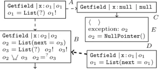
Fig. 6.Instance refinement and exceptions
Finally, we have a third kind of refinement. This instance re- finement is used if we need in- formation about the existence or the type of anUnknowninstance.
Consider Fig. 6, where in stateA we want to access thenextfield of theListobject ino1. However, we cannot evaluate Getfield, as the instance in o1 is Unknown. To refine o1, we create a successorB where the instance exists and is exactly of typeListand a stateCwhere o1 isnull.
InAthe instance may be cyclic, indicated byo1!. For this reason, the instance refinement has to add appropriate annotations toB. For example, stateD(where o1is a concrete cyclic list) is an instance of B.
InC, evaluation ofGetfieldthrows aNullPointerexception. If an excep- tion handler for this type is defined, evaluation would continue there and a refer- ence to theNullPointerobject is pushed to the operand stack. But here, no such handler exists andE reaches a program end. Here, the call stack is empty and
the exception componenteis no longer⊥, but an objecto2of typeNullPointer.
Definition 5 (Instance refinement). Let s∈States wherehis the heap of sandh(o) = (cl,?). Let cl1, . . . ,cln be all non-abstract (not necessarily proper) subtypes of cl . Then {snull, s1, . . . , sn} is an instance refinement of s. Here, snull = s[o/null] and in si, we replace o by a fresh reference oi pointing to an object of type cli. For all fieldsvi,1. . . vi,mi of cli (where vi,j has type cli,j), a new referenceoi,j is generated which points to the most general value vli,j of type cli,j, i.e., (−∞,∞)for integers and cli,j(?)for reference types. Thensi is (s+{oi 7→(cli, fi), oi,1 7→vli,1, . . . , oi,mi 7→vli,mi})[o/oi], where fi(vi,j) =oi,j
for allj. Moreover, new annotations are added in si: Ifs contained o′ %$o, we addo′=?oi,j ando′%$oi,j for all j.7 If we hado!, we also addoi,j!,oi=?oi,j, oi%$oi,j,oi,j=?oi,j′, andoi,j%$oi,j′ for allj, j′ with j6=j′.
2.3 Defining Symbolic Evaluation and Termination Graphs
To define symbolic evaluation formally, for everyJINJAinstruction, we formulate a corresponding inference rule for symbolic evaluation of our abstract states. This is straightforward for all JINJA instructions exceptPutfield. Thus, in Def. 6 we only present the rules corresponding to a simpleJINJA Bytecode instruction (Load) and to Putfield. We will show in Sect. 3 that on non-abstract states, our inference rules indeed simulate the semantics ofJINJA.
For a stateswhose topmost frame hasmlocal variables with valueso0, . . . , om, “Loadb” pushes the valueob of thebth local variable to the operand stack.
Executing “Putfieldv” in a state with the operand stacko0, o1, . . . , ok means that one wants to writeo0 to the fieldvof the object at addresso1. This is only allowed if there is no annotation “o1=?o” for anyo. Then the functionf that maps every field ofo1 to its value is updated such thatv is now mapped too0.
Putfield|. . .|o0, o1 p=List(next=o1) o1=List(next=null) o0=List(next=null)
c
. . .|. . .|ε p=List(next=o1) o1=List(next=o0) o0=List(next=null)
c′
Putfield|. . .|o0, o1 p=List(?) p%$o1 o1=List(next=null) o0=List(?)
s
. . .|. . .|ε p=List(?) p%$o1
o1=List(next=o0) o0=List(?) p%$o0
s′
⊑
⊑
Fig. 7.Putfieldand annotations
However, we may also have to update annotations when evaluat- ing Putfield. Consider the con- crete state c and the abstract statesin Fig. 7. We havec⊑s, as the connection between pand o1
in c (i.e., p→∗c o1) was replaced by “p%$o1” in s. In both states, we consider a Putfield instruc- tion which writeso0into the fieldnextofo1. Forc, we obtain the statec′where we we now also havep→∗c′ o0. However, to evaluate Putfield in the abstract states, it is not sufficient to just writeo0to the fieldnextofo1. Thenc′ would not be an instance of the resulting state s′, since s′ would not represent the connection between pand o0. Therefore, we have to add “p%$ o0” ins′. Now c′ ⊑s′ indeed holds. A similar problem was discussed for nodeU of Fig. 5, where we had to add “!” annotations after evaluatingPutfield.
7 Of course, ifcli,j and the type ofo′ have no common subtype or one of them isint, theno′=?oi,j does not need to be added.
To specify when we need such additional annotations, for any state s let o∼so′ denote that “o=?o′” or “o%$o′” is contained ins. Then we define s
as→∗s◦(=∪ ∼s), i.e.,o so′′ iff there is ano′ with o→∗so′, whereo′=o′′ or o′ ∼so′′. We drop the index “s” if s is clear from the context. For example, in Fig. 7, we havep→∗c′ o1,p→∗c′ o0 andp s′ o1,p s′ o0.
Consider a Putfieldinstruction which writes the reference o0 into the in- stance referenced by o1. After evaluation, o1 may reach any reference q that could be reached byo0 up to now. Moreover,qcannot only be reached fromo1, but from every referencepthat could possibly reach o1 up to now. Therefore, we must add “p%$q” for allp, qwithp∼o1ando0 q.
Moreover, Putfield may create new non-tree shaped objects if there is a reference p that can reach a reference q in several ways after the evaluation.
This can only happen if p q and p o1 held before (otherwise p would not be influenced by Putfield). If the new field content o0 could also reach q (o0 q), a second connection from p over o0 to q may be created by the evaluation. Then we have to add “p!” for all p for which aq exists such that p q, p o1, and o0 q.8 It suffices to do this for references pwhere the paths fromptoo1and from ptoq do not have a common non-empty prefix.
Finally, o0 could have reached a non-tree shaped object or a reference q marked with !. In this case, we have to add “p!” for allpwithp∼o1.
In Def. 6, for any mappingh, leth+{k7→d} be the function that mapsk todand everyk′ 6=k toh(k′). Forpp∈ProgPos, letpp+ 1 be the position of the next instruction. Moreover,instr(pp) is the instruction at positionpp.
Definition 6 (Symbolic evaluation SyEv−→ ). For everyJINJAinstruction, we define a corresponding inference rule for symbolic evaluation of states. We write sSyEv−→ s′ ifsis transformed tos′ by one of these rules. Below, we give the rules forLoadandPutfield(in the case where no exception was thrown). The rules for the other instructions are analogous.
s= (h(pp, lv, os),fr1, . . . ,frni,⊥, h, a)
instr(pp) =Loadb lv=o0, . . . , om os=o′0, . . . , o′k s′ = (h(pp+ 1, lv, os′),fr1, . . . ,frni,⊥, h, a) os′=ob, o′0, . . . , o′k
s= (h(pp, lv, os),fr1, . . . ,frni,⊥, h, a) instr(pp) =Putfieldv os=o0, o1, o2, . . . , ok
h(o1) = (cl, f)∈Instances acontains no annotation o1=?o s′= (h(pp+ 1, lv, os′),fr1, . . . ,frni,⊥, h′, a′) os′=o2, . . . , ok
h′=h+ (o17→(cl, f′)) f′=f + (v7→o0)
In the rule forPutfield,a′ contains all annotations in a, and in addition:
• a′ contains “p%$q” for allp, q withp∼so1 ando0 sq
• a′ contains “p!” for allpwhere p sq, p so1, o0 sq for some q, and where the paths fromptoo1 andptoqhave no common non-empty prefix.
8 This happened in stateTof Fig. 5 whereo3was written to the field ofo1. We already hado1 T o3 and o3 T o1, sinceT contained the annotation “o1 %$o3”. Hence, in the successor stateU ofT, we had to add the annotations “o1!” and “o3!”.
• ifacontains “q!” for someqwitho0→∗sqor if there areπ, ρ, ρ′ withρ6=ρ′ wheres|π=o0 ands|πρ=s|πρ′, thena′ contains “p!” for allpwithp∼so1. Finally, we define termination graphs formally. As illustrated, termination graphs are constructed by repeatedly expanding those leaves that do not cor- respond to program ends (i.e., where the call stack is not empty). Whenever possible, we evaluate the abstract state in a leaf (resulting in anevaluation edge
Eval−→). If evaluation is not possible, we use a refinement to perform a case analysis (resulting inrefinement edges−→Ref ). To obtain a finite graph, we introduce more general states whenever a program position is visited a second time in our sym- bolic evaluation and add appropriateinstance edges −→Ins . However, we require all cycles of the termination graph to contain at least one evaluation edge.
Definition 7 (Termination graph). A graph (N, E) with N ⊆ States and E⊆N× {Eval,Ref,Ins} ×N is atermination graphif every cycle contains at least one edge labelled withEvaland one of the following holds for eachs∈N:
• shas just one outgoing edge (s,Eval, s′)andsSyEv−→ s′.
• There is a refinement{s1, . . . , sn} ofsaccording to Def. 1, 4, or 5, and the outgoing edges ofsare (s,Ref, s1), . . . ,(s,Ref, sn).
• shas just one outgoing edge (s,Ins, s′)ands⊑s′.
• shas no outgoing edge and s= (ε, e, h, a).
3 Simulating JBC by Concrete States
In this section we show that if one only regards concrete states, the rules for symbolic evaluation in Def. 6 correspond to the operational semantics ofJINJA.
Definition 8 (Concrete states). Let c∈States and let hbe the heap of c.
We callcconcreteiffc contains no annotations and for allπ∈SPos(c), either c|π =null orh(c|π)∈Instances∪ {[z, z]|z∈Z}.
Def. 9 recapitulates the definition of JINJAstates from [11] in a formulation that is similar to our states. However, integers are not represented by references, there are no integer intervals, no unknown values, and no annotations.
Definition 9 (JINJA states).Let Val=Z∪References. Then we define:
JinjaStates= (ProgPos×JinjaLocVar×JinjaOpStack)∗× ({⊥} ∪References)×JinjaHeap
JinjaLocVar= Val∗ JinjaOpStack= Val∗
JinjaHeap= References→JinjaInstances JinjaInstances=Classnames×(FieldIDs→Val)
To define a functiontranswhich maps eachJINJAstate to a corresponding concrete state, we first introduce a function trVal : Val →References with trVal(o) = o for allo ∈ References. Moreover, trVal maps everyz ∈ Z to a fresh referenceoz. Later, the value ofoz in the heap will be the interval [z, z].
Now we definetrIns:JinjaInstances→Instances. For anyf :FieldIDs