Four-dimensional variational assimilation of aerosol data from in-situ and

Four-dimensional variational assimilation of aerosol data from in-situ and

remote sensing platforms

I n a u g u r a l – D i s s e r t a t i o n zur

Erlangung des Doktorgrades

der Mathematisch–Naturwissenschaftlichen Fakult¨at der Universit¨at zu K¨oln

vorgelegt von

Lars Peter Nieradzik

aus Siegen

K¨oln, 2011

Tag der letzten m¨ undlichen Pr¨ ufung: 18.10.2011

iii

Abstract

Aerosol data assimilation is mainly restricted to he ingestion of particulate

matter measurements up to 10

particle size or aerosol optical depths. The

chemistry transport model EURAD-IM of the Rhenish Institute of Environ-

mental Research (RIU) containing a sophisticated 4D-var assimilation scheme

for gas-phase constituents has been expanded by a partial adjoint of the aerosol

module MADE to enable the assimilation of species resolved aerosols data in

space and time. To set the stage for four dimensional aerosol data assimilation,

the I/O-mapping technique HDMR (High Dimensional Model Representation)

had been applied to replace the computationally demanding chemistry mecha-

nism for secondary inorganic aerosols within MADE. An adjoint of the HDMR

was constructed and the inverse transport was ensured to allow the optimisa-

tion of aerosol initial values. Furthermore, several observation operators and

their respective adjoints were built to make the processing of various types

of measurements feasible. This set of operators includes integrators for in-

situ measured

as well as particle number densities. Within the scope

of the AERO-SAM project a radiative transfer model, part of a satellite re-

trieval system SYNAER, was implemented. Its prominent feature is to provide

type resolved aerosol optical thicknesses. With construction and implementa-

tion of the adjoint radiative transfer model, EURAD-IM is able to assimilate

species resolved aerosol information. The newly formed aerosol assimilation

scheme has been applied to two dedicated episodes. First, July of 2003 was

selected when an enduring high pressure area lasted over Europe. The very

dry period allowed excessive aerosol concentrations in the troposphere. This

particular timeframe was taken to evaluate the functionality of the aerosol

assimilation system and to validate the benefit of assimilating

and espe-

cially species resolved satellite retrievals. Further, the airborne measurement

campaign ZEPTER-2 in autumn 2008 was chosen. A Zeppelin equipped with a

condensation particle counter (CPC) delivered particle number densities with

high spatial and temporal resolution. Here, the focus was set on the validation

of the assimilation system of particle number densities and its performance on

high resolved grids. In both cases initial value optimisation has been conducted

and performance of the assimilation system and its impact on the forecast have

been investigated. The studies demonstrate a considerable improvement of the

forecast quality regardless of grid resolution. Moreover, making use of aerosol

type resolved retrievals and particle number densities adds valuable informa-

tion on the aerosol properties to the model.

Kurzzusammenfassung

Die Assimilation von Aerosoldaten war bisher im Wesentlichen auf die Verwen-

dung von Messungen der Gesamtmassenkonzentrationen von Partikeln bis zu

einer bestimmten Gr¨oße und Messungen von optischer Tiefe beschr¨ankt. Das

Chemie-Transport-Modell EURAD-IM des Rheinischen Instituts f¨ur Umwelt-

forschung (RIU) enh¨alt ein hochentwickeltes vierdimensionales variationales

(4D-var) Assimilationssystem f¨ur Gasphasenspezies, das nun um eine teilwei-

se adjungierte Version des Aerosol-modells MADE erweitert wurde, um spe-

ziesaufgel¨oste Aerosolmessungen assimilieren zu k¨onnen. Vorbereitend wurde

bereits der ¨ausserst rechenzeitaufwendige Mechanismus zur L¨osung der Che-

mie der sekund¨aren anorganischen Aerosole innerhalb des MADE mithilfe ei-

nes I/O-mapping-Verfahrens ersetzt. Der resultierende Algorithmus wurde nun

adjungiert und die Funktionalit¨at des adjungierten Aerosoltransportes sicher-

gestellt. Desweiteren wurden verschiedene Beobachtungsoperatoren entwickelt

und gleichzeitig adjungiert. Dazu geh¨oren Integrationsroutinen f¨ur Massen-

konzentrationen und Anzahldichten. Im Rahmen des AERO-SAM Projektes

wurde ein Strahlungstransportmodell, Teil eines Satelliten-Retrieval-Systems,

in das Modell eingebaut. Die Besonderheit liegt darin, dass das Modell spe-

ziesaufgel¨oste aerosoloptische Tiefen liefert. Das so konstruierte Aerosolassi-

milationssystem ist auf zwei Episoden angewandt worden. Als erstes auf den

Sommer 2003, als ein langanhaltendes Hochdruckgebiet ¨uber Europa lag. Die-

se Wetterlage beg¨unstigte Waldbr¨ande und brachte stark erh¨ohte Feinstaub-

belastung mit sich. In diesem Zeitraum wurde das neue Assimilationssystem

getestet und der Nutzen der Assimilation von

insbesondere von spe-

ziesaufgel¨osten Satellitendaten untersucht. Außerdem wurde die ZEPTER-2

Messkampagne aus dem Herbst 2008 ausgew¨ahlt. Ein zur Messplatform um-

gebauter Zeppelin, der mit einem CPC (Condensation Particle Counter) aus-

gestattet war, hat r¨aumlich und zeitlich hochaufgel¨oste Partikelanzahldichten

gemessen. In dieser Episode wurde der Fokus auf die Assimilation der Anzahl-

dichten sowie der Leistung des Systems auf Modellgittern mit hoher Aufl¨osung

gerichtet. In beiden F¨allen wurde Anfangswertoptimierung durchgef¨uhrt und

das System selbst, sowie das Verm¨ogen, die Vorhersage von Aerosolen zu ver-

bessern, untersucht. Es hat sich herausgstellt, dass sich durch Assimilation von

Aerosolen eine deutliche Verbesserung der Vorhersage insgesamt erzielen l¨asst,

w¨ahrend durch die Assimilation spezies-aufgel¨oster Retrievals zus¨atzlich die

Zusammensetzung der Aerosole angepasst werden kann.

Contents

1 Introduction 1

2 Data Assimilation 5

2.1 Bayes’ Probability . . . . 6

2.2 Maximum Likelihood and Minimum Variance . . . . 6

2.3 Variational data assimilation . . . . 8

2.4 4-dimensional variational data assimilation . . . . 8

2.5 Kalman Filtering . . . 10

2.6 Summary . . . 11

3 The model system EURAD-IM 13 3.1 The EURAD-CTM . . . 15

3.1.1 Functional principle . . . 15

3.1.2 Grid specifications . . . 17

3.1.3 Initialisation . . . 18

3.2 The aerosol model MADE . . . 18

3.2.1 Size distribution . . . 20

3.2.2 Aerosol dynamics . . . 21

3.2.3 Aerosol chemistry . . . 23

3.2.4 Emissions . . . 24

3.2.5 Adjoint chemistry for secondary inorganic aerosols . . . . 24

3.3 Nesting . . . 27

3.4 Observation operators . . . 28

3.4.1 Size integrated observations . . . 29

3.4.2 SYNAER - SYNergetic AErosol Retrieval . . . 31

4 Background Error Covariance Modeling 39 4.1 Processing of Background Error Covariances . . . 40

4.1.1 The incremental formulation of the costfunction . . . 40

4.1.2 The diffusion approach . . . 41

4.2 Obtaining B . . . 42

4.2.1 Isotropic and homogeneous . . . 42

4.2.2 Ensemble calculations . . . 43

4.2.3 The NMC - method . . . 43

4.3 Current setup . . . 45

5 Episode and Campaign Simulations 47 5.1 July 2003 . . . 48

5.1.1 Episode configuration . . . 49

5.1.2 Assimilation performance . . . 51

5.1.3 Forecast performance . . . 54

5.1.4 Optimised Initial Values . . . 61

5.1.5 Summary . . . 66

5.2 ZEPTER-2 Campaign 2008 . . . 68

5.2.1 Model configuration . . . 70

5.2.2 Assimilation configuration . . . 70

5.2.3 Available observations . . . 72

5.2.4 Assimilation performance . . . 74

5.2.5 Forecast performance . . . 78

5.2.6 Optimised Particle Number Densities . . . 82

5.2.7 Summary . . . 86

6 Conclusions and Outlook 87

A Vertical Grid Structure 91

B Available ZEPTER-2 Measurements 93

CONTENTS vii

C ZEPTER-2 Flights 97

Bibliography 109

Acknowledgements 117

List of Figures

3.1 Schematic survey of the EURAD-IM model mystem . . . 14

3.2 Schematic survey of the MADE . . . 19

3.3 Log-normal distribution of number and volume density . . . 30

3.4 Footprint-H-Operator . . . 37

4.1 Schematic overview of the NMC method . . . 44

4.2 Horizontal diffusion coefficients for

. . . 45

5.1 MODIS thermal anomalies July 2003 . . . 48

5.2 Schematic overview of model runs . . . 50

5.3 Available Measurements July 2003 . . . 53

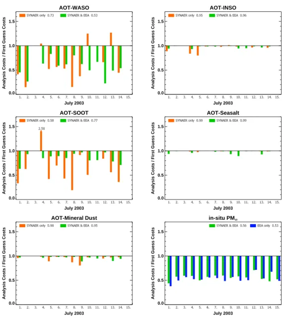
5.4 Specieswise minimisation performance July 2003 . . . 55

5.5 Relative reduction of total costs 2003 . . . 56

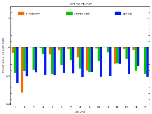
5.6 Overall relative cost reduction 2003 . . . 57

5.7 Specieswise daily forecas performance July 2003 . . . 58

5.8 In-situ

Bias and RMSE 2003 . . . 59

5.9 Error statistics for in-situ

. . . 60

5.10 Analysis and increments of accumulation mode

(WASO) . 62 5.11 Analysis field and increments of coarse mode anthropopgenic aerosols (INSO ) . . . 63

5.12 Analysis field and increments of accumulation mode elemental

carbon (SOOT ) . . . 64

5.13 Analysis field and increments of coarse mode sea salt (SEAS ) . 65

5.14 Analysis field and increments of mineral dust VSOILA . . . 66

5.15 Analysis field and increments of

. . . 67

5.16 Assimilation schedule . . . 72

5.17 Domains and in-situ measurements ZEPTER-2 . . . 73

5.18 Assimilation performance, ground and satellite observations . . 75

5.19 Assimilation performance, airborne and total . . . 76

5.20 Comparison of

and

. . . 77

5.21 Time series of

and

. . . 78

5.22 Forecast performance of

on nested grids . . . 79

5.23 Bias reduction on nested grids . . . 80

5.24 Munich-Stachus vs. Istanbul-Aksaray . . . 81

5.25 Measured

along track of flight 14 . . . 82

5.26

assimilation of Flight F14 . . . 83

5.27

analysis increments for flight F14 . . . 84

5.28

analysis increments for flight F14 (vertical cross section) 85 C.1 PND assimilation of Flight F13 . . . 98

C.2 PND assimilation of Flight F15 . . . 99

C.3 PND assimilation of Flight F16 . . . 100

C.4 PND assimilation of Flight F17 . . . 101

C.5 PND assimilation of Flight F18 . . . 102

C.6 PND assimilation of Flight F19 . . . 103

C.7 PND assimilation of Flight F20 . . . 104

C.8 PND assimilation of Flight F21 . . . 105

C.9 PND assimilation of Flight F22 . . . 106

C.10 PND assimilation of Flight F23 . . . 107

List of Tables

3.1 Standard deviations and initial diameters of the modes in MADE. 21 3.2 Aerosol species and number concentration processed in MADE

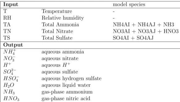
and their modal assignment. Species denominations are taken from MADE source code. . . 22 3.3 Input and output parameter and their relation to the model

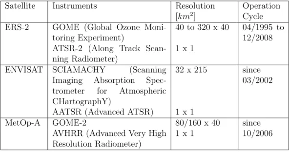
species . . . 26 3.4 List of satellite instruments the SYNAER retrieval has been

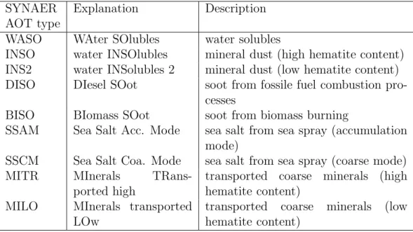
adapted to. Operational cycles taken from http://earth.esa.int . 32 3.5 SYNAER AOT types as used within retrieval and as delivered

in data product according to Holzer-Popp et al. [2008] . . . 33 3.6 Predefined mixtures within the SYNAER retrieval. . . 34 3.7 Mapping of the SYNAER AOT types onto a reduced set of

EURAD-IM SYNAER-H-Operator AOT types for the use in data assimilation. Tolerances are maximum values for which the H-Operator is valid . . . 35 3.8 List of types of SYNAER aerosol optical thicknesses and the

EURAD-IM contributing species separated by mode. See Table 3.2 for a detailed description of EURAD-IM Species . . . 36 5.1 Assimilation schedule for the episode of July 2003. Assimilation

specifications and the number of available observations for each

day of the episode. While EEA stations deliver hourly values,

each single SYNAER pixel is counted. . . . 52

5.2 List of ZEPTER-2-flights . . . 69 5.3 Configuration of the Zepter-2 nested grids. Computing time

refers to a 72-hour forecast. . . 70 5.4 Data assimilation configuration used on the nested grids during

the ZEPTER-2 campaign . . . 71 A.1 Vertical structure of the model grid . . . 91 B.1 Number of available EEA in-situ stations and total number of

P ND3

and SYNAER AOT observations for the 45 km EUR grid. 94 B.2 Number of available EEA in-situ stations and total number of

P ND3

and SYNAER AOT observations for the 15 km CEN grid. 95 B.3 Number of available EEA in-situ stations and total number of

P ND3

and SYNAER AOT observations for the 5 km ZP2 grid. 96

List of Acronyms

AATSR

Advanced ATSR

3D-var

Three-Dimensional Variational

Four-Dimensional Variational

AErosol RObotic NETwork

AERO-SAM

AEROsol characterization from Space by advanced data Assimilation into a tropospheric chemistry Model

AOD

Aerosol Optical Depth

AOT

Aerosol Optical Thickness

AVHRR

Advanced Very High Resolution Radiometer

Background Error Covariance Matrix

BLAOT

Boundary Layer Aerosol Optical Thickness

Best Linear Unbiased Estimate

CPC

Condensation Particle Counter

CTM

Chemistry Transport Model

DFD

Deutsches Fernerkundungsdatenzentrum

DFG

Deutsche Forschungsgemeinschaft German Science Foun- dation

DLR

Deutsches Zentrum f¨ ur Luft- und Raumfahrt

ECMWF

European Centre for Medium-Range Weather Forecast

EEA

European Environment Agency

EEM

EURAD Emission Model

EnKF

Ensemble Kalman Filter

ENVISAT

ENVIronmental SATellite

ERS-1/2

European Remote sensing Satellite 1 and 2

EURAD-IM

European Air Pollution Dispersion - Inverse Model

Fully Equivalent Operational Model

GOME

Global Ozone Mapping Experiment

GOME-2

second Global Ozone Monitoring Experiment

Global Positioning System

HDMR

High Dimensional Model Representation

KF

Kalman Filter

L-BFGS

Limited-Memory Broyden Fletcher Goldfarb Shanno

Modal Aerodol Dynamics model for Europe

MetOp-A

METeorological OPerational satellite-A

MIM

Mainz Isoprene Mechanism

MM5

Fifth-Generation NCAR / Penn State Mesoscale Model

MODerate-resolution Imaging Spectroradiometer

National Aeronautics and Space Administration

National Center for Atmospheric Research

National Center for Environmental Prediction

National Meteorological Center

RACM

Regional Atmospheric Chemistry Mechanism

Regional Acid Deposition Model

RIU

Rheinisches Institut f¨ ur Umweltforschung

Regional Particulate Model

RPMARES

Regional Particulate Model Aerosol REacting System

Scanning Imaging Absorption Spectrometer for Atmo-

spheric Chartography

SORGAM

Secondary ORGanic Aerosol Model

SPRINTARS

Spectral Radiation-Transport Model for Aerosol Species

SYNergistic AErosol Retrieval

UTC

Coordinated Universal Time

Volatile Organic Compounds

WRF-chem

Weather Research and Forecast (WRF) model coupled with CHEMistry (WRF-Chem)

ZEPTER-2

second ZEPpelin based Tropospheric photochemical

chemistry expERiment

CHAPTER 1

Introduction

Since the advent of numerical atmospheric modeling in the 1950ies there has been an endeavor to enhance the models’ prediction skills and to process a maximum of available information to achieve a representation of the state of the atmosphere that is as accurate as possible. The complexity of models has been rising with the increase of computational power. The spatial and tempo- ral resolution of model grids has become increasingly finer, the representation of physical processes has become more elaborate, and, in terms of chemistry transport modeling, the number of chemical compounds and, hence, reactions has become larger. But still, it is apparent that a good prediction does need a reasonable estimate to start from, a set of optimum initial values. The pro- vision of initial values by employing as much available information as possible is the traditional goal of data assimilation. It combines the new, yet mostly sparse information from observations with the physical and chemical knowl- edge of atmospheric processes encoded in the numerical models.

From numerical weather simulations (see for example Lorenc [1986]) the vari- ous techniques consequently found their way to chemistry transport modeling.

Here, the works of Elbern et al. [1997] and Elbern and Schmidt [2001] showed

the usefulness of a four dimensional variational data assimilation (4D-var) sys-

tem applied to provide both, optimised initial values as well as optimised emis-

sion factors, with EURAD-IM (EURopean Air pollution Dispersion - Inverse

Model, Ebel et al. [1993], Ebel et al. [1997]). In 1997 the ECMWF (European

Centre for Medium-Range Weather Forecast) developed the first meteorologi-

cal 4D-var system for operational use (Rabier et al. [2000]).

In the recent decade aerosols more and more came into the view of science and politics. Their impact on human health has been investigated largely, as shown by Brimblecombe and Maynard [2001] or the CAFE report by European Commission [2005]. Furthermore, the significance of aerosols concerning the earth’s radiative budget and, hence, influencing the global climate (Intergov- ernmental Panel on Climate Change [2001]) motivates efforts to get a best possible estimate of the atmospheric aerosol burden. Their impact can be di- rect, in terms of scattering, reflection, and absorption of solar light as well as the earth’s long wave radiation, the so called “direct forcing”. On the other side, aerosols act as cloud condensation nuclei (CCN) with the effect of an increased rate of cloud formation leading to an enhanced albedo. This effect is called “indirect forcing”.

Various effects of aerosols do not only depend on their physical properties but

also on their composition. Salt aerosol mainly found in coastal areas but also

induced deliberately in health resorts is said to have a positive effect on the res-

piratory system. On the other side mineral dust from volcanic eruptions may

cause serious damage to aircrafts. These very distinct effects of the different

substances an aerosol can be composed of brings up the necessity for differ-

entiated aerosol simulations. While this is already standard in many aerosol

models, there still is a lack of type resolved aerosol measurements to either

evaluate the models or to assimilate them. The first steps in 3D-var assimila-

tion of AOT into a model with evolving aerosols were accomplished by Collins

et al. [2001] using four species, sulfate, carbonaceous, mineral dust, and sea

salt. More recently, Kahnert [2009] showed the beneficial impact on aerosol

forecast by applying 3D-var on AOT in a model using seven species in four size

bins. Also, Pagowski et al. [2010] showed the valuable impact of optimised ini-

tial values by 3D-var of ground based

. This study was conducted with

MADE. Another approach with Ensemble Kalman Filtering (EnKF) was made

by Schutgens et al. [2010] using a two species parameterisation (fine and coarse

mode particles) for the assimilation of AERONET AOD (AErosol RObotic

NETwork) in the SPRINTARS model (Spectral Radiation-Transport Model

for Aerosol Species). The ECMWF is currently operating a 4D-var-scheme

with three size bins each for dust and sea salt and one size bin each for or-

ganics, black carbon, and sulfate assimilating unspecified MODIS (MODerate-

resolution Imaging Spectroradiometer) AOD (Benedetti et al. [2009]). All of

the studies mentioned above use bulk measurements for assimilation, i.e. inte-

grated values like

or AOT that give no information on the aerosol com-

position. Even more, these model setups are bound to their modeled aerosol

3

compositions, since all of them use the technique of repartitioning (reassigning the analysis to the a priori composition of aerosols). While 4D-var is able to assimilate measurements “where and when they are”, the EnKF needs to accumulate the measurement into several assimilation windows. The 3D-var approach generates new model states at one point in time. Except for the study presented by Pagowski et al. [2010] whose model has a resolution of 12 km, all simulations have been accomplished on rather coarse grids with spac- ings of 25 km and more.

So far, the inverse modeling of the physical properties of aerosols in a box model was given by Sandu et al. [2005], who presented an adjoint of the coagulation scheme, and Henze et al. [2004] who introduced an inverse mechanism for con- densational growth.

Addressing the above characteristics this study presents an assimilation sys- tem, that

•

is capable of ingesting type resolved observations,

•

can process particle properties, namely particle number densities,

•

is applicable on highly resolved grids,

•

and delivers smooth and timely coherent analysis fields as an intrinsic property of the 4D-var approach..

First of all, the proper observations need to be at hand. Besides the few so

called super sites which measure separate aerosol components like sulphate, ni-

trate, or chloride most of the available aerosol in-situ observations deliver lump

measurements that contain only the overall mass concentration of particles up

to a certain diameter, like

. Another important source of information

on atmospheric aerosols are remote sensing instruments aboard several satel-

lites which in general deliver overall aerosol optical thicknesses. Here, again,

no information on the composition of the aerosol is contained. However, the

SYNAER retrieval system (Holzer-Popp et al. [2002b]) developed at DLR-DFD

offers type resolved aerosol optical thicknesses and, thus, the opportunity to

assimilate not only AOT, but also assign it to certain species contained in

the model. Finally, this leads to a more comprehensive representation of the

atmosphere’s aerosols. As another novelty, particle number densities with a

high temporal resolution gathered during an airborne measurement campaign

were at hand.

The four dimensional variational data assimilation system for aerosols was added to the already existing foundation of a sophisticated gas-phase 4D-var system. The aerosol model MADE (Modal Aerodol Dynamics model for Eu- rope, Ackermann [1997], Ackermann et al. [1998]) was expanded by an adjoint condensation scheme. Therefore, the original condensation scheme (Friese and Ebel [2010]) was replaced by a FEOM (Fully Equivalent Operational Model, Nieradzik [2005]) based on the principle of HDMR (High Dimensional Model Representation, see Rabitz and Alis [1999]). This FEOM consists of a set of multidimensional multivariate functions which, besides being much faster in computation than its predecessor, facilitates the building of an adjoint.

Furthermore, the respective observation operators for the various observations have been built. Altogether, it proves to be a skillful tool to improve mesoscale simulation of tropospheric aerosols.

This study is organised as follows: In chapter 2 an overview is given on four dimensional variational data assimilation including a comparison with the most common data assimilation techniques. Subsequently the EURAD-IM model system and its aerosol model MADE are introduced in chapter 3 along with the newly implemented algorithms. Chapter 4 addresses the various types of aerosol related measurements which the EURAD-IM is now able to assimilate.

Furthermore, the observation-operators necessary to map from model space to

observation space and their adjoints are presented here. The application of the

aerosol assimilation system on two selected episodes is illustrated in chapter

5, along with validation results of the system and an evaluation of the impact

of optimised aerosol initial values on the forecast quality. This thesis finally

concludes in chapter 6 where a summary and an outlook on future research

options is given.

CHAPTER 2

Data Assimilation

Numerical models used in atmospheric sciences are always a simplified repro- duction of the real atmosphere. They are limited in terms of their spatial and temporal resolution and to a restrictive selection of physical and chemical pro- cesses. This is a necessary trade off between accuracy and diversity (e.g. the number of species treated) on one side and computational power limitations on the other. Numerical modeling is an initial value/boundary conditions prob- lem. Hence, the model performance will be aligned to the grade of knowledge of these. Since these conditions themselves are only modeled, i.e. the out- come of a preceeding simulation, or a fixed set of climatological average values based on long term observations or investigation of relevant data sets, they are generally far from ideal. Altogether, numerical models are limited to the knowledge encoded by their programmers in form of physical laws, chemical reactions, orographic information, and the like.

Another source of information on the state of the atmosphere are measure- ments. They can provide a detailed insight into the atmosphere’s current condition, be it on a large scale in form of satellite retrievals or be it in-situ measurements from ground based or airborne instruments. Unfortunately, this multitude of information does not directly provide the necessary initial con- ditions to the model, since they themselves underlay a variety of limitations.

First of all, their spatial distribution tends to be rather inhomogeneous and

many measurement sites are not representative for an area of the size of a

model grid cell. Often the desired species are not measured directly, e.g. satel-

lite retrievals of aerosol optical thicknesses instead of aerosol concentrations,

and, finally, they are afflicted with errors.

The techniques summarised under the concept of Data Assimilation have evolved from the desire of ”using all available information, to determine as accurately as possible the atmospheric (or oceanic) flow” as defined by Tala- grand [1997]. Data assimilation acts as an interface between the various types of information on the state of the atmosphere on one side and the knowledge of the physical and chemical processes in the atmosphere on the other. While observations of the atmosphere’s state and composition can be very exact they are limited in time and space. Models, on the other hand, deliver a continuous and smooth image of the atmosphere but are restricted to discretisation and a limited set of equations describing the major processes. To retrieve a max- imum gain of information from both these scientific tools is the goal of data assimilation.

This chapter outlines the theory of data assimilation. Furthermore, a rough survey of the various methods will be given before the variational approach, which has been applied in this work, will be described in detail. For a more comprehensive comparison of these methods see e.g. Kalnay [2003], Lahoz et al. [2010].

2.1 Bayes’ Probability

Assume, that there is a probability density function (PDF)

of the atmosphere

which can be derived, e.g. from an ensemble simulation or climatology. This is the a priori probability to simulate

if an information

on the condition is known - a measurement - and its error characteristics are available, a PDF

probability of taking a measurement

when condition

holds.

Following Bayes’ theorem, the a posteriori probability

by

p

(x

(y

(x)

p

(y) =

(y

(x)

R p

(y

)

(x

)

(2.1)

2.2 Maximum Likelihood and Minimum Vari- ance

With the further assumption that these PDFs are of Gaussian character and

being the standard deviation of

when the

2.2 Maximum Likelihood and Minimum Variance 7

true state

is given can be expressed as

(y

1

√

2πσ

−(y−x)2 2σ2

y .

(2.2)

On the other side, the likelihood of

as the true state given

is simply

Lσy

(x

(y

(2.3)

In the presence of a multitude of

measurements the overall likelihood be- comes

Lσy1,...,σ_yN

(x

) =

N

Y

i=1

√

1

2πσ

(yi−x)²

2σ2 yi

!

= 1

√

2π

(y1−x)2 2σ2

1

···−(yN−x)²

2σ2

N ,

(2.4)

the joint probability. Consequently, the maximum of 2.4 is most likely to be true value of

the logarithm is a monotonous function yields

max L_{σy1,...,σyN}

(x

)

=

const

(y

2σ

(y

2σ

!

.

(2.5)

Taking another look at Bayes’ Theorem and assuming that

(x) can be con- sidered a prior PDF of the true state in the presence of an information

(the background information, also referred to as the first guess) that also yields a Gaussian probability in the form of

(x) = 1/

2πσ

·e^{−(x0−x)2/2σ20}

one can write the a posteriori probability of 2.2 as

p

(x

(y

(x)

(y) =

N

Y

i=1

√

1 2πσ

·e⁻

(yi−x)²

2σ2 yi

!

·

1

√

2πσ

·e⁻

(x0−x)2 2σ2

x0

(2.6)

The right term in 2.2 shows that the denominator is independent of

its maximum can be obtained by maximising the numerator in an analogous

manner as in 2.5.

2.3 Variational data assimilation

Maximising 2.5 delivers the most likely state of the atmosphere

, the so called Analysis. In data assimilation this is technically done by minimising a Cost Function

1 and it contains the sum of the squares of the misfit of each of the observations and the background field to the state vector

weighted by their individual variance:

J(x) =

1 2

"

(y

2σ

+ (x

)

2σ

#

(2.7) or, as it is generally written in data assimilation:

J(x) =

1 2

h

(H(x)

R

(H(x)

B

(2.8) with the superscript

indicating the transposed of a vector, R the obser- vation or measurement error covariance matrix, and B the background error covariance matrix.

observation or forward operator. It is a mapping from the model space into the space of the observation. This can be a simple multilinear interpolation from the model grid to the location of the measurement, but might as well be as complex as a full radiative transfer model. Different types of H-operators and their properties will be discussed in section 3.4. An important property of this formulation of the cost function is, that it is minimised with respect to

stationary in time, i.e. it delivers a BLUE (Best Linear Unbiased Estimate) of the model state for one point in time. It is therefore referred to as Three Dimensional variational data assimilation (3D-var).

2.4 4-dimensional variational data assimilation

It is desirable to make use of as many measurements as possible. But these are generally distributed not only in space but also in time. To find an optimum for the state of the atmosphere at a time

(henceforth reffered to as initial time) taking into account all measurements within a certain temporal interval the costfunction 2.8 has to be modified to

J(x₀

) =

+

= 1

2

B

+ 1

2

N

X

i=1

[H (M

(x

)

)]

R

[H (M

(x

)

)]

(2.9)

2.4 4-dimensional variational data assimilation 9

where

is the model operator generating the state

at timestep

from the initial conditions

, y

is a vector containing all observations at timestep

) is now minimised to gain an optimum state

, the analysis, i.e. a BLUE of the initial conditions of the assimilation interval with respect to all observations within this interval. Minimisation is done by numerical methods, like a Conjugate Gradient or a quasi-Newton algorithm.

It is accomplished by building the gradient of

(x

) and approaching its zero.

One constraint that is made in 4D-var is that the model is assumed to be errorless over the whole interval. Only the initial values are afflicted with errors. The gradient of

) with respect to

can easily be derived from Equation 2.9 resulting in

∇^x0J^b

= B

(2.10) Quite similarly, the gradient of the observational part of the costfunction can be calculated

∇^xiJ^o

= H

R

(H(x

)

) (2.11)

here, the gradient is valid at time

but the gradient is needed for

. Now, let

be a perturbation at

= 0, then, using the model operator

from Equation 2.9 the perturbation at

=

can be defined as

δxi

:= M

(x

+

)

M

(x

) (2.12)

The tangent linear model M

is a linear approximation of the model operator

, its Jacobian. It can thus be stated that

δxi ≈

M

(δx

) (2.13)

Making use of the canonical scalar product

iui·vi

one can write a variation of

(x) as a result of

as

δJ ≈<∇^xiJ, δxi >

This way, the term of observation costs in 2.9 can be written as

=

N

X

i=0

<∇^xiJ^o, δxi >

and with the assumption that 2.13 holds this transforms to

=

N

X

i=0

<∇^xiJ^o,

M

(δx

)

(2.14)

Now, using the property

the variation of

turns to

=

N

X

i=0

<

M

(2.15) where, M

:= M

is the transpose of the tangent linear, the adjoint model.

The gradient of the observation costfunction can now be derived for

= 0 recalling 2.11

∇x0J^o

=

N

X

i=0

M

=

N

X

i=0

M

H

R

(H(x

)

) (2.16) Now, the whole costfunction with respect to the gradients at

= 0 can be summed up to

∇^x0J

=

+

= B

+

N

X

i=0

M

H

R

(H(x

)

) (2.17)

2.5 Kalman Filtering

The most sophisticated yet complex method is the Extended Kalman Filter, often referred to as the ”Gold Standard of data assimilation” (Kalnay [2003]) in contrast to the 4D-var method it delivers the analysis error covariance matrix

at every timestep

and does take into account the error produced by the model while propagating in time. According to Kalnay [2003] this can be summarised as follows: Let

be the forecasted model state at

=

propagated by the Model

from the analysis

at the preceding time-step

=

1 then the forecast can be described as

x^f_i

=

(2.18) and a forecast error covariance matrix P

gained by propagation of P

via

P

= L

P

L

+ Q

(2.19)

where L

is the Tangent Linear Model, a linear approximation of the model

at timestep

under the condition of

, and L

its transposed or so called

adjoint. Q

is a matrix representing the noise of the model, i.e. the error

inflicted by the model itself. Furthermore, H

is used in the following being

2.6 Summary 11

the linearisation of the forward operator

at the state

. Now, the analysis for timestep

can be computed by first minimising P

(t

) in

P

= (I

K

H

) P

(2.20)

and finally updating

=

+ K

y

)

(2.21) with K being the so called Kalman gain matrix that is set up after the forecast steps as

K

= P

H

R

+ H

P

H

(2.22) Equation 2.19 describes the crucial step in extended Kalman Filtering. With L being of the size of the degrees of freedom of the model (which can easily be of the order of 10

or more), the step of propagating P

in time is as costly as the same number of model forward integrations. This prohibits the use of extended Kalman Filters for common problems. Several techniques have been developed, to enhance performance by reducing model size or making reason- able assumptions, like e.g. the ensemble Kalman filter, which are described in detail in Kalnay [2003], Lahoz et al. [2010] or Daley [1991].

2.6 Summary

In operational model set-ups it is common to apply pseudo-4D data assimila- tion. That is, applying a 3D-var scheme at, for example, every full hour. This is due to computational demands of a full 4D-var system on one hand but, above all, because no adjoint model needs to be constructed or maintained.

In 4D-var assumptions have to be made about the background error covari-

ance matrix B while the extended Kalman Filter propagates the model error

in time and, thus, delivers the more complete description of the state of the

atmosphere. This is, on the other hand, not feasible for standard models due

to the immense computational effort. Also, does the 4D-var analysis deliver

a smooth and physically and chemically consistent state within the assimila-

tion window, while Kalman filtering produces perturbations through jumps

whenever an analysis step is performed.

CHAPTER 3

The model system EURAD-IM

The EURAD-IM model system has been developed on the base of the EURAD- CTM (EURopean Air pollution Dispersion - Chemistry Transport Model).

The suffix IM (Inverse Model) indicates that EURAD-CTM has been expanded by an inverse part for data assimilation purposes. The forward part of the model system - the standard forecast system - consists of three major models:

•

MM5

The Mesoscale Meteorological model 5 (Grell et al. [1994]) acts as me- teorological driver for the CTM, i.e. it delivers the meteorological fields needed like, for example, wind, relative humidity, and temperature.

•

EEM

The EURAD-Emission-Model (Memmesheimer et al. [1991]) delivers emis- sion fields taylored for the specific grid used considering diurnal cycle, day of the week, international holidays, and season.

•

CTM

The chemistry transport model (Hass [1991]; Hass et al. [1995]; Ebel et al.

[1997]) computes transport, chemical transformation, and deposition of

gas-phase and aerosol-phase species.

iterations EEM

emission rates

PREP

observations

MM5

meteorology

x x0 N

CTM

forecast initial values

emission factors

J ( x ,f )0

x x

N 0

* * J ( x ,f )0

J ( x ,f ) = min0

observations gradient

ADCTM

adjoint run cost function

minimisation

LBFGS

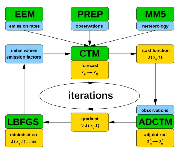
Figure 3.1: Schematic survey of the EURAD-IM model system. Explanation in the text.

The inverse model system contains three additional parts.

•

PREP

The data PREProcessor provides desired measurement data from any kind of available measurement.

•

ADCTM

Adjoints of many of the forward routines (in 4Dvar only), H-operators for the mapping between model and observation space.

•

LBFGS

The implemented minimisation algorithm that evaluates gradient and

costfunction is the Limited-memory Broyden-Fletcher-Goldfarb-Shanno

algorithm (Liu and Nocedal [1989]).

3.1 The EURAD-CTM 15

The EURAD-IM is a Eulerian model system. The chemistry is calculated on a fixed three dimensional grid and transport is simulated as fluxes through the boundaries of each grid cell. The meteorological driver MM5 and the EEM are run offline, thus, there is no feedback from the CTM. Figure 3.1 displays the calling sequence of the particluar model components and the data flow within a model simulation. A standard forecast simulation is composed of the sequential call of MM5, EEM, and CTM, though in a newer version, an online-version of the EEM is available, where emissions are calculated within the CTM. Four dimensional fields of concentrations of gas-phase and aerosol phase species are delivered as output.

An assimilation run is setup with additional featuers. First, another offline process, the PREP is run offline to provide desired observations in a proper way. Then, the CTM is run forward as in a standard forecast with the ex- ception, that the cost function is summed up over all time steps from the beginning to the end of the simulation and that the model state is stored for each time step to be recalled in the backward run. Then, a backward or ad- joint run is accomplished from the ending point to the beginning. Here, on each time step the gradients are propagated backward in time via the adjoint parts of the CTM. Here, the stored fields are used to reproduce the state of the model during the forward run. Finally, the L-BFGS minimisation algo- rithm receives a set of gradients and the scalar value of the cost function and delivers a vector of increments (this is explained in the context of the diffusion paradigm in Chapter 4). These are then added to the background values and a new iteration is started. This is repeated until either a break off criterion is met or a maximum number of iterations is reached.

The components relevant for the work presented in this thesis are explained in more detail in the following.

3.1 The EURAD-CTM

The core of the system, the CTM, simulates advection and diffusion, chemical conversion, and deposition of trace gases and aerosols in the atmosphere.

3.1.1 Functional principle

Basically, the CTM solves the following equation (Hass [1991]):

∂c_i

∂t

=

(uc

) +

(K

) +

∂t |^chem

+E

+F

+

∂t |^cloud

+

∂t |^aerosol

(3.1)

Here,

indicates the mean concentration of the species

right hand side of Equation (3.1) represent changes of concentration due to the following processes:

• ∇

(uc

): Advection, that is transport by wind, where u is the vector of wind velocity

• ∇

(K

): Turbulent diffusion, with the tensor of turbulent diffusion

• ^∂c_∂tⁱ|^chem

: Chemical conversion in the gas phase

• E_i

: Emission rates

• Fi

: Sum of the following fluxes:

–

: Flux by emissions from the surface –

: Flux by dry deposition to the surface

• ^∂c_∂tⁱ|^cloud

: Aqueous chemistry, transport in clouds and wet deposition

• ^∂c_∂tⁱ|aerosol

: Aerosol chemistry processed in MADE

A so called operator splitting is applied (see McRae et al. [1982]) on the pro- cesses of dynamics. The processes of advection and diffusion are split and symmetrically arranged around the solver modules for gas-phase chemistry and aerosol dynamics following

x_i

(t + ∆t) =

(t) (3.2) with

denoting the model state, that is a concentration or mixing ratio, of species

the time step, ∆t length of a time step,

the advection module in horizontal and vertical direction, respectively,

the vertical diffusion,

the gas-phase chemistry solver, and

the aerosol dynamics module MADE.

Here, the

and

are applied for one half of the model’s timestep before and one half after chemistry and aerosol dynamics (see Hass [1991]).

The current EURAD-CTM uses the Bott upstream advection-scheme Bott [1989] of fourth order in both, vertical and horizontal direction. An adjoint of this advection-scheme is available. The inverse model integration of the gradient is then represented by

x^∗_i

(t

∆t) =

(t) (3.3)

where

(t) is the adjoint variable

at time

superscript

denotes the adjoint of the affected operator.

3.1 The EURAD-CTM 17

Originally, the EURAD-CTM was built up around the RADM (Regional Acid Deposition Model, Chang et al. [1987]). In these studies the Chemistry is repre- sented by the RACM (Regional Atmospheric Chemistry Mechanism, Stockwell et al. [1997]) and an extension based on the MIM (Mainz Isoprene Mecha- nism, Geiger et al. [2003]). Moreover, it contains the sophisticated aerosol model MADE described in more detail later in this chapter. The description of the adjoint model concerning gas-phase has already been described in detail in Elbern and Schmidt [1999], Elbern et al. [2000], and Elbern and Schmidt [2001] and emission factor optimisation has been accomplished and analysed in Strunk [2006] and Elbern et al. [2007]. Therefore, these parts will not be treated here.

3.1.2 Grid specifications

The grid of EURAD-CTM is a Lambert conformal conic projection with an equidistant rectangular horizontal spacing. The state variables are represented in a way following the Arakawa C-Grid definition (Arakawa and Lamb [1977]) and the layers are determined by terrain following sigma coordinates that are defined as

σk

=

pbot−ptop

(3.4) with

being the layer number and

the pressure at the surface, layer

the vertical layers is given in appendix A.

Lateral boundary conditions

The vertical grid defined by Equation 3.4 are also used to represent the con- ditions at the lateral boundaries, the ring of the outermost grid cells of the model’s mother domain. From measurements and climatological information a fixed set of boundary values has been derived depending on layer and latitude.

In the case of inflow the flux into the model domain is given by

Fb

= u

(3.5)

where u

is the wind velocity perpendicular to the boundary. On out flowing conditions a constant advection through the two two grid boxes is applied, i.e.

fluxes into and out of the boundary grid cell are equal. This is done to avoid

reflection of out flowing waves. The lateral boundaries are located in regions

of low pollution. The area of interest should be chosen in a certain distance to

the boundaries to avoid a strong influence on the simulation (see Schell [1996]

for a detailed description).

Vertical boundary conditions

The top boundary of the CTM is set fix at 100

fluxes at the top of the top layer are set to zero. Thus, it functions as a lid.

The bottom boundary is the earth’s surface and here the boundary conditions are represented by deposition and emission, the terms

and

of Equation 3.1.

3.1.3 Initialisation

From available measurements of the transported species latitude-dependent vertical profiles are derived (Chang et al. [1987]) and equally distributed over the whole model domain. Values of short-lived species are set to zero. With these conditions a spin up run of four or five days is computed to provide realistic three dimensional fields of initial values for the desired episode (see Schell [1996]). If available, a simulation can be set up on existing restart files from previous simulations or on interpolated fields from a mother domain.

Best, of course, would be optimised initial values from data assimilation.

3.2 The aerosol model MADE

The MADE (Modal Aerosol Dynamics module for Europe (Ackermann [1997], Ackermann et al. [1998]) simulates the physical and chemical processes con- cerning particles within the EURAD-IM, based on gas-phase concentrations provided by the CTM, meteorological values from the MM5, and emissions.

By simulating gas-to-particle conversion (the bidirectional transfer between gas

and aerosol phase) there is a direct coupling between aerosol and gas-phase in

the EURAD-CTM. With the SORGAM (Secondary ORGanic Aerosol Model,

Schell et al. [2001]) a sophisticated model for secondary organic aerosols is

implemented in the core of MADE. As displayed in Equations 3.2 and 3.3,

the physical transport and the diffusion of aerosols are treated along with the

gas-phase species. The MADE has its origin in the Regional Particulate Model

(RPM, Binkowski and Shankar [1995]). This section shall give an overview of

the different processes involved in aerosol modeling and presents the modifica-

tions that were made to facilitate aerosol data assimilation.

3 .2 T h e a er o so l m o d el M A D E 1 9

2H⁺ clouds

H⁺

H⁺

NH3 OH

SO2

2 4

H SO SO42-

NH₄⁺ NO3-

H O2 H O2

HNO3 emissions

OH

biogenic hydrocarbons alkanes, alkenes, aromatics

NO3 O3 SOA

anthropogenic

SOA

biogenic products

products FINE PARTICLE

primary organic

EC ND

emissions

condensation/

evaporation

advection sedimentation coagulation nucleation diffusion dry deposition

cloud-aerosol interaction AEROSOL DYNAMICS

0.01 0.1 1.0 10.0 d [ m]µ

coarse mode accumulation mode

Aitken mode

sea salt

soil anthropogenic

COARSE PARTICLE

M A D E

Modal Aerosol Dynamics Model for Europe

Figure3.2:SchematicsurveyoftheMADE(Schelletal.[2001]).

3.2.1 Size distribution

First of all, the particles in MADE are separated into two groups: Fine and coarse particles. In the overview given in Figure 3.2 these are represented by the respective boxes (fine particles in the upper right and coarse particles in the small box in the center). As depicted, these groups undergo different processes and have different sources. The coarse particles, namely sea salt, mineral dust, and coarse particles with anthropogenic origin, are primary aerosols with no exception. This means they are emitted as they are. The group of fine particles encompasses smaller primary aerosols like elemental carbon, smaller sea salt particles, and unspecified anthropogenic particles as well as secondary aerosols. Secondary aerosol are formed from gaseous precursors by gas-to- particle conversion. These precursors can be products of combustion processes, emitted compounds of production processes, or of biogenic origin. The aerosol phase is indicated by the circle in the upper right box of Figure 3.2 representing a particle. The single processes are explained in more detail in the following subsections. Following Whitby [1978], a trimodal log-normal representation for the size distribution within MADE is chosen. Here, a separation of the group of fine particles into two modes has been made. The Aitken mode represents freshly emerged, very small aerosols while the accumulation mode contains the aged aerosols. Coarse particles are assigned to the coarse mode. The modes are defined as a Gaussian distribution around a median diameter with a fixed standard deviation each, so that for the full description of one mode only its particle number concentration and the mass concentrations of it components need to be known and, thus, simulated. First, the two moments

and

are introduced via an integration over the particle diameter

M^0,i

=

0

D_p⁰ni

(D

)

=

(3.6)

M^3,i

=

0

D_p³ni

(D

)

= 6

πVi

= 6

X

m

cm,i

ρ_m

(3.7)

Here,

[

] is the number concentration and

[

] the volume concen- tration of mode

the mass concentration and

the density of species

in mode

ni

(lnD

) =

√

2π ln σ

exp

"

−

(lnD

)

2

#

(3.8)

where

denotes the median diameter and

the standard deviation of the

distribution. The standard deviations are set to fix values as listed in Table

3.2 The aerosol model MADE 21

3.1. With this information and the knowledge of number density and mass concentrations of a mode

its whole size distribution is known at any time via

Dg,i

=

M^3,i M^0,i exp

−

9

2

.

(3.9)

The median diameters given in Table 3.1 are used to calculate initial number

σg,i D_g,i^init

Aitken mode 1.7 0.01

accumulation mode 2.0 0.07

coarse mode 2.2 1.0

concentrations from given mass concentrations and act as minimum median diameters. Currently, there are 37 independent aerosol variables, including the particle numbers for each mode, simulated by MADE that are distributed over the three modes as described in Table 3.2.

3.2.2 Aerosol dynamics

Aerosols undergo several physical processes which will shortly be explained in here. The transport of aerosols is covered along with the gas-phase species as displayed in Equation 3.2. Each of the following processes acts on the aerosol of a mode as a whole. This means that the composition of the aerosol remains unchanged, only the moments

and

are affected.

Nucleation

The generation of fresh very small particles by formation of molecular clusters is called nucleation. In MADE, binary homogeneous nucleation of sulfuric acid and water is simulated. Homogeneous indicates that no preexisting surface is involved (see Kulmala et al. [1998]).

Condensation

Condensation represents particle growth by transfer of volume from gas-phase

or vapor into the aerosol phase. The condensation of sulfuric acid and con-

densation/evaporation of low volatile vapors is implemented in MADE. Con-

Table 3.2: Aerosol species and number concentration processed in MADE and their modal assignment. Species denominations are taken from MADE source code.

Aitken Accumulation Coarse Primary aerosols

Elemental carbon ECI ECJ -

Primary organic ORGPAI ORGPAJ -

Primary anthropogenic P25AI P25AJ ANTHA

Marine (sea salt) - SEASAJ SEAS

Soil derived mineral dust - - SOILA

Secondary inorganic aerosols (SIA)

Sulfate

SO4AI SO4AJ -

Ammonium

NH4AI NH4AJ -

Nitrate

NO3AI NO3AJ -

Aerosol liquid water

H2OAI H2OAJ -

Secondary organic aerosols (SOA)

Anthropogenic from aromatic 1 SOAARO1I SOAARO1J - Anthropogenic from aromatic 2 SOAARO2I SOAARO2J - Anthropogenic from alkenes SOAALK1I SOAALK1J - Anthropogenic from olefines SOAOLE1I SOAOLE1J - Biogenic from

SOAAPI1I SOAAPI1J - Biogenic from

SOAAPI2I SOAAPI2J - Biogenic from limonene 1 SOALIM1I SOALIM1J - Biogenic from limonene 2 SOALIM2I SOALIM2J -

Particle number NU0 AC0 CORN

densation is considered an aerosol aging effect. This process only affects fine particles.

Coagulation

This process describes the fusion of two particles by collision. This has two important effects. First, by intramodal coagulation the particle number con- centration of a mode is being reduced while its volume remains constant, i.e.

the particles of a mode become less but larger. Secondly, by intermodal coagu-

lation, the resulting particle is assigned to the bigger one of the modes. This

results in a reduction of both, particle number and volume for the smaller

mode and an increase of volume for the bigger mode. Both these effects con-

tribute to aerosol aging. The process of coagulation is only applied to Aitken

and accumulation mode in MADE.