AWI
Lars Nerger, Qi Tang, Longjiang Mu, Mike Goodliff
Alfred Wegener Institute
Helmholtz Center for Polar and Marine Research Bremerhaven, Germany
Ensemble Data Assimilation
for Coupled Models of the Earth System
Sun Yat-sen University, Zhuhai, China, November 5, 2019
Lars Nerger et al. – Ensemble DA with PDAF
Overview
• Ensemble data assimilation
• Importance of software
• Coupled data assimilation
• Challenges in two application examples
Lars Nerger et al. – Ensemble DA with PDAF
• Generally correct, but has errors
• all fields, fluxes on model grid
• Generally correct, but has errors
• incomplete information:
data gaps, some fields
ocean data: mainly surface (satellite) Combine both sources of information
quantitatively by computer algorithm
➜ Data Assimilation
Data assimilation
Information: Model Information: Observations
Model surface temperature Satellite surface temperature
Lars Nerger et al. – Ensemble DA with PDAF
Data Assimilation
Methodology to combine model with real data
§ Optimal estimation of system state:
• initial conditions (for weather/ocean forecasts, …)
• state trajectory (temperature, concentrations, …)
• parameters (ice strength, plankton growth, …)
• fluxes (heat, primary production, …)
• boundary conditions and forcing (wind stress, …)
§ More advanced: Improvement of model formulation
• Detect systematic errors (bias)
• Revise parameterizations based on parameter estimates
€
Lars Nerger et al. – Ensemble DA with PDAF
Ensemble Data Assimilation
Ensemble Kalman Filters (EnKFs) & Particle Filters
➜ Use ensembles to represent probability distributions (uncertainty)
➜ Use observations to update ensemble
➜ EnKFs are current ‘work horse’
observation
time 0 time 1 time 2
analysis ensemble
forecast
ensemble transformation initial
sampling
state estimate
There are many possible choices!
What is optimal is part
of our research
Different choices in
diagnostics PDAF
smoothing
Lars Nerger et al. – Ensemble DA with PDAF
Data Assimilation Group @ AWI: Research Interests
• Ensemble-based data assimilation algorithms
• Understanding, improvement and development of algorithms
• In particular for high-dimensional and nonlinear systems
• Ensemble Kalman filters, particle filters, ensemble variational schemes
• Applicability of ensemble assimilation methods to complex models
➜ Software PDAF
• Applications of data assimilation
• Ocean physics, sea ice, biogeochemistry
• Coupled Earth system models
➜ Applications provide insight into skill of assimilation method (cannot assessed purely mathematically)
€
Lars Nerger et al. – Ensemble DA with PDAF
PDAF: A tool for data assimilation
Open source:
Code, documentation, and tutorial available at
http://pdaf.awi.de
L. Nerger, W. Hiller, Computers & Geosciences 55 (2013) 110-118
PDAF - Parallel Data Assimilation Framework
§ a program library for ensemble data assimilation
§ provides support for parallel ensemble forecasts
§ provides filters and smoothers - fully-implemented & parallelized (EnKF, LETKF, LESTKF, NETF, PF … easy to add more)
§ easily useable with (probably) any numerical model
§ run from laptops to supercomputers (Fortran, MPI & OpenMP)
§ Usable for real assimilation applications and to study assimilation methods
§ first public release in 2004; continued development
§ ~400 registered users; community contributions
Lars Nerger et al. – Ensemble DA with PDAF
single program
Indirect exchange (module/common) Explicit interface
state time
state
observations
mesh data
Model
initialization time integration post processing
Ensemble Filter
Initialization analysis
ensemble transformation
Observations
quality control obs. vector obs. operator
obs. error
Core of PDAF
3 Components of Assimilation System
modify parallelization
Nerger, L., Hiller, W. Computers and Geosciences 55 (2013) 110-118
Lars Nerger et al. – Ensemble DA with PDAF
Augmenting a Model for Data Assimilation
Extension for data assimilation
revised parallelization enables ensemble forecast
plus:
Possible model-specific
adaption e.g. in NEMO:
treat leap-frog time stepping
Start
Stop Do i=1, nsteps
Initialize Model
Initialize coupler Initialize grid & fields
Time stepper
in-compartment step coupling
Post-processing
Model
single or multiple executables coupler might be separate program
Initialize parallel.
Aaaaaaaa
Aaaaaaaa aaaaaaaaa
Stop
Initialize Model
Initialize coupler Initialize grid & fields
Time stepper
in-compartment step coupling
Post-processing Init_parallel_PDAF
Do i=1, nsteps Init_PDAF
Assimilate_PDAF Start Initialize parallel.
Lars Nerger et al. – Ensemble DA with PDAF
Augmenting a Model for Data Assimilation
Couple PDAF with model
• Modify model to simulate ensemble of model states
• Insert correction step (analysis) to be executed at prescribed interval
• Run model as usual, but with more processors and additional options
Forecast 1 Forecast 2
Forecast 40
Forecast 1 Forecast 2
Forecast 40 Analysis
(EnKF)
Observation
...
Day 1 00:00h
...
Day 1 12:00h
...
Day 1 12:00h
Day 2 00:00h
...
Analysis step in between time steps
Ensemble forecast with changed fields Initialize
ensemble
Ensemble forecast
Single program
Lars Nerger et al. – Ensemble DA with PDAF
Ensemble Filter Analysis Step
Filter analysis
update ensemble assimilating observations Analysis operates
on state vectors (all fields in one
vector)
Ensemble of state vectors
X
Vector of observations
y
Observation operator
H(...)
Observation error covariance matrix
R
For localization:
Local ensemble Local
observations
Model interface
Observation module
case-specific call-back
routines
Lars Nerger et al. – Ensemble DA with PDAF
a
The Ensemble Kalman Filter (EnKF, Evensen 94)
Ensemble
Analysis step:
Update each ensemble member
Kalman filter
5 EnKF
Init
x a 0 ⌅ R n , P a 0 ⌅ R n ⇥ n (41) { x a(l) 0 , l = 1, . . . , N } (42) x a 0 = 1
N
⇧ N l=1
x a(l) 0 ⇥ x t 0 ⇥
(43)
P ˜ a 0 := 1
N 1
⇧ N l=1
⇤ x a(l) 0 x a 0 ⌅⇤
x a(l) 0 x a 0 ⌅ T
⇥ P a 0 (44)
P a 0 = LL T , L ⌅ R n ⇥ q (45) x a(i) 0 = x a 0 + Lb (i) , b (i) ⌅ R q (46)
⇤ N (0, 1) (47)
Forecast
x a(l) i = M i,i 1 [x a(l) i 1 ] + (l) i (48)
Analysis
{ y o(l) k , l = 1, . . . , N } (49) x a(l) k = x f k (l) + K ˜ k
⇤ y o(l) k H k
⌃ x f k (l) ⌥⌅
(50) x a(l) k = x f k (l) + K ˜ k ⇤
y k o(l) H k x f k (l) ⌅
(51) K ˜ k = P ˜ f k H T k ⇤
H k P ˜ f k H T k + R k ⌅ 1
(52) K k = P f k H T k ⇤
H k P f k H T k + R k
⌅ 1
(53) H k P f k H T k + R k ⌅ R m ⇥ m (54) P ˜ f k = 1
N 1
⇧ N l=1
⇤ x f k (l) x f k ⌅⇤
x f k (l) x f k ⌅ T
(55)
x a k := 1 N
⇧ N
l=1
x a(l) k (56)
P ˜ a k := 1
N 1
⇧ N
l=1
⇤ x a(l) k x a k ⌅⇤
x a(l) k x a k ⌅ T
(57)
5
5 EnKF
Init
x a 0 ⌅ R n , P a 0 ⌅ R n ⇥ n (41) { x a(l) 0 , l = 1, . . . , N } (42) x a 0 = 1
N
⇧ N
l=1
x a(l) 0 ⇥ x t 0 ⇥
(43)
P ˜ a 0 := 1
N 1
⇧ N
l=1
⇤ x a(l) 0 x a 0 ⌅⇤
x a(l) 0 x a 0 ⌅ T
⇥ P a 0 (44)
P a 0 = LL T , L ⌅ R n ⇥ q (45) x a(i) 0 = x a 0 + Lb (i) , b (i) ⌅ R q (46)
⇤ N (0, 1) (47)
Forecast
x a(l) i = M i,i 1 [x a(l) i 1 ] + (l) i (48)
Analysis
{ y o(l) k , l = 1, . . . , N } (49) x a(l) k = x f k (l) + K ˜ k ⇤
y k o(l) H k ⌃
x f k (l) ⌥⌅
(50) x a(l) k = x f k (l) + K ˜ k ⇤
y k o(l) H k x f k (l) ⌅
(51) x a(l) k = x f k (l) + K k ⇤
y (l) k H k x f k (l) ⌅
(52) K ˜ k = P ˜ f k H T k ⇤
H k P ˜ f k H T k + R k ⌅ 1
(53) K k = P f k H T k ⇤
H k P f k H T k + R k ⌅ 1
(54)
H k P f k H T k + R k ⌅ R m ⇥ m (55) P ˜ f k = 1
N 1
⇧ N
l=1
⇤ x f k (l) x f k ⌅⇤
x f k (l) x f k ⌅ T
(56)
x a k := 1 N
⇧ N
l=1
x a(l) k (57)
P ˜ a k := 1
N 1
⇧ N
l=1
⇤ x a(l) k x a k ⌅⇤
x a(l) k x a k ⌅ T
(58)
5
5 EnKF
Init
x a 0 ⌅ R n , P a 0 ⌅ R n ⇥ n (41) { x a(l) 0 , l = 1, . . . , N } (42) x a 0 = 1
N
⇧ N
l=1
x a(l) 0 ⇥ x t 0 ⇥
(43)
P ˜ a 0 := 1
N 1
⇧ N
l=1
⇤ x a(l) 0 x a 0 ⌅⇤
x a(l) 0 x a 0 ⌅ T
⇥ P a 0 (44)
P a 0 = LL T , L ⌅ R n ⇥ q (45) x a(i) 0 = x a 0 + Lb (i) , b (i) ⌅ R q (46)
⇤ N (0, 1) (47)
Forecast
x a(l) i = M i,i 1 [x a(l) i 1 ] + (l) i (48)
Analysis
{ y k o(l) , l = 1, . . . , N } (49) x a(l) k = x f k (l) + K ˜ k ⇤
y o(l) k H k ⌃
x f k (l) ⌥⌅
(50) x a(l) k = x f k (l) + K ˜ k ⇤
y k o(l) H k x f k (l) ⌅
(51) x a(l) k = x f k (l) + K k ⇤
y k (l) H k x f k (l) ⌅
(52) K ˜ k = P ˜ f k H T k ⇤
H k P ˜ f k H T k + R k ⌅ 1
(53) K k = P f k H T k ⇤
H k P f k H T k + R k ⌅ 1
(54)
H k P f k H T k + R k ⌅ R m ⇥ m (55) P ˜ f k = 1
N 1
⇧ N
l=1
⇤ x f k (l) x f k ⌅⇤
x f k (l) x f k ⌅ T
(56)
P f k := 1
N 1
⇧ N
l=1
⇤ x f k (l) x f k ⌅⇤
x f k (l) x f k ⌅ T
(57)
x a k := 1 N
⇧ N
l=1
x a(l) k (58)
P ˜ a k := 1
N 1
⇧ N
l=1
⇤ x a(l) k x a k ⌅⇤
x a(l) k x a k ⌅ T
(59)
5
5 EnKF
Init
x a 0 ⌅ R n , P a 0 ⌅ R n ⇥ n (41) { x a(l) 0 , l = 1, . . . , N } (42) x a 0 = 1
N
⇧ N
l=1
x a(l) 0 ⇥ x t 0 ⇥
(43)
P ˜ a 0 := 1
N 1
⇧ N
l=1
⇤ x a(l) 0 x a 0 ⌅⇤
x a(l) 0 x a 0 ⌅ T
⇥ P a 0 (44)
P a 0 = LL T , L ⌅ R n ⇥ q (45) x a(i) 0 = x a 0 + Lb (i) , b (i) ⌅ R q (46)
⇤ N (0, 1) (47)
Forecast
x a(l) i = M i,i 1 [x a(l) i 1 ] + (l) i (48)
Analysis
{ y o(l) k , l = 1, . . . , N } (49) x a(l) k = x f k (l) + K ˜ k ⇤
y k o(l) H k ⌃
x f k (l) ⌥⌅
(50) x a(l) k = x f k (l) + K ˜ k ⇤
y o(l) k H k x f k (l) ⌅
(51) x a(l) k = x f k (l) + K k ⇤
y (l) k H k x f k (l) ⌅
(52) K ˜ k = P ˜ f k H T k ⇤
H k P ˜ f k H T k + R k ⌅ 1
(53) K k = P f k H T k ⇤
H k P f k H T k + R k ⌅ 1
(54)
H k P f k H T k + R k ⌅ R m ⇥ m (55) P ˜ f k = 1
N 1
⇧ N
l=1
⇤ x f k (l) x f k ⌅⇤
x f k (l) x f k ⌅ T
(56)
P f k := 1
N 1
⇧ N
l=1
⇤ x f k (l) x f k ⌅⇤
x f k (l) x f k ⌅ T
(57)
x a k := 1 N
⇧ N
l=1
x a(l) k (58)
P ˜ a k := 1
N 1
⇧ N
l=1
⇤ x a(l) k x a k ⌅⇤
x a(l) k x a k ⌅ T
(59)
5
Ensemble
covariance matrix
Ensemble mean (state estimate)
Expensive to compute
(in practice we use a more efficient formulation)
If elements of x are observed:
• K contains
• observed rows
• unobserved rows
Unobserved variables updated
through cross-covariances in P
(linear regression)
Lars Nerger et al. – Ensemble DA with PDAF
PDAF originated from comparison studies of different filters
Filters and smoothers
• EnKF (Evensen, 1994 + perturbed obs.)
• (L)ETKF (Bishop et al., 2001)
• SEIK filter (Pham et al., 1998)
• ESTKF (Nerger et al., 2012)
• NETF (Toedter & Ahrens, 2015) All methods include (except PF)
• global and localized versions
• smoothers
Current algorithms in PDAF
Not yet released:
• serial EnSRF
• EWPF
Not yet released:
• AWI-CM model binding
• NEMO model binding
Model binding
• MITgcm Toy models
• Lorenz-96, Lorenz63
• Particle filter (PF)
• Generate synthetic observations
Lars Nerger et al. – Ensemble DA with PDAF
PDAF Application Examples
HBM-ERGOM:
Coastal
assimilation of SST, in situ and ocean color data (Svetlana Losa, Michael Goodliff)
+ external applications & users, like
• MITgcm sea-ice assim (NMEFC Beijing)
• Geodynamo (IPGP Paris, A. Fournier)
• TerrSysMP-PDAF (hydrology, FZ Juelich)
• CMEMS Baltic-MFC (operational, DMI/BSH/SMHI)
• CFSv2 (J. Liu, IAP-CAS Beijing)
• NEMO (U. Reading , P. J. van Leeuwen)
RMS error in surface temperature
MITgcm-REcoM:
global ocean color assimilation
(Himansu Pradhan)
AWI-CM:
coupled
atmos.-ocean assimilation (Qi Tang, Longjiang Mu)
Total chlorophyll concentration June 30, 2012
759 ECHAM6–FESOM: model formulation and mean climate
1 3
2013) and uses total wavenumbers up to 63, which corre- sponds to about 1.85×1.85 degrees horizontal resolution;
the atmosphere comprises 47 levels and has its top at 0.01 hPa (approx. 80 km). ECHAM6 includes the land surface model JSBACH (Stevens et al. 2013) and a hydrological discharge model (Hagemann and Dümenil 1997).
Since with higher resolution “the simulated climate improves but changes are incremental” (Stevens et al.
2013), the T63L47 configuration appears to be a reason- able compromise between simulation quality and compu- tational efficiency. All standard settings are retained with the exception of the T63 land-sea mask, which is adjusted to allow for a better fit between the grids of the ocean and atmosphere components. The FESOM land-sea distribu- tion is regarded as ’truth’ and the (fractional) land-sea mask of ECHAM6 is adjusted accordingly. This adjustment is accomplished by a conservative remapping of the FESOM land-sea distribution to the T63 grid of ECHAM6 using an adapted routine that has primarily been used to map the land-sea mask of the MPIOM to ECHAM5 (H. Haak, per- sonal communication).
2.2 The Finite Element Sea Ice-Ocean Model (FESOM) The sea ice-ocean component in the coupled system is represented by FESOM, which allows one to simulate ocean and sea-ice dynamics on unstructured meshes with variable resolution. This makes it possible to refine areas of particular interest in a global setting and, for example, resolve narrow straits where needed. Additionally, FESOM allows for a smooth representation of coastlines and bottom topography. The basic principles of FESOM are described by Danilov et al. (2004), Wang et al. (2008), Timmermann et al. (2009) and Wang et al. (2013). FESOM has been validated in numerous studies with prescribed atmospheric forcing (see e.g., Sidorenko et al. 2011; Wang et al. 2012;
Danabasoglu et al. 2014). Although its numerics are fun- damentally different from that of regular-grid models,
previous model intercomparisons (see e.g., Sidorenko et al.
2011; Danabasoglu et al. 2014) show that FESOM is a competitive tool for studying the ocean general circulation.
The latest FESOM version, which is also used in this paper, is comprehensively described in Wang et al. (2013). In the following, we give a short model description here and men- tion those settings which are different in the coupled setup.
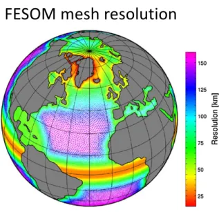
The surface computational grid used by FESOM is shown in Fig. 1. We use a spherical coordinate system with the poles over Greenland and the Antarctic continent to avoid convergence of meridians in the computational domain. The mesh has a nominal resolution of 150 km in the open ocean and is gradually refined to about 25 km in the northern North Atlantic and the tropics. We use iso- tropic grid refinement in the tropics since biases in tropi- cal regions are known to have a detrimental effect on the climate of the extratropics through atmospheric teleconnec- tions (see e.g., Rodwell and Jung 2008; Jung et al. 2010a), especially over the Northern Hemisphere. Grid refinement (meridional only) in the tropical belt is employed also in the regular-grid ocean components of other existing climate models (see e.g., Delworth et al. 2006; Gent et al. 2011).
The 3-dimensional mesh is formed by vertically extending the surface grid using 47 unevenly spaced z-levels and the ocean bottom is represented with shaved cells.
Although the latest version of FESOM (Wang et al.
2013) employs the K-Profile Parameterization (KPP) for vertical mixing (Large et al. 1994), we used the PP scheme by Pacanowski and Philander (1981) in this work. The rea- son is that by the time the coupled simulations were started, the performance of the KPP scheme in FESOM was not completely tested for long integrations in a global setting.
The mixing scheme may be changed to KPP in forthcom- ing simulations. The background vertical diffusion is set to 2×10⁻³m2s−1 for momentum and 10−5m2s−1 for potential temperature and salinity. The maximum value of vertical diffusivity and viscosity is limited to 0.01 m2s−1. We use the GM parameterization for the stirring due to Fig. 1 Grids correspond-
ing to (left) ECHAM6 at T63 (≈180 km) horizontal resolu- tion and (right) FESOM. The grid resolution for FESOM is indicated through color coding (in km). Dark green areas of the T63 grid correspond to areas where the land fraction exceeds 50 %; areas with a land fraction between 0 and 50 % are shown in light green
AWI-CM: ECHAM6-FESOM coupled model
Different models – same assimilation software
Lars Nerger et al. – Ensemble DA with PDAF
Coupled Models and Coupled Data Assimilation
Coupled models
• Several interconnected compartments, like
• Atmosphere and ocean
• Ocean physics and biogeochemistry (carbon, plankton, etc.)
Coupled data assimilation
• Assimilation into coupled models
• Weakly coupled: separate assimilation in the compartments
• Strongly coupled: joint assimilation of the compartments
➜ Use cross-covariances between fields in compartments
• Plus various “in between” possibilities …
€
759 ECHAM6–FESOM: model formulation and mean climate
1 3
2013) and uses total wavenumbers up to 63, which corre- sponds to about 1.85×1.85 degrees horizontal resolution;
the atmosphere comprises 47 levels and has its top at 0.01 hPa (approx. 80 km). ECHAM6 includes the land surface model JSBACH (Stevens et al. 2013) and a hydrological discharge model (Hagemann and Dümenil 1997).
Since with higher resolution “the simulated climate improves but changes are incremental” (Stevens et al.
2013), the T63L47 configuration appears to be a reason- able compromise between simulation quality and compu- tational efficiency. All standard settings are retained with the exception of the T63 land-sea mask, which is adjusted to allow for a better fit between the grids of the ocean and atmosphere components. The FESOM land-sea distribu- tion is regarded as ’truth’ and the (fractional) land-sea mask of ECHAM6 is adjusted accordingly. This adjustment is accomplished by a conservative remapping of the FESOM land-sea distribution to the T63 grid of ECHAM6 using an adapted routine that has primarily been used to map the land-sea mask of the MPIOM to ECHAM5 (H. Haak, per- sonal communication).
2.2 The Finite Element Sea Ice-Ocean Model (FESOM) The sea ice-ocean component in the coupled system is represented by FESOM, which allows one to simulate ocean and sea-ice dynamics on unstructured meshes with variable resolution. This makes it possible to refine areas of particular interest in a global setting and, for example, resolve narrow straits where needed. Additionally, FESOM allows for a smooth representation of coastlines and bottom topography. The basic principles of FESOM are described by Danilov et al. (2004), Wang et al. (2008), Timmermann et al. (2009) and Wang et al. (2013). FESOM has been validated in numerous studies with prescribed atmospheric forcing (see e.g., Sidorenko et al. 2011; Wang et al. 2012;
Danabasoglu et al. 2014). Although its numerics are fun- damentally different from that of regular-grid models,
previous model intercomparisons (see e.g., Sidorenko et al.
2011; Danabasoglu et al. 2014) show that FESOM is a competitive tool for studying the ocean general circulation.
The latest FESOM version, which is also used in this paper, is comprehensively described in Wang et al. (2013). In the following, we give a short model description here and men- tion those settings which are different in the coupled setup.
The surface computational grid used by FESOM is shown in Fig. 1. We use a spherical coordinate system with the poles over Greenland and the Antarctic continent to avoid convergence of meridians in the computational domain. The mesh has a nominal resolution of 150 km in the open ocean and is gradually refined to about 25 km in the northern North Atlantic and the tropics. We use iso- tropic grid refinement in the tropics since biases in tropi- cal regions are known to have a detrimental effect on the climate of the extratropics through atmospheric teleconnec- tions (see e.g., Rodwell and Jung 2008; Jung et al. 2010a), especially over the Northern Hemisphere. Grid refinement (meridional only) in the tropical belt is employed also in the regular-grid ocean components of other existing climate models (see e.g., Delworth et al. 2006; Gent et al. 2011).
The 3-dimensional mesh is formed by vertically extending the surface grid using 47 unevenly spaced z-levels and the ocean bottom is represented with shaved cells.
Although the latest version of FESOM (Wang et al.
2013) employs the K-Profile Parameterization (KPP) for vertical mixing (Large et al. 1994), we used the PP scheme by Pacanowski and Philander (1981) in this work. The rea- son is that by the time the coupled simulations were started, the performance of the KPP scheme in FESOM was not completely tested for long integrations in a global setting.
The mixing scheme may be changed to KPP in forthcom- ing simulations. The background vertical diffusion is set to 2×10⁻³m2s−1 for momentum and 10−5m2s−1 for potential temperature and salinity. The maximum value of vertical diffusivity and viscosity is limited to 0.01 m2s−1. We use the GM parameterization for the stirring due to Fig. 1 Grids correspond-
ing to (left) ECHAM6 at T63 (≈180 km) horizontal resolu- tion and (right) FESOM. The grid resolution for FESOM is indicated through color coding (in km). Dark green areas of the T63 grid correspond to areas where the land fraction exceeds 50 %; areas with a land fraction between 0 and 50 % are shown in light green
Atmosphere Ocean
coupling
Lars Nerger et al. – Ensemble DA with PDAF
Cpl. 1 Model Comp.
1 Task 1
2 compartment system – strongly coupled DA
Forecast Analysis Forecast
Model Comp.
1 Task 1
Model Comp.
2 Task 1 Cpl. 1
Model Comp.
1 Task 1
Cpl. 1 Model Comp.
1 Task 1 Model Comp.
1 Task 1
Model Comp.
2 Task 1 Cpl. 1
Model Comp.
1 Task 1 Filter
might be separate programs
Strongly coupled
Difficulties:
• Different assimilation frequency
• Different time scales
• Which fields are correlated?
• Do we have
(bi-)Gaussian
distributions?
Lars Nerger et al. – Ensemble DA with PDAF
Cpl. 2 Model Comp.
1 Task 2
2 compartment system – weakly coupled DA
Filter Comp. 1
Forecast Analysis Forecast
Model Comp.
1 Task 1
Model Comp.
2 Task 1 Cpl. 1
Model Comp.
2 Task 2
Cpl. 2 Model Comp.
1 Task 2 Model Comp.
1 Task 1
Model Comp.
2 Task 1 Cpl. 1
Model Comp.2
Task 2 Filter
Comp. 2
• Simpler setup than strongly coupled
• Different DA methods possible
• But:
Fields in different
compartments can be
inconsistent
Lars Nerger et al. – Ensemble DA with PDAF
Example 1
Assimilation into the coupled atmosphere-ocean model AWI-CM
(Qi Tang)
Project: ESM – Advanced Earth System Modeling Capacity
Lars Nerger et al. – Ensemble DA with PDAF
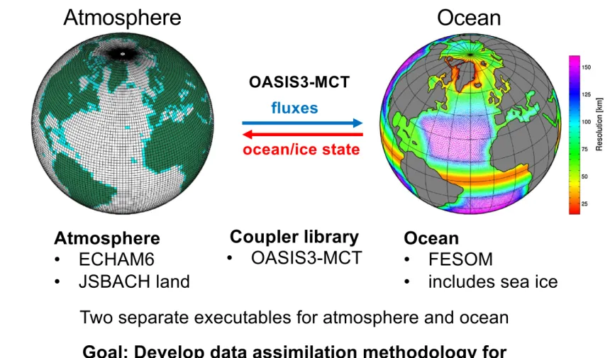
Assimilation into coupled model: AWI-CM
Atmosphere
• ECHAM6
• JSBACH land
759 ECHAM6–FESOM: model formulation and mean climate
1 3
2013) and uses total wavenumbers up to 63, which corre- sponds to about 1.85×1.85 degrees horizontal resolution;
the atmosphere comprises 47 levels and has its top at 0.01 hPa (approx. 80 km). ECHAM6 includes the land surface model JSBACH (Stevens et al. 2013) and a hydrological discharge model (Hagemann and Dümenil 1997).
Since with higher resolution “the simulated climate improves but changes are incremental” (Stevens et al.
2013), the T63L47 configuration appears to be a reason- able compromise between simulation quality and compu- tational efficiency. All standard settings are retained with the exception of the T63 land-sea mask, which is adjusted to allow for a better fit between the grids of the ocean and atmosphere components. The FESOM land-sea distribu- tion is regarded as ’truth’ and the (fractional) land-sea mask of ECHAM6 is adjusted accordingly. This adjustment is accomplished by a conservative remapping of the FESOM land-sea distribution to the T63 grid of ECHAM6 using an adapted routine that has primarily been used to map the land-sea mask of the MPIOM to ECHAM5 (H. Haak, per- sonal communication).
2.2 The Finite Element Sea Ice-Ocean Model (FESOM) The sea ice-ocean component in the coupled system is represented by FESOM, which allows one to simulate ocean and sea-ice dynamics on unstructured meshes with variable resolution. This makes it possible to refine areas of particular interest in a global setting and, for example, resolve narrow straits where needed. Additionally, FESOM allows for a smooth representation of coastlines and bottom topography. The basic principles of FESOM are described by Danilov et al. (2004), Wang et al. (2008), Timmermann et al. (2009) and Wang et al. (2013). FESOM has been validated in numerous studies with prescribed atmospheric forcing (see e.g., Sidorenko et al. 2011; Wang et al. 2012;
Danabasoglu et al. 2014). Although its numerics are fun- damentally different from that of regular-grid models,
previous model intercomparisons (see e.g., Sidorenko et al.
2011; Danabasoglu et al. 2014) show that FESOM is a competitive tool for studying the ocean general circulation.
The latest FESOM version, which is also used in this paper, is comprehensively described in Wang et al. (2013). In the following, we give a short model description here and men- tion those settings which are different in the coupled setup.
The surface computational grid used by FESOM is shown in Fig. 1. We use a spherical coordinate system with the poles over Greenland and the Antarctic continent to avoid convergence of meridians in the computational domain. The mesh has a nominal resolution of 150 km in the open ocean and is gradually refined to about 25 km in the northern North Atlantic and the tropics. We use iso- tropic grid refinement in the tropics since biases in tropi- cal regions are known to have a detrimental effect on the climate of the extratropics through atmospheric teleconnec- tions (see e.g., Rodwell and Jung 2008; Jung et al. 2010a), especially over the Northern Hemisphere. Grid refinement (meridional only) in the tropical belt is employed also in the regular-grid ocean components of other existing climate models (see e.g., Delworth et al. 2006; Gent et al. 2011).
The 3-dimensional mesh is formed by vertically extending the surface grid using 47 unevenly spaced z-levels and the ocean bottom is represented with shaved cells.
Although the latest version of FESOM (Wang et al.
2013) employs the K-Profile Parameterization (KPP) for vertical mixing (Large et al. 1994), we used the PP scheme by Pacanowski and Philander (1981) in this work. The rea- son is that by the time the coupled simulations were started, the performance of the KPP scheme in FESOM was not completely tested for long integrations in a global setting.
The mixing scheme may be changed to KPP in forthcom- ing simulations. The background vertical diffusion is set to 2×10⁻³m2s−1 for momentum and 10−5 m2s−1 for potential temperature and salinity. The maximum value of vertical diffusivity and viscosity is limited to 0.01 m2s−1. We use the GM parameterization for the stirring due to
Fig. 1 Grids correspond- ing to (left) ECHAM6 at T63 (≈180 km) horizontal resolu- tion and (right) FESOM. The grid resolution for FESOM is indicated through color coding (in km). Dark green areas of the T63 grid correspond to areas where the land fraction exceeds 50 %; areas with a land fraction between 0 and 50 % are shown in light green
Atmosphere Ocean
fluxes
ocean/ice state
759 ECHAM6–FESOM: model formulation and mean climate
1 3
2013) and uses total wavenumbers up to 63, which corre- sponds to about 1.85×1.85 degrees horizontal resolution;
the atmosphere comprises 47 levels and has its top at 0.01 hPa (approx. 80 km). ECHAM6 includes the land surface model JSBACH (Stevens et al. 2013) and a hydrological discharge model (Hagemann and Dümenil 1997).
Since with higher resolution “the simulated climate improves but changes are incremental” (Stevens et al.
2013), the T63L47 configuration appears to be a reason- able compromise between simulation quality and compu- tational efficiency. All standard settings are retained with the exception of the T63 land-sea mask, which is adjusted to allow for a better fit between the grids of the ocean and atmosphere components. The FESOM land-sea distribu- tion is regarded as ’truth’ and the (fractional) land-sea mask of ECHAM6 is adjusted accordingly. This adjustment is accomplished by a conservative remapping of the FESOM land-sea distribution to the T63 grid of ECHAM6 using an adapted routine that has primarily been used to map the land-sea mask of the MPIOM to ECHAM5 (H. Haak, per- sonal communication).
2.2 The Finite Element Sea Ice-Ocean Model (FESOM) The sea ice-ocean component in the coupled system is represented by FESOM, which allows one to simulate ocean and sea-ice dynamics on unstructured meshes with variable resolution. This makes it possible to refine areas of particular interest in a global setting and, for example, resolve narrow straits where needed. Additionally, FESOM allows for a smooth representation of coastlines and bottom topography. The basic principles of FESOM are described by Danilov et al. (2004), Wang et al. (2008), Timmermann et al. (2009) and Wang et al. (2013). FESOM has been validated in numerous studies with prescribed atmospheric forcing (see e.g., Sidorenko et al. 2011; Wang et al. 2012;
Danabasoglu et al. 2014). Although its numerics are fun- damentally different from that of regular-grid models,
previous model intercomparisons (see e.g., Sidorenko et al.
2011; Danabasoglu et al. 2014) show that FESOM is a competitive tool for studying the ocean general circulation.
The latest FESOM version, which is also used in this paper, is comprehensively described in Wang et al. (2013). In the following, we give a short model description here and men- tion those settings which are different in the coupled setup.
The surface computational grid used by FESOM is shown in Fig. 1. We use a spherical coordinate system with the poles over Greenland and the Antarctic continent to avoid convergence of meridians in the computational domain. The mesh has a nominal resolution of 150 km in the open ocean and is gradually refined to about 25 km in the northern North Atlantic and the tropics. We use iso- tropic grid refinement in the tropics since biases in tropi- cal regions are known to have a detrimental effect on the climate of the extratropics through atmospheric teleconnec- tions (see e.g., Rodwell and Jung 2008; Jung et al. 2010a), especially over the Northern Hemisphere. Grid refinement (meridional only) in the tropical belt is employed also in the regular-grid ocean components of other existing climate models (see e.g., Delworth et al. 2006; Gent et al. 2011).
The 3-dimensional mesh is formed by vertically extending the surface grid using 47 unevenly spaced z-levels and the ocean bottom is represented with shaved cells.
Although the latest version of FESOM (Wang et al.
2013) employs the K-Profile Parameterization (KPP) for vertical mixing (Large et al. 1994), we used the PP scheme by Pacanowski and Philander (1981) in this work. The rea- son is that by the time the coupled simulations were started, the performance of the KPP scheme in FESOM was not completely tested for long integrations in a global setting.
The mixing scheme may be changed to KPP in forthcom- ing simulations. The background vertical diffusion is set to 2×10⁻³m2s−1 for momentum and 10−5 m2s−1 for potential temperature and salinity. The maximum value of vertical diffusivity and viscosity is limited to 0.01 m2s−1. We use the GM parameterization for the stirring due to Fig. 1 Grids correspond-
ing to (left) ECHAM6 at T63 (≈180 km) horizontal resolu- tion and (right) FESOM. The grid resolution for FESOM is indicated through color coding (in km). Dark green areas of the T63 grid correspond to areas where the land fraction exceeds 50 %; areas with a land fraction between 0 and 50 % are shown in light green
OASIS3-MCT
Ocean
• FESOM
• includes sea ice Coupler library
• OASIS3-MCT
Two separate executables for atmosphere and ocean Goal: Develop data assimilation methodology for
cross-domain assimilation (“strongly-coupled”)
AWI-CM: Sidorenko et al., Clim Dyn 44 (2015) 757
Lars Nerger et al. – Ensemble DA with PDAF
Data Assimilation Experiments
• Observations
• Satellite SST
• Profiles temperature & salinity
• Updated: ocean state (SSH, T, S, u, v, w)
• Assimilation method: Ensemble Kalman Filter (LESTKF)
• Ensemble size: 46
• Simulation period: year 2016, daily assimilation update
• Run time: 5.5h, fully parallelized using 12,000 processor cores
Model setup
• Global model
• ECHAM6: T63L47
• FESOM: resolution 30-160km
Data assimilation experiments
759 ECHAM6–FESOM: model formulation and mean climate
1 3
2013) and uses total wavenumbers up to 63, which corre- sponds to about 1.85×1.85 degrees horizontal resolution;
the atmosphere comprises 47 levels and has its top at 0.01 hPa (approx. 80 km). ECHAM6 includes the land surface model JSBACH (Stevens et al. 2013) and a hydrological discharge model (Hagemann and Dümenil 1997).
Since with higher resolution “the simulated climate improves but changes are incremental” (Stevens et al.
2013), the T63L47 configuration appears to be a reason- able compromise between simulation quality and compu- tational efficiency. All standard settings are retained with the exception of the T63 land-sea mask, which is adjusted to allow for a better fit between the grids of the ocean and atmosphere components. The FESOM land-sea distribu- tion is regarded as ’truth’ and the (fractional) land-sea mask of ECHAM6 is adjusted accordingly. This adjustment is accomplished by a conservative remapping of the FESOM land-sea distribution to the T63 grid of ECHAM6 using an adapted routine that has primarily been used to map the land-sea mask of the MPIOM to ECHAM5 (H. Haak, per- sonal communication).
2.2 The Finite Element Sea Ice-Ocean Model (FESOM) The sea ice-ocean component in the coupled system is represented by FESOM, which allows one to simulate ocean and sea-ice dynamics on unstructured meshes with variable resolution. This makes it possible to refine areas of particular interest in a global setting and, for example, resolve narrow straits where needed. Additionally, FESOM allows for a smooth representation of coastlines and bottom topography. The basic principles of FESOM are described by Danilov et al. (2004), Wang et al. (2008), Timmermann et al. (2009) and Wang et al. (2013). FESOM has been validated in numerous studies with prescribed atmospheric forcing (see e.g., Sidorenko et al. 2011; Wang et al. 2012;
Danabasoglu et al. 2014). Although its numerics are fun- damentally different from that of regular-grid models,
previous model intercomparisons (see e.g., Sidorenko et al.
2011; Danabasoglu et al. 2014) show that FESOM is a competitive tool for studying the ocean general circulation.
The latest FESOM version, which is also used in this paper, is comprehensively described in Wang et al. (2013). In the following, we give a short model description here and men- tion those settings which are different in the coupled setup.
The surface computational grid used by FESOM is shown in Fig. 1. We use a spherical coordinate system with the poles over Greenland and the Antarctic continent to avoid convergence of meridians in the computational domain. The mesh has a nominal resolution of 150 km in the open ocean and is gradually refined to about 25 km in the northern North Atlantic and the tropics. We use iso- tropic grid refinement in the tropics since biases in tropi- cal regions are known to have a detrimental effect on the climate of the extratropics through atmospheric teleconnec- tions (see e.g., Rodwell and Jung 2008; Jung et al. 2010a), especially over the Northern Hemisphere. Grid refinement (meridional only) in the tropical belt is employed also in the regular-grid ocean components of other existing climate models (see e.g., Delworth et al. 2006; Gent et al. 2011).
The 3-dimensional mesh is formed by vertically extending the surface grid using 47 unevenly spaced z-levels and the ocean bottom is represented with shaved cells.
Although the latest version of FESOM (Wang et al.
2013) employs the K-Profile Parameterization (KPP) for vertical mixing (Large et al. 1994), we used the PP scheme by Pacanowski and Philander (1981) in this work. The rea- son is that by the time the coupled simulations were started, the performance of the KPP scheme in FESOM was not completely tested for long integrations in a global setting.
The mixing scheme may be changed to KPP in forthcom- ing simulations. The background vertical diffusion is set to 2×10⁻³ m2s−1 for momentum and 10−5m2s−1 for potential temperature and salinity. The maximum value of vertical diffusivity and viscosity is limited to 0.01 m2s−1. We use the GM parameterization for the stirring due to
Fig. 1 Grids correspond- ing to (left) ECHAM6 at T63 (≈180 km) horizontal resolu- tion and (right) FESOM. The grid resolution for FESOM is indicated through color coding (in km). Dark green areas of the T63 grid correspond to areas where the land fraction exceeds 50 %; areas with a land fraction between 0 and 50 % are shown in light green
FESOM mesh resolution
Lars Nerger et al. – Ensemble DA with PDAF
Offline coupling - Efficiency
Offline-coupling is simple to implement but can be very inefficent
Example:
Timing from atmosphere-ocean coupled model (AWI-CM)
with daily analysis step:
Model startup: 95 s Integrate 1 day: 28 s Model postprocessing: 14 s
Analysis step: 1 s
overhead
Restarting this model is ~3.5 times more expensive than integrating 1 day
➜ avoid this for data assimilation
Lars Nerger et al. – Ensemble DA with PDAF
0 10 20 30 40 50
ensemble size 0
5 10 15 20 25 30 35 40
time [s]
Execution times per model day
forecast couple forecast-couple analysis prepoststep
Execution times (weakly-coupled, DA only into ocean)
MPI-tasks
• ECHAM: 72
• FESOM: 192
• Increasing integration time with growing ensemble size (11%; more parallel
communication; worse placement)
• some variability in integration time over ensemble tasks
12,144 processor
cores
Important factors for good performance
• Need optimal distribution of programs over compute nodes/racks (here set up as ocean/atmosphere pairs)
• Avoid conflicts in IO (Best performance when each AWI- CM task runs in separate directory)
528 processor
cores
Lars Nerger et al. – Ensemble DA with PDAF
Assimilate sea surface temperature (SST)
• Satellite sea surface temperature (level 3, EU Copernicus)
• Daily data
• Data gaps due to clouds
• Observation error: 0.8
oC
• Localization radius: 1000 km
SST on Jan 1 st , 2016
SST difference: observations-model
Large initial SST deviation due to using a coupled model: up to 10
oC DA with such a coupled model is unstable!
omit SST observations where
|SST
obs- SST
ens_mean| > 1.6
oC
(30% initially, <5% later)
Lars Nerger et al. – Ensemble DA with PDAF
SST assimilation: Effect on the ocean
SST difference (obs-model): strong decrease of deviation
Free run 4/30/2016 Assimilation
Day 120
Subsurface temperature difference (obs-model); all the model layers at profile locations
4/30/2016 Day 120
Free run Assimilation
Lars Nerger et al. – Ensemble DA with PDAF
Assimilate subsurface observations: Profiles
• Temperature and Salinity
• EN4 data from UK MetOffice
• Daily data
• Subsurface down to 5000m
• About 1000 profiles per day
• Observation errors
– Temperature profiles: 0.8
oC – Salinity profiles: 0.5 psu
• Localization radius: 1000 km
Profile locations on Jan 1
st, 2016
Lars Nerger et al. – Ensemble DA with PDAF
SST assimilation: Effect on the ocean
SST difference (obs-model)
Free run 4/30/2016 Assimilation
Day 120
Subsurface temperature difference (obs-model); all the model layers at profile locations
4/30/2016 Day 120
Free run Assimilation
larger deviations than for SST assimilation
smaller deviations
than for SST
assimilation
Lars Nerger et al. – Ensemble DA with PDAF
Assimilation effect: RMS errors
0,00 0,50 1,00 1,50 2,00 2,50 3,00
RMSE(SST) RMSE(proT) RMSE(proS) Free_run DA_SST DA_proTS DA_all
Overall lowest errors with combined assimilation
• But partly a compromise
Lars Nerger et al. – Ensemble DA with PDAF
Mean increments
Surface temperature
Mean increments (analysis – forecast) for days 61-366 (after spinup)
➜ non-zero values indicate regions with possible biases
Temperature at
100m depth
Lars Nerger et al. – Ensemble DA with PDAF
Assimilation Effect on the Atmosphere
Temperature at 2m
Difference between assimilation runs and the free run
Sea surface temperature
Atmosphere reacts quickly on the changed ocean state
Does it make the atmosphere more realistic?
Lars Nerger et al. – Ensemble DA with PDAF
2-meter temperature
Free run Assimilation
10 meter zonal wind velocity
Free run Assimilation
Effect on Atmospheric State (annual mean)
Te m p e ra tu re (
oC ) / Ve lo ci ty (m /s )
Next step: strongly coupled assimilation
assimilate ocean SST into the atmosphere technically rather simple – in practice?
Relevant is
ocean surface
Lars Nerger et al. – Ensemble DA with PDAF
Strongly coupled: Parallelization of analysis step
We need innovation: d = Hx - y
Observation operator links different compartments
1. Compute part of d on process
‘owning’ the observation
2. Communicate d to processes for which observation is within
localization radius
State vector X
At m o sp h e re Oce a n
Proc. 0
Proc. k
Hx
apply H
Comm.
distribute d
Lars Nerger et al. – Ensemble DA with PDAF
Example 2
Weakly- and Strongly Coupled Assimilation to Constrain Biogeochemistry with Temperature Data
(MERAMO – Mike Goodliff)
Cooperation with German Hydrographic Agency (BSH)
(Ina Lorkowski, Xin Li, Anja Lindenthal, Thoger Brüning)
Lars Nerger et al. – Ensemble DA with PDAF
Coastal Model Domain
5 km
900 m
Grid with higher resolution in German coastal region
HBM (Hiromb-BOOS Model) – operationally used at German
Federal Maritime and Hydrographic Agency (BSH)
Lars Nerger et al. – Ensemble DA with PDAF
Biogeochemical model: ERGOM
Atmosphere
Ocean
Sediment
PO
43-N
2O
2Cyanobacteria
Diatoms Flagellates
Detritus N
Micro- zooplankton
Si NO
3-NH
4+O
2Meso- zooplankton Detritus Si
N
2Phytoplankton Zooplankton
Nutrients
Lars Nerger et al. – Ensemble DA with PDAF
Observations – Sea Surface Temperature (SST)
• 12-hour composites on both model grids
• Vastly varying data coverage (due to clouds)
• Effect on biogeochemistry?
NOAA/AVHRR Satellite data
10 April 2012 25 May 2012
Lars Nerger et al. – Ensemble DA with PDAF
Comparison with assimilated SST data (4-12/2012)
l
RMS deviation from SST observations up to ~0.4
oC Coarse grid:
l
Increasing error-reductions compared to free ensemble run
coarse grid Temperature RMSD
Fine grid:
l
much stronger variability
l
Forecast errors sometimes reach errors of free ensemble run
fine grid
Free Forec. Ana.
Coarse 0.95 0.68 0.63
Fine 0.83 0.70 0.63
RMS errors (deg. C)
Lars Nerger et al. – Ensemble DA with PDAF
Influence of Assimilation on Surface Temperature
Change of Temperature (Oct. 2017) Change of Oxygen concentration
2 ways of influence:
• Indirect - weakly-coupled assimilation
model dynamics react on change in physics
• Direct – strongly-coupled assimilation
use cross-covariances between surface temperature and biogeochemistry
Lars Nerger et al. – Ensemble DA with PDAF
Weakly & strongly coupled effect on biogeochemical model
l
Changes up to 8% (slight error reductions)
l
Larger in Baltic than North Sea
Free run
Oxygen mean for May 2012 (as mmol O / m
3)
Free run Assimilation WEAK
Strongly coupled
l
slightly larger changes
l