Coupled Data Assimilation for Ocean-Biogeochemical Models Lars Nerger, Himansu Pradhan, Michael Goodliff

(1)

Coupled Data Assimilation

for Ocean-Biogeochemical Models

Lars Nerger, Himansu Pradhan, Michael Goodliff

Alfred Wegener Institute

Helmholtz Center for Polar and Marine Research Bremerhaven, Germany

ISDA 2019, Kobe, Japan, January 21 – 24, 2019

AWI

(2)

Lars Nerger et al. – Coupled DA for Ocean Biogeochemical Models

Coupled Ocean-Biogeochemical Models

Physics

Ocean Circulation Model

Regulated Ecosystem Model – Version 2

REcoM2

759 ECHAM6–FESOM: model formulation and mean climate

1 3

2013) and uses total wavenumbers up to 63, which corre- sponds to about 1.85×1.85 degrees horizontal resolution;

the atmosphere comprises 47 levels and has its top at 0.01 hPa (approx. 80 km). ECHAM6 includes the land surface model JSBACH (Stevens et al. 2013) and a hydrological discharge model (Hagemann and Dümenil 1997).

Since with higher resolution “the simulated climate improves but changes are incremental” (Stevens et al.

2013), the T63L47 configuration appears to be a reason- able compromise between simulation quality and computational efficiency. All standard settings are retained with the exception of the T63 land-sea mask, which is adjusted to allow for a better fit between the grids of the ocean and atmosphere components. The FESOM land-sea distribution is regarded as ’truth’ and the (fractional) land-sea mask of ECHAM6 is adjusted accordingly. This adjustment is accomplished by a conservative remapping of the FESOM land-sea distribution to the T63 grid of ECHAM6 using an adapted routine that has primarily been used to map the land-sea mask of the MPIOM to ECHAM5 (H. Haak, per- sonal communication).

2.2 The Finite Element Sea Ice-Ocean Model (FESOM) The sea ice-ocean component in the coupled system is represented by FESOM, which allows one to simulate ocean and sea-ice dynamics on unstructured meshes with variable resolution. This makes it possible to refine areas of particular interest in a global setting and, for example, resolve narrow straits where needed. Additionally, FESOM allows for a smooth representation of coastlines and bottom topography. The basic principles of FESOM are described by Danilov et al. (2004), Wang et al. (2008), Timmermann et al. (2009) and Wang et al. (2013). FESOM has been validated in numerous studies with prescribed atmospheric forcing (see e.g., Sidorenko et al. 2011; Wang et al. 2012;

Danabasoglu et al. 2014). Although its numerics are fun- damentally different from that of regular-grid models,

previous model intercomparisons (see e.g., Sidorenko et al.

2011; Danabasoglu et al. 2014) show that FESOM is a competitive tool for studying the ocean general circulation.

The latest FESOM version, which is also used in this paper, is comprehensively described in Wang et al. (2013). In the following, we give a short model description here and men- tion those settings which are different in the coupled setup.

The surface computational grid used by FESOM is shown in Fig. 1. We use a spherical coordinate system with the poles over Greenland and the Antarctic continent to avoid convergence of meridians in the computational domain. The mesh has a nominal resolution of 150 km in the open ocean and is gradually refined to about 25 km in the northern North Atlantic and the tropics. We use iso- tropic grid refinement in the tropics since biases in tropical regions are known to have a detrimental effect on the climate of the extratropics through atmospheric teleconnec- tions (see e.g., Rodwell and Jung 2008; Jung et al. 2010a), especially over the Northern Hemisphere. Grid refinement (meridional only) in the tropical belt is employed also in the regular-grid ocean components of other existing climate models (see e.g., Delworth et al. 2006; Gent et al. 2011).

The 3-dimensional mesh is formed by vertically extending the surface grid using 47 unevenly spaced z-levels and the ocean bottom is represented with shaved cells.

Although the latest version of FESOM (Wang et al.

2013) employs the K-Profile Parameterization (KPP) for vertical mixing (Large et al. 1994), we used the PP scheme by Pacanowski and Philander (1981) in this work. The reason is that by the time the coupled simulations were started, the performance of the KPP scheme in FESOM was not completely tested for long integrations in a global setting.

The mixing scheme may be changed to KPP in forthcom- ing simulations. The background vertical diffusion is set to 2×10⁻³m²s⁻¹ for momentum and 10⁻⁵m²s⁻¹ for potential temperature and salinity. The maximum value of vertical diffusivity and viscosity is limited to 0.01 m²s⁻¹. We use the GM parameterization for the stirring due to Fig. 1 Grids correspond-

ing to (left) ECHAM6 at T63 (≈180 km) horizontal resolution and (right) FESOM. The grid resolution for FESOM is indicated through color coding (in km). Dark green areas of the T63 grid correspond to areas where the land fraction exceeds 50 %; areas with a land fraction between 0 and 50 % are shown in light green

Ecosystem

Biogeochemical Model, …

Finite-Element Sea Ice Ocean Model

FESOM

coupling

velocities

Temperature

(3)

Biogeochemical Process Models

Example: REcoM-2

Regulated Ecosystem Model – Version 2 (Hauck et al., 2013 )

Wide variations of the model formulation

(4)

Satellite Ocean Color Observations

Natural Color 3/16/2004

Picture source:

Suomi-NPP/VIIRS, December 10, 2018 NASA (oceancolor.gsfc.nasa.gov)

This is not a photograph!

spectral bands in ESA OC-CCI data

Spectral data at 5-8 wavelengths in visible part of spectrum

• Satellite data is water leaving radiance or surface reflectance

➜ Data products are derived

from this

(5)

Satellite Chlorophyll Data (the most common product)

Natural Color 3/16/2004 Chlorophyll Concentrations

Figure: NASA Visible Earth , Image: SeaWiFS Project, NASA/GSFC & Orbimage

Chlorophyll computed as

4

^th

order polynomial of reflectance at two wavelengths:

or combined with linear three-wavelength dependence log

₁₀

(CHL

_a

) = a

₀

+

X

4

i=1

a

_i

✓

log

₁₀

✓ R(

_blue

) R(

_green

)

◆◆

i

<latexit sha1_base64="qnJs0B1X5/hxhzawdCAyXmmdvxQ=">AAACYXicbZFNa9wwEIZlN22STZM66TEXkSWwSyHYJdBeAqG55NBDWrJJYL0xY+3YKyLLRhqHLMZ/srdeeukfqXbXhXwNCL16ZoaRXqWVkpbC8Lfnv1l7+259Y7O39X5750Owu3dly9oIHIlSleYmBYtKahyRJIU3lUEoUoXX6d3ZIn99j8bKUl/SvMJJAbmWmRRADiXBgyrzpInCdnB2/j2BIT/hkIT8E49tXSSNPIna22OHZKwwo8H/6tUpzgyI5ucgVm7gFJImVTW2w/Yxyg2idiw2Mp/RsNtuZRL0w6NwGfyliDrRZ11cJMGveFqKukBNQoG14yisaNKAISkUtr24tliBuIMcx05qKNBOmqVDLT90ZMqz0riliS/p444GCmvnReoqC6CZfZ5bwNdy45qyr5NG6qom1GI1KKsVp5Iv7OZTaVCQmjsBwkh3Vy5m4Gwj9yk9Z0L0/MkvxdXno8jpH8f902+dHRtsnx2wAYvYF3bKztkFGzHB/nhr3ra34/31N/3A31uV+l7X85E9CX//H7XntUo=</latexit><latexit sha1_base64="qnJs0B1X5/hxhzawdCAyXmmdvxQ=">AAACYXicbZFNa9wwEIZlN22STZM66TEXkSWwSyHYJdBeAqG55NBDWrJJYL0xY+3YKyLLRhqHLMZ/srdeeukfqXbXhXwNCL16ZoaRXqWVkpbC8Lfnv1l7+259Y7O39X5750Owu3dly9oIHIlSleYmBYtKahyRJIU3lUEoUoXX6d3ZIn99j8bKUl/SvMJJAbmWmRRADiXBgyrzpInCdnB2/j2BIT/hkIT8E49tXSSNPIna22OHZKwwo8H/6tUpzgyI5ucgVm7gFJImVTW2w/Yxyg2idiw2Mp/RsNtuZRL0w6NwGfyliDrRZ11cJMGveFqKukBNQoG14yisaNKAISkUtr24tliBuIMcx05qKNBOmqVDLT90ZMqz0riliS/p444GCmvnReoqC6CZfZ5bwNdy45qyr5NG6qom1GI1KKsVp5Iv7OZTaVCQmjsBwkh3Vy5m4Gwj9yk9Z0L0/MkvxdXno8jpH8f902+dHRtsnx2wAYvYF3bKztkFGzHB/nhr3ra34/31N/3A31uV+l7X85E9CX//H7XntUo=</latexit><latexit sha1_base64="qnJs0B1X5/hxhzawdCAyXmmdvxQ=">AAACYXicbZFNa9wwEIZlN22STZM66TEXkSWwSyHYJdBeAqG55NBDWrJJYL0xY+3YKyLLRhqHLMZ/srdeeukfqXbXhXwNCL16ZoaRXqWVkpbC8Lfnv1l7+259Y7O39X5750Owu3dly9oIHIlSleYmBYtKahyRJIU3lUEoUoXX6d3ZIn99j8bKUl/SvMJJAbmWmRRADiXBgyrzpInCdnB2/j2BIT/hkIT8E49tXSSNPIna22OHZKwwo8H/6tUpzgyI5ucgVm7gFJImVTW2w/Yxyg2idiw2Mp/RsNtuZRL0w6NwGfyliDrRZ11cJMGveFqKukBNQoG14yisaNKAISkUtr24tliBuIMcx05qKNBOmqVDLT90ZMqz0riliS/p444GCmvnReoqC6CZfZ5bwNdy45qyr5NG6qom1GI1KKsVp5Iv7OZTaVCQmjsBwkh3Vy5m4Gwj9yk9Z0L0/MkvxdXno8jpH8f902+dHRtsnx2wAYvYF3bKztkFGzHB/nhr3ra34/31N/3A31uV+l7X85E9CX//H7XntUo=</latexit><latexit sha1_base64="qnJs0B1X5/hxhzawdCAyXmmdvxQ=">AAACYXicbZFNa9wwEIZlN22STZM66TEXkSWwSyHYJdBeAqG55NBDWrJJYL0xY+3YKyLLRhqHLMZ/srdeeukfqXbXhXwNCL16ZoaRXqWVkpbC8Lfnv1l7+259Y7O39X5750Owu3dly9oIHIlSleYmBYtKahyRJIU3lUEoUoXX6d3ZIn99j8bKUl/SvMJJAbmWmRRADiXBgyrzpInCdnB2/j2BIT/hkIT8E49tXSSNPIna22OHZKwwo8H/6tUpzgyI5ucgVm7gFJImVTW2w/Yxyg2idiw2Mp/RsNtuZRL0w6NwGfyliDrRZ11cJMGveFqKukBNQoG14yisaNKAISkUtr24tliBuIMcx05qKNBOmqVDLT90ZMqz0riliS/p444GCmvnReoqC6CZfZ5bwNdy45qyr5NG6qom1GI1KKsVp5Iv7OZTaVCQmjsBwkh3Vy5m4Gwj9yk9Z0L0/MkvxdXno8jpH8f902+dHRtsnx2wAYvYF3bKztkFGzHB/nhr3ra34/31N/3A31uV+l7X85E9CX//H7XntUo=</latexit>

(this is empirical! – derived from statistical analysis)

(6)

Daily gridded SeaWiFS chlorophyll data Ø gaps: satellite track, clouds, polar nights Ø 30% to 50% data coverage

Ø irregular data availability

Example: Chlorophyll-a (SeaWiFS)

mg/m³

Nerger, L., and W.W. Gregg. J. Marine Systems68 (2007) 237

(7)

Model

• Skill

• Complexity Observations

• Data gaps

• Data error level

• Empiric algorithms Assimilation

• Approx. log-normal

• Diurnal variability

• Representation errors

Data Assimilation Issues

Much higher error than in physics Only fraction of fields observed

Fields are less constrained 15 - 30%

representation error

Need to transform concentrations representation error

Unknown, but expected to be high

(8)

Example 1

Assimilation of total chlorophyll

to constrain 2 phytoplankton groups

(9)

Example: Global Chlorophyll Assimilation

Global configuration

80

^o

N - 80

^o

S, 30 layers Resolution:

lon : 2 deg

lat : 2 deg in North

up to 0.38 deg in South

MITgcm

General ocean circulation model of MIT (Marshall et al., 1997).

REcoM-2

Regulated Ecosystem Model – Version 2

(Hauck et al., 2013 )

Assimilate with PDAF (http://pdaf.awi.de)

(10)

Assimilation:

• Assimilate satellite total chlorophyll (ESA Ocean color - climate change initiative):

Chl

_TOT

= Chl

_DIA

+ Chl

_PHY

• Handle logarithmic concentrations log(Chl

_TOT

), log(Chl

_DIA

), log(Chl

_PHY

)

• Multivariate update through, e.g.

Cov(log(Chl

_TOT

), log(Chl

_DIA

))

• How are both phytoplankton groups influenced?

• Validate with satellite and in situ data

Assimilated:

Total chlorophyll from ESA OC-CCI

Assimilation of Total Chlorophyll

logarithmic observation errors

Total chlorophyll (5 day composite) ^mg/m³

(11)

Verification: Phytoplankton group data SynSenPFT (Losa et al. 2018)

mg/m³

Small phytoplankton

Diatoms ^mg/m³

Assimilated:

Total chlorophyll from ESA OC-CCI

Assimilation of Total Chlorophyll

logarithmic observation errors

Total chlorophyll (5 day composite) ^mg/m³

(12)

Effect on Chlorophyll in Phytoplankton Groups

• Assimilation improves groups individually through cross-

covariances

• Stronger error-reductions for Diatoms

• In situ data comparison:

(bias and correlation also improved)

logarithmic RMS errors (southern regions)

Diatoms Small phytoplankton

Pradhan et al., J. Geophy. Res. Oceans, in press, doi:10.1029/2018JC014329

Current work

• Asses impact of assimilating chlorophyll group data

(much lower errors for diatoms)

RMSe Free Assim.

Diatoms 1.3 0.91

Small Phyto. 0.53 0.45

(13)

Ensemble-estimated Cross-correlations

• Significantly different correlations for small phytoplankton and diatoms

• Negative correlations exist (despite Chl

_TOT

= Chl

_DIA

+ Chl

_PHY

) Cross correlations between total and group chlorophyll

Pradhan et al., J. Geophy. Res. Oceans, in press, doi:10.1029/2018JC014329

(14)

Example 2

Weakly- and Strongly Coupled Assimilation

Constrain Biogeochemistry with Temperature Data

(15)

Lars Nerger et al. – Coupled DA for Ocean Biogeochemical Models 759

ECHAM6–FESOM: model formulation and mean climate

1 3

2013) and uses total wavenumbers up to 63, which corre- sponds to about 1.85 ×1.85 degrees horizontal resolution;

the atmosphere comprises 47 levels and has its top at 0.01 hPa (approx. 80 km). ECHAM6 includes the land surface model JSBACH (Stevens et al. 2013) and a hydrological discharge model (Hagemann and Dümenil 1997).

Since with higher resolution “the simulated climate improves but changes are incremental” (Stevens et al.

2013), the T63L47 configuration appears to be a reason- able compromise between simulation quality and computational efficiency. All standard settings are retained with the exception of the T63 land-sea mask, which is adjusted to allow for a better fit between the grids of the ocean and atmosphere components. The FESOM land-sea distribution is regarded as ’truth’ and the (fractional) land-sea mask of ECHAM6 is adjusted accordingly. This adjustment is accomplished by a conservative remapping of the FESOM land-sea distribution to the T63 grid of ECHAM6 using an adapted routine that has primarily been used to map the land-sea mask of the MPIOM to ECHAM5 (H. Haak, per- sonal communication).

2.2 The Finite Element Sea Ice-Ocean Model (FESOM) The sea ice-ocean component in the coupled system is represented by FESOM, which allows one to simulate ocean and sea-ice dynamics on unstructured meshes with variable resolution. This makes it possible to refine areas of particular interest in a global setting and, for example, resolve narrow straits where needed. Additionally, FESOM allows for a smooth representation of coastlines and bottom topography. The basic principles of FESOM are described by Danilov et al. (2004), Wang et al. (2008), Timmermann et al. (2009) and Wang et al. (2013). FESOM has been validated in numerous studies with prescribed atmospheric forcing (see e.g., Sidorenko et al. 2011; Wang et al. 2012;

Danabasoglu et al. 2014). Although its numerics are fun- damentally different from that of regular-grid models,

previous model intercomparisons (see e.g., Sidorenko et al.

2011; Danabasoglu et al. 2014) show that FESOM is a competitive tool for studying the ocean general circulation.

The latest FESOM version, which is also used in this paper, is comprehensively described in Wang et al. (2013). In the following, we give a short model description here and men- tion those settings which are different in the coupled setup.

The surface computational grid used by FESOM is shown in Fig. 1. We use a spherical coordinate system with the poles over Greenland and the Antarctic continent to avoid convergence of meridians in the computational domain. The mesh has a nominal resolution of 150 km in the open ocean and is gradually refined to about 25 km in the northern North Atlantic and the tropics. We use iso- tropic grid refinement in the tropics since biases in tropical regions are known to have a detrimental effect on the climate of the extratropics through atmospheric teleconnec- tions (see e.g., Rodwell and Jung 2008; Jung et al. 2010a), especially over the Northern Hemisphere. Grid refinement (meridional only) in the tropical belt is employed also in the regular-grid ocean components of other existing climate models (see e.g., Delworth et al. 2006; Gent et al. 2011).

The 3-dimensional mesh is formed by vertically extending the surface grid using 47 unevenly spaced z-levels and the ocean bottom is represented with shaved cells.

Although the latest version of FESOM (Wang et al.

2013) employs the K-Profile Parameterization (KPP) for vertical mixing (Large et al. 1994), we used the PP scheme by Pacanowski and Philander (1981) in this work. The reason is that by the time the coupled simulations were started, the performance of the KPP scheme in FESOM was not completely tested for long integrations in a global setting.

The mixing scheme may be changed to KPP in forthcom- ing simulations. The background vertical diffusion is set to 2×10⁻³ m²s⁻¹ for momentum and 10⁻⁵ m²s⁻¹ for potential temperature and salinity. The maximum value of vertical diffusivity and viscosity is limited to 0.01 m²s⁻¹. We use the GM parameterization for the stirring due to

Fig. 1 Grids correspond- ing to (left) ECHAM6 at T63 (≈180 km) horizontal resolution and (right) FESOM. The grid resolution for FESOM is indicated through color coding (in km). Dark green areas of the T63 grid correspond to areas where the land fraction exceeds 50 %; areas with a land fraction between 0 and 50 % are shown in light green

Example: weakly- and strongly coupled assimilation

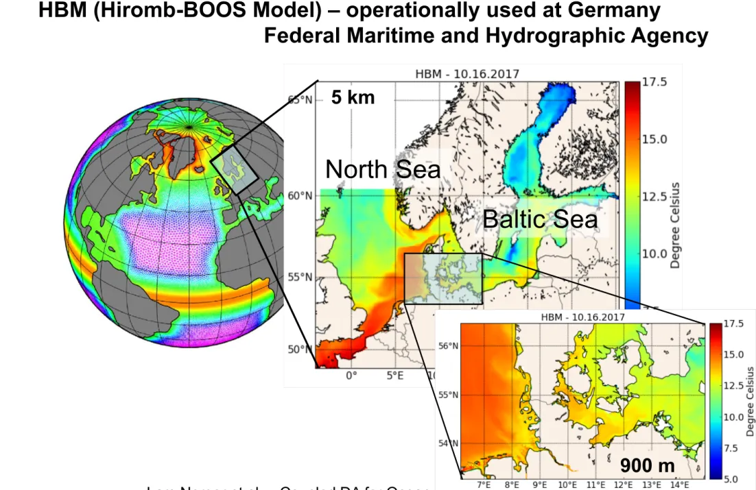
HBM (Hiromb-BOOS Model) – operationally used at Germany

Federal Maritime and Hydrographic Agency

5 km

Baltic Sea North Sea

900 m

(16)

Biogeochemical model: ERGOM

Atmosphere

Ocean

Sediment

PO

₄^3-

N

₂

O

₂

Cyanobacteria

Diatoms Flagellates

Detritus N

Micro- zooplankton

Si NO

₃^-

NH

₄⁺

O

₂

Meso- zooplankton Detritus Si

N

₂

Phytoplankton Zooplankton

Nutrients

(17)

Observations – Sea Surface Temperature (SST)

• 12-hour composites

• Vastly varying data coverage (due to clouds)

• Effect on biogeochemistry?

• Assimilation using assimilation framework PDAF

NOAA/AVHRR Satellite data

10 April 2012 25 May 2012

(18)

Weakly & strongly coupled effect on biogeochemistry

l

Changes up to 8% (slight error reductions)

l

Larger in Baltic than North Sea

Free run

Oxygen mean for May 2012 (as mmol O / m

³

)

Free run Assimilation WEAK Free – Assimilation WEAK

(19)

Assimilation STRONG

Weakly & strongly coupled effect on biogeochemistry

Free run

Oxygen mean for May 2012 (as mmol O / m

³

)

Free run Assimilation WEAK

Strongly coupled

l

slightly larger changes

l

Strongly coupled DA further improves

oxygen

l

Used actual (linear) concentrations

Free – Assimilation WEAK

Free – Assimilation STRONG

(20)

Using Logarithmic Concentrations

Free run

Oxygen mean for May 2012 (as mmol O / m

³

)

Free run Assimilation STRONG-lin Assimilation STRONG-log

STRONG-log vertical localization 10m

Use logarithmic concentrations in analysis step

➜ Unrealistic concentrations

• Much too high in deeper ocean regions

• Caused by unrealistic cross-covariances between SST & sub-surface oxygen

Vertical localization

➜ Helps in most regions (but not all)

➜ Is log-normal assumption correct?

(21)