An extended variational atmospheric chemistry data assimilation system for
combined space and air borne trace gas retrievals
I n a u g u r a l – D i s s e r t a t i o n zur
Erlangung des Doktorgrades
der Mathematisch–Naturwissenschaftlichen Fakult¨at der Universit¨at zu K¨oln
vorgelegt von
Ketevan Kasradze
aus Tbilisi
K¨oln 2016
Berichterstatter: PD Dr. H. Elbern Prof. Dr. A. Wahner
Tag der m¨undlichen Pr¨ufung: 28.06.2016
Abstract
A four-dimensional variational data assimilation system for stratospheric trace gas observations has been extended and evaluated to draw full advantage from stratospheric remote sounding data and upper troposphere lower strato- sphere (UTLS) in-situ aircraft measurements. The UTLS is the transition layer between the stratosphere and the troposphere and is marked by strong spatial and temporal variability of dynamic structures and distribution of trace gases.
Aircraft measurements, highly resolving the UTLS filamental structures, are of most interest for local studies. Although, the satellite instruments are deliver- ing an unprecedented wealth of observations of a number of stratospheric trace gases with global coverage, they are scattered and have a limited resolution in space or time. Combining these measurements and applying advanced data assimilation techniques to compare benefits from satellite and air borne data, and to analyse the chemical composition of the tropopause and lower strato- sphere, was the issue of this work. For this purpose, a model grid refinement and full revision of the chemical mechanism were performed. The resolution of the horizontal grid points was increased from about 240 km to 150 km, resulting in 23 042 grid points per model level. The vertical resolution was increased with twelve additional layers, especially in the UTLS region. Hence, the vertical separation between grid levels is now less than 1 km below 22 km altitude. The chemistry module was extended and revised to better represent chemical processes in the UTLS region. All reaction rates were updated ac- cording to the recommendations of the NASA’s Jet Propulsion Laboratory. In total, a number of 197 photolysis, gas phase, and heterogeneous reactions of 51 stratospheric trace gases is considered by the chemistry module now. The meteorological fields are computed online by the global forecast model GME of German Weather Service. A comprehensive set of case studies has been con- ducted in order to test and evaluate the extended system. Retrievals of various stratospheric trace gases derived from measurements of the Earth Observing System Microwave Limb Sounder, as well as retrievals of aircraft measurements have been assimilated. The analyses show a perfect performance with respect to the assimilated ozone observations. For assimilation of water observations in UTLS additional preconditioning issue is desirable. Comparison with inde- pendent observations from satellite instruments and radiosondes demonstrates a very good performance of the extended assimilation system.
Kurzzusammenfassung
Ein System zur Assimilation stratosph¨arischer Spurengasmessungen basierend auf der vierdimensionalen variationellen Methode wurde erweitert und vali- diert. Dies wurde durchgef¨uhrt um die Vorteile stratosph¨arischer Fernerkun- dungsdaten und in-situ Flugzeugmessungen in der oberen Troposph¨are und der unteren Stratosph¨are (UTLS) zu vereinen. Die UTLS ist die ¨Ubergangsschicht zwischen der Stratosph¨are und der Troposph¨are und wird durch starke r¨aum- liche und zeitliche Variabilit¨at der dynamischen Strukturen gekennzeichnet.
Flugzeugmessungen k¨onnen die filament¨are Strukturen in der UTLS aufl¨osen und sind f¨ur lokale Studien von besonderem Interesse. Obwohl Satelliteninstru- mente eine große Anzahl an Beobachtungen von Spurengasen in der gesamten Stratosph¨are liefern, haben sie nur begrenzte Aufl¨osung in Raum oder Zeit.
Dieser Beobachtungen zu kombinieren und erweiterte Datenassimilationstech- niken anzuwenden, um die chemische Zusammensetzung der Tropopause und der unteren Stratosph¨are zu analysieren, ist das Hauptziel dieser Arbeit. Zu diesem Zweck wurde das Modellgitter verfeinert und der chemische Mechanis- mus vollst¨andig ¨uberarbeitet. Die horizontale Aufl¨osung wurde von etwa 240 km auf 150 km erh¨oht und resultiert in 23 042 Gitterpunkten pro Modellebene.
Die vertikale Aufl¨osung wurde um zus¨atzliche zw¨olf Schichten erh¨oht, insbe- sondere in der UTLS Region. Die vertikale Ausdehnung einzelner Schichten ist dadurch kleiner als 1 km unterhalb von 22 km H¨ohe. Das neue Chemiemodul ber¨ucksichtigt 197 Photolyse-, Gasphasen- und heterogene Reaktionen zwi- schen 51 stratosph¨arischen Spurengasen. Die meteorologischen Felder werden mit Hilfe des globalen Wettervorhersagemodells GME des Deutschen Wetter- dienstes direkt erzeugt. Die Leistung des neu erweiterten vierdimensionalen variationellen Datenassimilationsystems wurde mit Fallstudien validiert. Da- zu wurden Spurengasprofile, abgeleitet aus Messungen des “Earth Observing System Microwave Limb Sounder” sowie Beobachtungen von Flugzeugmessun- gen wurden assimiliert. Die Analysen zeigen eine perfekte ¨Ubereinstimmung mit assimilierten Ozonbeobachtungen. F¨ur die assimilation von Wasserbeob- achtungen in der UTLS eine zus¨atzliche Pr¨akonditionierung vorzuziehen. Der Vergleich mit unabh¨angigen Beobachtungen von Satelliteninstrumenten und Radiosonden demonstriert eine sehr gute Leistung des erweiterten Assimilati- onssystems.
Contents
1 Introduction 1
2 Data assimilation 5
2.1 Bayes’ theorem . . . . 5
2.2 Maximum likelihood and minimum variance . . . . 6
2.3 Four-dimensional variational data assimilation . . . . 7
2.3.1 Adjoint model technique . . . . 9
3 The SACADA assimilation system 11 3.1 The SACADA model . . . 12
3.2 Chemistry transport module . . . 13
3.3 The adjoint model . . . 15
3.4 Meteorological module, grid configuration and parallelization . . 16
4 Background error covariance modeling 21 4.1 Incremental formulation of the cost function . . . 22
4.2 Correlation modelling with diffusion approach . . . 23
4.3 Current setup . . . 24
5 Observational Basis 27 5.1 CRISTA-NF . . . 27
ii CONTENTS
5.2 MLS . . . 29
5.3 MIPAS-IMK . . . 30
5.4 HALOE . . . 31
5.5 Atmospheric soundings . . . 32
5.6 Observation Operator . . . 32
6 Campaign Simulations 35 6.1 SCOUT-O3 Tropical Aircraft Campaign . . . 35
6.2 SCOUT-AMMA Campaign . . . 37
6.2.1 West African Monsoon . . . 38
6.3 System set-up . . . 40
6.4 General results with χ2-tests . . . 42
6.5 The Campaign Analysis . . . 46
6.5.1 Introduction toH2O, O3 and HNO3 . . . 46
6.5.2 The SCOUT-O3 Campaign . . . 47
6.5.3 The SCOUT-AMMA Campaign . . . 57
7 Summary and Conclusions 69 A Tables 73 A.1 Vertical grid parameters . . . 73
A.2 Reaction equations . . . 76
Acknowledgements 91
List of Figures
3.1 Icosahedral grid vs. latitude-longitude grid . . . 16
3.2 Geometry of grid cells in the icosahedral grid . . . 17
3.3 Pressure and height of SACADA model layers . . . 19
3.4 Domain decomposition and parallel speed-up . . . 19
5.1 CRISTA-NF on board of Geophysica . . . 28
5.2 The limb sounding technique by CRISTA-NF . . . 28
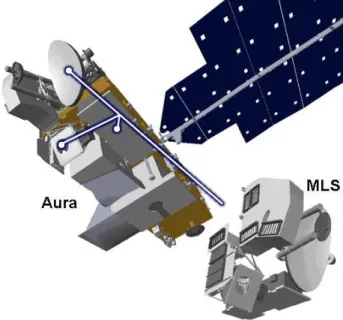
5.3 EOS MLS on AURA . . . 29
5.4 The limb sounding technique by MLS . . . 30
5.5 The limb sounding technique by MIPAS . . . 31
5.6 Atmospheric sounding . . . 32
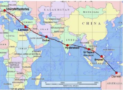
6.1 SCOUT-O3 Tropical Aircraft Campaign route . . . 36
6.2 SCOUT-AMMA Campaign route . . . 38
6.3 West African Monsoon . . . 39
6.4 The cost function evolution, case SCOUT-O3-1 . . . 42
6.5 The cost function evolution, case SCOUT-AMMA-3 . . . 43
6.6 The cost function evolution, case SCOUT-AMMA-2 . . . 44
6.7 SCOUT-O3-2 mean CRISTA-NF H2O profiles . . . 48
6.8 SCOUT-O3-2 mean MLS H2O profiles . . . 49
iv LIST OF FIGURES
6.9 SCOUT-O3-2 mean MLS O3 profiles . . . 50
6.10 SCOUT-O3-2 mean MLS HNO3 profiles . . . 51
6.11 SCOUT-O3-2 mean HALOE H2O profiles . . . 52
6.12 SCOUT-O3-2 mean HALOE O3 profiles . . . 52
6.13 SCOUT-O3-1 mean MIPAS-IMK H2O profiles . . . 53
6.14 North-south cross-sections of the zonal wind u component. . . . 54
6.15 MLS H2O analysis and control run for 4 November 2005 . . . . 55
6.16 CRISTA-NF H2O analysis increment and observations for 4 November 2005 . . . 55
6.17 MLS O3 analysis and observations for 4 November 2005 . . . 56
6.18 SCOUT-AMMA-3 CRISTA-NF H2O Profiles along the flight route . . . 57
6.19 SCOUT-AMMA-3 CRISTA-NF O3 Profiles along the flight route 58 6.20 SCOUT-AMMA-2 mean CRISTA-NF H2O profiles . . . 59
6.21 SCOUT-AMMA-3 mean CRISTA-NF O3 profiles . . . 60
6.22 SCOUT-AMMA-2 mean MLS H2O profiles . . . 61
6.23 SCOUT-AMMA-3 mean MLS O3 profiles . . . 62
6.24 SCOUT-AMMA-3 mean MLS HNO3 profiles . . . 63
6.25 SCOUT-AMMA-3 mean CRISTA-NF HNO3 profiles . . . 64
6.26 Zonal wind for 13 August 2006 . . . 65
6.27 CRISTA-NF H2O analysis increment and observations for 13 August 2006 . . . 65
6.28 MLS H2O analysis increment and observations for 13 August 2006 . . . 66
6.29 H2O analysis for 13 August 2006 . . . 66 6.30 SCOUT-AMMA-2 CRISTA-NF H2O profiles from 29 July 2006 67 6.31 SCOUT-AMMA-2 CRISTA-NF H2O profiles from 1 August 2006 68
List of Tables
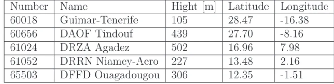
5.1 List of the radiosonde stations used in this work . . . 33
6.1 SCOUT-O3 Campaign flights . . . 37
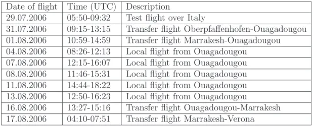
6.2 SCOUT-AMMA Campaign flights . . . 38
6.3 BECM parameter settings. . . 40
6.4 The system set-ups for different test cases. . . 40
A.1 Coefficients defining the vertical grid . . . 73
A.2 Photolysis reactions included in the model CHEM51 . . . 76
A.3 Gas phase reactions included in the model CHEM51 . . . 77
A.4 Heterogeneous reactions included in the model CHEM51 . . . . 81
CHAPTER
1
Introduction
Chemical weather forecasting (CWF) - a new field of atmospheric modelling - quickly developing and growing (Lawrence et al. [2005]). Many experimental studies (Rosenfeld[2000];Lohmann and Feichter[2005];Ramanathan and Feng [2009]) and numerical research simulations (Jacobson[2002];Grell et al.[2004]) show that atmospheric processes (meteorological weather, including the precip- itation, thunderstorms, radiation budget) depend on concentrations of chem- ical components in the atmosphere. CWF is closely related to the numerical weather prediction (NWP). The provision of all initial state conditions for model is crucial, in order to obtain a skillful numerical forecast (Elbern et al.
[2000]). For this purpose, NWP uses sets of sparse and spatially scattered weather observations to derive an objective analysis or data assimilation of the atmospheric state on model grids (Daley [1993]). According to Talagrand [1997], the termdata assimilation means ”using all the available information, to determine as accurately as possible the state of the atmospheric (or oceanic) flow.“ Thus, numerical model can promote valuable information to the analy- sis process, as it contains the fundamental physical laws of the atmospheric flow.
Stratospheric processes and their role in climate became more important for understanding the earth system research in recent past. The discovery of the ozone hole in the 1980s (Solomon [1988]) and its impact on human health (McMichael and Woodruff [2005]) led to additional interest in studying the interaction complexity between chemistry, radiation, and dynamics within the
2 Introduction
stratosphere. Further, the stratosphere holds the signature of anthropogenic forcing through the processes related to ozone depletion and increased green- house gas concentration (Dall’Amico et al. [2010]). In recent years, there has been increasing evidence that the stratosphere can influence tropospheric cli- mate from the tropopause down to the surface (Baldwin and Dunkerton[1999];
Thompson and Solomon [2002]).
Until the eighties only sparse observational data was available in stratosphere.
With the advent of space borne remote sounding devices, information about stratospheric trace gases can be retrieved from emitted, scattered, or trans- mitted radiation, which is recorded by these instruments. Presently, this in- struments are delivering an unprecedented wealth of observations of a number of stratospheric trace gases with global coverage. Among them is the Earth Observing System (EOS) Microwave Limb Sounder (MLS), an instrument on the NASA’s EOS Aura satellite, launched in July 2004 (Waters et al. [2004]).
In March 2002 the European research satellite ENVISAT was launched into a polar orbit carrying the Michelson Interferometer for Passive Atmospheric Sounding (MIPAS) aboard (Fischer et al. [2008]). Since January 2005, MI- PAS is providing measurements at a reduced spectral resolution (von Clarmann et al. [2009]). On board of the Upper Atmosphere Research Satellite (UARS) the Halogen Occultation Experiment (HALOE) was providing a long term re- cords of important stratospheric constituents in period from October 1991 to November 2005 (Nazaryan et al. [2005]).
The Upper Troposphere Lower Stratosphere (UTLS) is the transition layer between the stratosphere and the troposphere and is important for the trace gas exchange (Holton et al. [1995]). The UTLS area is marked by a strong spatial and temporal variability of the dynamic structures, often organized as filaments (Mahlman [1997]). This variability is controlled by transport and chemical transformation processes of trace gas distribution in this region (Riese et al.[2012]). In particular the modeling of water vapor in the UTLS is problematic, due to extremely strong gradient of the water vapor concentration there (Dee and Da Silva [2003]). Despite all, UTLS region is still sparsely covered by in situ measurements and not well resolved by satellite observations (Randel and Jensen [2013]).
The Cryogenic Infrared Spectrometers and Telescope for the Atmosphere -New Frontiers (CRISTA-NF) is an instrument developed in cooperation by Institute of Energy and Climate Research - Stratosphere, Research Centre Julich (IEK- 7) and University of Wuppertal. It is based on the satellite instrument CRISTA developed for studies of small-scale structures in atmospheric trace gas distri- butions. CRISTA participated in two Space Shuttle flights in November 1994 and August 1997 (Offermann et al. [1999]). Later, the center telescope of
3
CRISTA was adapted for use in the high-flying Russian research aircraft M55 Geophysica (Stefanutti et al. [1999]) and was termed CRISTA-NF (Schroeder et al.[2009]). Whereas the satellite observations are scattered and have a lim- ited resolution in space or time, the aircraft measurements, highly resolving and well suited for UTLS filamental structures, are of most interest for local studies. Two measurement campaigns, with CRISTA-NF on board of M55 Geophysica, took place within the remote sensing experiments: SCOUT-O3 and SCOUT-AMMA, over the periods November-December 2005 and July- August 2006 (Hoffmann et al. [2009];Weigel et al. [2010];Cairo et al.[2010]).
SCOUT-O3 was a measurement campaign in Darwin to study the transport of trace gases with high spatial resolution through the Tropical Tropopause Layer (TTL) (Hoffmann et al. [2009]). SCOUT-AMMA was a measurement campaign in west Africa with main objective to better document specific dy- namical and chemical processes and weather systems at various key stages of the monsoon season in TTL (Janicot et al.[2008]).
The state of the art aircraft instrument is the Gimballed Limb Observer for Radiance Imaging of the Atmosphere (GLORIA) (Riese et al. [2014]). While CRISTA-NF looks from the starboard side of the aircraft in a limb view- ing mode, GLORIA is designed to provide information by two- and three- dimensional observations with higher spatial resolution.
The observations, by nature, are scattered in space and time, while most ap- plications require spatially and temporally uniform and consistent fields of atmospheric constituents. Among these applications are operational weather forecasting (Geer et al.[2006]), ozone forecasting (Eskes et al.[2004]), process studies (Hoffmann and Riese[2004]), and initialization of climate models. Ap- plying the advanced data assimilation techniques (Kalnay [2003]), draws full advantage from stratospheric remote sounding data and UTLS in situ meas- urements.
The constituent data assimilation is less mature than meteorological data as- similation (Lahoz and Errera [2010]). Similar to NWP, stratospheric CWF is primarily an initial value problem, although the sources and sinks of chemical constituents have to be considered. Chemical equation systems are stiff, as a consequence of reaction rates, that vary by several orders of magnitude. This leads to strong error correlations between the species and can cause error cov- ariance matrices to become singular (Lahoz et al. [2007]). Thus, sophisticated numerical solvers, called stiff solvers, have to be used. The dimensionality of stratospheric CWF models is much higher than that of the NWP models.
Whereas the NWP models use under a dozen variables, the CWF model can have up to 100 different species, i.e., variables per grid point. This can result in univariate background error covariance matrix of size 1010, where the correct
4 Introduction
parametrisation has to be applied (Elbern et al. [2010])
Synoptic Analysis of Chemical constituents by Advanced Data Assimilation (SACADA) is a four-dimensional variational (4D-Var) assimilation system de- veloped for estimation of transport and chemical transformation of atmospheric trace gases in stratosphere (Elbern et al.[2010]). A key issue of this work was to adapt the SACADA assimilation system for the assimilation of high resolu- tion aircraft measurements. Model grid refinement, full revision and extension of chemical mechanism was therefore performed.
The main objectives of this thesis addresses the following questions:
1. What is the added value of assimilation of aircraft data compared to satellite data in UTLS region?
2. How performs data assimilation to the analysis and day prediction im- provement?
3. Is the resolution of SACADA assimilation system sufficient to assimilate aircraft data?
This thesis is organized as follows: The theory of chemical data assimilation is presented in chapter 2. The SACADA assimilation system, with its main components is described in chapter 3. The chapter 4 include theory and current setup of the BECM. A comprehensive set of case studies has been accomplished to evaluate and test the SACADA assimilation system. Profiles of various stratospheric trace gases derived from EOS MLS spectra as well as profiles of aircraft measurements from CRISTA-NF have been assimilated. Observational data from the HALOE and MIPAS-IMK satellite instruments and radiosondes served as an independent control data sets. Chapter 5 provides an overview of these instruments and the respective data products. The results are presented in Chapter 6. A summary of the present work as well as the final conclusions are given in Chapter 7.
CHAPTER
2
Data assimilation
The main goal of data assimilation is coupling of the observed information with our theoretical knowledge as given by models, to obtain most probable system state at a given time. In meteorology, for instance, it is important to have an optimal state estimation of the atmosphere and evolution for improved forecasts. Since probability theory is one of the guiding basis for the data assimilation, a short description is presented here.
2.1 Bayes’ theorem
Assume that a probability density function (PDF) p(x), p : Rn → R of the discrete approximation of the atmospheric statex is available, called a priori probability. In addition information provided by the observations y ∈ Rp are given with the error characteristics. Thus, it is possible to formulate a PDF p(y|x), which describes the probability of takingy measurements under a given atmospheric statex. Then thea posteriori PDFp(x|y) can be derived by Bayes’ theorem as follows:
p(x|y) = p(y|x)p(x)
R p(y|x)p(x)dx. (2.1.1)
6 Data assimilation
2.2 Maximum likelihood and minimum vari- ance
Consider a case of two independent observations y1 and y2. Their errors are assumed to be normally distributed with standard deviations σ1 and σ2, re- spectively. Define xa as the analysis of the most likely state of x under con- dition of the given observations. Then the probability distribution to measure y1 under condition of a given true state x is written as
p(y1|x) = 1
√2πσ1 exp
−(y1−x)2 2σ21
. (2.2.1)
Further, the likelihood of a true state xunder condition of the given observa- tions y1 and y2 with standard deviations σ1 and σ2 are given by
L(x|y1) =p(y1|x) = 1
√2πσ1
exp
−(y1−x)2 2σ12
L(x|y2) =p(y2|x) = 1
√2πσ2 exp
−(y2−x)2 2σ22
,
respectively.
Hence, the most likely state of x under conditions of the given independent observations y1 and y2 is the maximum of the joint probability:
maxx L(x|y1, y2) = p(y1|x)p(y2|x) = 1
2πσ1σ2
exp
−(y1−x)2
2σ12 −(y2−x)2 2σ22
, (2.2.2) which is similar to the maximum of the negative logarithm
maxx lnL(x|y1, y2) = max
x {const.−J(x)}. (2.2.3) Thereby,
J(x) = 1 2
(x−y1)2
σ21 +(x−y2)2 σ22
= 1
2
x−y1
x−y2
T σ12 0
0 σ22 −1
x−y1
x−y2
(2.2.4)
2.3 Four-dimensional variational data assimilation 7
is the cost function. Hence, the maximum likelihood is obtained if the cost function (2.2.4) is minimized. The minimum of the cost function is called the best linear unbiased estimate (BLUE).
2.3 Four-dimensional variational data assimil- ation
Four-dimensional variational data assimilation (4D-Var) allows to use obser- vations distributed not only in space but also in time. The main goal of the 4D-Var is to optimise a state of the atmospherex0 for the timet0 (first guess), so that the model analysis (forecast) started with this state M(x0) for time interval (t0, tN) is as close as possible to all observations (y1, . . . , yp) scattered in this time interval and to the background (a-priori) informationxb. A-priori information can be the result of a previous analysis, climatological statistics, a model forecast or some combination of those.
Generalising (2.2.4) the cost function for this problem is written as follows J(x0) = Jb+Jo =
= 1
2[x0−xb]TB−1[x0−xb] + 1
2
p
X
i=0
[H(Mi(x0))−yi]TR−1[H(Mi(x0))−yi]. (2.3.1)
HereR(a matrix of sizep×p) andB (a matrix of sizen×n) are the observation and background error covariance matrices, respectively and H (a matrix of size p×n) is the projection operator that maps the state vector from the m- dimensional model space on the p-dimensional observation space. Mi is the model operator generating the state xi at time step ti as a function of x0. The first term of the cost function (2.3.1) quantifies the distance between the background state and the first guess at the beginning of the time interval. The second term describes a sum of the distances between each observationyi and the corresponding model state H(Mi(x0)) for the moment of observation.
Efficient minimisation algorithms like quasi-Newton or Conjugate-Gradient methods require the gradient of the cost function with respect to the con- trol variables x0 in order to find the minimum of J. The gradient of the cost function background partJb is obtained by
∇x0Jb =B−1
x0−xb
. (2.3.2)
8 Data assimilation
On the contrary, the gradient of the observational cost function part Jo with respect to the initial model values is more difficult to calculate. However, it is easy to express the gradient of Jo with respect to the model variables at the time ti, namely
∇xiJo =H′TR−1[H(xi)−yi] . (2.3.3) The calculation of ∇x0Jo is computationally the most demanding task of 4D- Var. Since the number of control variables in atmospheric models is of the order 106–107, the only feasible strategy to accomplish this calculation is given by utilising the adjoint model operator.
Leth·, ·ibe the canonical scalar product. Then, the variation of a scalar func- tion f :Rn→R in response to a small variationδxof xcan be approximated to the first order by
δf ≈ h∇xf , δxi .
Due to the linearity of the scalar product, the variation of Jo is given by δJo ≈
N
X
i=0
h∇xiJo , δxii , (2.3.4)
where δxi :=Mi(x0+δx0)−Mi(x0)≈M′iδx0.
In other words, δxi is linked to the variation of the initial model values δx0
by the tangent linear model M′, Which is the Jacobian of the model operator M. Using (2.3.4), the variation of the cost function can be expressed as
δJo ≈
N
X
i=0
h∇xiJo , M′iδx0i =
N
X
i=0
hM∗i∇xiJo , δx0i . (2.3.5) M∗ is the adjoint model operator, which is the transpose of the tangent linear M′ (see Talagrand and Courtier [1987] for a detailed discussion).
By combining (2.3.5) and (2.3.3), the gradient ofJo with respect to the initial model values x0 can be determined as
∇x0Jo =
N
X
i=0
M∗i∇xiJo =
N
X
i=0
M∗iH′TR−1[H(xi)−yi] .
Hence, the complete gradient of the cost function with respect to the control variables x0 can be written as
∇x0J =B−1
x0−xb +
N
X
i=0
M∗iHTR−1[H(xi)−yi] . (2.3.6)
2.3 Four-dimensional variational data assimilation 9
2.3.1 Adjoint model technique
A numerical model integration over a time interval [t0, ti] is subdivided into a number of time-steps:
xi =Mi,i−1◦ · · · ◦M2,1◦M1,0(x0).
Accordingly, the tangent linearM′i of this sequence of model operators is given by
M′i =M′i,i−1· · ·M′2,1M′1,0.
Since the model is non-linear, each of the linearized operatorsM′l,l−1 explicitly depends on the current atmospheric statexl−1. In order to obtain the adjoint model operator by forming the transpose of the tangent linear, the sequence of operators is reversed:
M∗i =M∗1,0· · ·M∗i−1,i−2M∗i,i−1.
Thus, the adjoint model operator M∗i propagates the gradient of the cost function with respect toxi backward in time, to deliver the gradient of the cost function with respect to x0. Taking into account that each adjoint operator M∗l,l−1 depends on xl−1, the sequence of atmospheric states must be available in reverse order for each time-step. To this end, all intermediate model states xl must be stored forl= 0,· · · , iduring the forward integration of the model M. Alternatively, they have to be recomputed during the course of adjoint integration.
The adjoint model can be created from the computer code implementing the model M. By examining the whole program unit in reverse order, the adjoint code can be constructed statement by statement. A detailed description of this technique is given in Giering and Kaminski [1998]. Obviously, this approach is error-prone for comprehensive atmospheric models, with thousands of code lines. However, the hard coding work can be alleviated by partly automated using of adjoint compilers like TAMC (Giering [1999]) or Tapenade (Hasco¨et and Pascual [2004]).
CHAPTER
3
The SACADA assimilation system
SACADA, Synoptic Analysis of Chemical constituents by Advanced Data As- similation, is a four-dimensional variational assimilation system developed for the estimation of transport and chemical transformation of atmospheric trace gases in the stratosphere (Elbern et al. [2010]). The version developed in this study is designed to analyze two aircraft-based measurement campaigns, SCOUT-O3 and AMMA, over the periods November-December 2005 and July- August 2006, respectively (Hoffmann et al. [2009], Weigel et al. [2010]; see chapter 6 for more details).
A key issue of this work was to adapt the SACADA assimilation system for the assimilation of high resolution aircraft measurements. Therefore, a model grid refinement and an extension of the chemical mechanism are undertaken. This chapter gives an overview of the main components of the SACADA system, such as the model operator M, including the chemistry transport module for solving a system of chemical reactions and its adjoint. The meteorological module, the grid configuration and the parallelization technique are adopted from the global numerical weather prediction model (GME) of the German Weather Service (Majewski et al.[2001a]).
12 The SACADA assimilation system
3.1 The SACADA model
Within SADACA the atmospheric state is described by a system of partial differential equations (PDEs), where the temperature T, pressure p, the hori- zontal wind field v, the density of the air parcel ρ, the mixing ratio of water in its various phasesq and the mixing ratios c of trace gases are given by (see e.g. Kalnay [2003])
dv
dt =−α∇p− ∇φ+F −2Ω×v (3.1.1a)
∂ρ
∂t =−∇(vρ) (3.1.1b)
∂q
∂t =−v∇q+ (E−C) (3.1.1c)
∂c
∂t =−v∇c+ (P −L) (3.1.1d)
Q=Cp
dT
dt −αdp
dt. (3.1.1e)
Here, φ is the geopotential, α is the specific volume of air (the inverse of the density ρ),Ωis the angular velocity of the Earth andF is the frictional force.
Equation (3.1.1a) represents the conservation of momentum, equation (3.1.1b) denotes the conservation of mass. The equation (3.1.1c) describes change of water vapor mixing ratio in time (t) withEandC denoting the rate of change due to liquid, solid and gas phase transitions. Equation (3.1.1e) represents con- servation of energy with the rate of heating Q. Equation (3.1.1d) is solved by the chemistry transport module of the SACADA model, later called SACADA- CTM, using the precomputed meteorological fields. P andLare representing for the chemical production and loss, respectively. Equations (3.1.1c) and (3.1.1e) are solved by the German Weather Service’s global forecast model GME, which serves as meteorological driver. GME is coupled online with SACADA, thus, both models share the same grid resolution.
SACADA has to comply with several requirements, such as to be efficient in order to deliver analyses in near real-time. Another requirement concerns the model error, which should be kept as small as possible, as in 4D-varM is con- sidered to be perfect. The benefit of having the meteorological model included in assimilation system is that interpolation errors of the meteorological fields such as wind and temperature on the model grid can be avoided, as in this case both modules are using the same grid. SACADA is the first 4D-var stra- tospheric constituent data assimilation model that combines a comprehensive stratospheric chemistry module and a meteorological model.
3.2 Chemistry transport module 13
The icosahedral grid adopted from GME is one of the essential benefits in the SACADA system. The main advantage of the icosahedral-hexagonal grid, in comparison to traditional grid structures like latitude-longitude grids, is a rather small variability of the area of grid cells, as the well-known pole-problem of the latitude-longitude grid does not exist while using the GME grid (Kalnay [2003]).
3.2 Chemistry transport module
In the framework of this study, the chemistry transport module of SACADA as- similation system was improved. The chemistry mechanism was revised and all reaction rates were updated according to Jet Propulsion Laboratory (JPL) re- commendations. Thus, a novel global chemistry transport model (CTM) with its adjoint version is now the kernel of SACADA system. The new chemistry mechanism and its adjoint was tested according toChao and Chang[1992]. In this section the principal features of the chemistry mechanism are described.
The SACADA-CTM solves equation (3.1.1d). An operator splitting approach (McRae et al. [1982]) is used to obtain the discrete approximate solution of this partial differential equation. The PDE is splitted into three sub-problems, written in the local coordinate system of the icosahedral grid (Schwinger [2006]), such as
∂c
∂t h
=− u RE
∂c
∂η − v RE
∂c
∂χ, (3.2.1a)
∂c
∂t v
=−w∂c
∂p, (3.2.1b)
∂c
∂t c
= (P −L). (3.2.1c)
These equations describe the temporal evolution in the volume mixing ratio due to horizontal advection (3.2.1a), vertical advection (3.2.1b) and chemical production and loss (3.2.1c), denoted by the superscripts h, v, and c, respect- ively.
Different numerical schemes are used to discretise and solve each of these equa- tions. As the chemical differential equations are stiff, the implicit scheme with an adaptive step size control is used for solving them. Thus, the concentrations on time-steptn+1 are obtained by
14 The SACADA assimilation system
c(tn+1) =
Mc(tn)◦Mv(tn)◦Mh(tn)
c(tn−1). (3.2.2) Here, Mc, Mv and Mh are discrete operators that solve (3.2.1a) – (3.2.1c). In order to calculate concentrations at time-step tn+1 from time-step tn−1, the meteorological information on time-steptnis used. Hence, equation (4.10) de- scribes a forward time stepping using twice the meteorological time step, where the meteorological data are at the center of the time interval. An advantage of this kind of approach is the reduction of levels, where the field of chemical constituents have to be stored, for using them in adjoint computations.
Chemistry scheme and solver
The chemical reaction mechanism of SACADA-CTM was revised and exten- ded. All reaction rates were updated according to the recommendations of the JPL (Sander et al. [2011]). The current SACADA-CTM includes a set of 49 photolysis reactions, 138 gas phase reactions and 10 heterogeneous reactions on surfaces of Polar Stratospheric Cloud (PSC) particles and in sulphate aer- osol droplets. The reaction equations together with their rate constants are listed in Tables A.2, A.3 and A.4.
The kinetic preprocessor (KPP) is a software tool that assists the com- puter simulation of chemical kinetic systems (Sandu et al. [2003]). KPP is used to construct a module solving equation (3.2.1c) for each grid cell. The chemical reaction mechanism of SACADA is formulated in the special KPP language and the KPP generated source code inFortran, with some additional modifications, is implemented in SACADA assimilation system.
The numerical solution of equation (3.2.1c) is obtained by a second order Rosenbrock method (Verwer et al. [1997]). It is a two stage linear-implicit scheme. For an arbitrary autonomous differential equationdx/dt=f(x) with f :Rm→Rm the Rosenbrock method reads as:
x(t+τ) =x(t) + 3
2τk1 +1
2τk2, (3.2.3)
and the coefficients k1 and k1 are obtained from (I−γτJ)k1 =f(x(t))
(I−γτJ)k2 =f(x(t) +τk1)−2k1, (3.2.4) whereγ = 1 + 1/√
2 andτ is the step length,I andJare identity and Jacobian matrices, respectively. (Verwer et al. [1997],Sander et al. [2003]).
3.3 The adjoint model 15
The Tropospheric Ultraviolet-Visible (TUV) Radiation Model is a radi- ation transfer model developed at the Atmospheric Chemistry Division of US National Center for Atmospheric Research (NCAR), which calculates spec- tral irradiances, spectral actinic fluxes, and photo-dissociation rates for the wavelength range between 120 and 735 nm. The TUV Version 4.2 is ad- apted to the SACADA model in order to build a look-up table of photo- dissociation frequencies for the stratospheric SACADA assimilation system (Schwinger [2006]). The look-up table contains photolysis rates J(z, co, φ) for different values of the zenith angleφ, the overhead ozone columnco, dependent on the altitude z as defined by the vertical SACADA model grid. Note that co is defined as a factor, which describes an enhancement or reduction of a standard ozone column. In the framework of this work the TUV SACADA model is revised, all cross section input data is updated according to the re- commendations issued by the JPL and the new look-up table is built for a refined SACADA model grid.
3.3 The adjoint model
To calculate the gradient of the cost function with respect to the initial con- centrations ∇c0J the adjoint of the model operator M∗ is needed (see Equa- tion 2.3.6). The transpose of the tangent-linear (or Jacobian) of the operators Mh is obtained by forming the tangent-linear of each individual line of code and transposing it, as described by Giering and Kaminski [1998]. The ad- joint ofMc is provided by KPP using the adjoint of the Rosenbrock numerical scheme (Sandu et al. [2005]). As the operator Mv is linear, the Jacobian
∂Mv
∂c = [I+ 2∆tA]−1
is the operator itself and hence, the adjoint is the simple transpose Mv∗ = [I+ 2∆tA]−T .
The values for the recomputation of the required variables for Mc∗ and Mh∗ are saved to disk at each time step. Thereby, the volume mixing ratios are applied before the respective model operator.
During the adjoint model integration, the gradient of the observational cost function part is added to the adjoint variable ˜c∗(tn+1). Thereby observations yn+1 within the time interval [tn, tn+2] are taken into account. Then ˜c∗(tn+1)
16 The SACADA assimilation system
is propagated backward in time by means of the adjoint model:
c∗(tn+1) = ˜c∗(tn+1) +HTR−1[yn+1−Hc(tn+1)]
c∗(tn−1) = [Mh∗◦Mv∗◦Mc∗]c∗(tn+1) (3.3.1) Finally, at n− 1 = 0, the gradient of Jo with respect to the initial volume mixing ratios c(t0) is obtained:
∇c0Jo =c∗(t0).
3.4 Meteorological module, grid configuration and parallelization
The German Weather Service global forecast model GME, which is the first operational meteorological model utilizing an icosahedral grid structure, was made available (model version 1.22) and serves as the meteorological driver module in the SACADA assimilation system. Since the new parts of the SACADA model, which are developed in the framework of this study, include improvement of the icosahedral GME grid, the principal features of GME is presented in this section. For a more detailed description of the GME model, the reader is referred to Majewski et al.[2001b].
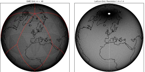
Figure 3.1: Icosahedral grid with a resolution of ni = 48 (left). The distance between neighboring grid points is about 147 km. The boundaries of diamonds (see text) are marked by red lines. A conventional latitude-longitude grid with a resolution of 1.4o×1.4o for comparison (right).
3.4 Meteorological module, grid configuration and parallelization 17
To generate the icosahedral-hexagonal grid, a regular icosahedron, the highest Platonic body with 20 equilateral triangles, is constructed inside the sphere such that two of its twelve vertices coincide with the North Pole (NP) and South Pole (SP), respectively. The resulting sections of great circles (or sides of the triangles), are equally subdivided into a number of ni intervals each.
Thus, each of the triangles are devided in n2i sub-triangles. As shown in the upper graphic of Figure 3.1, the constructed grid is almost isotropic. Each grid point has six nearest neighbors with the exception of twelve points located at the vertices of the original icosahedron (called special points hereafter), which have only five direct neighbors. The area of representativeness for a grid cell is a hexagon and pentagon at the twelve special points, respectively (see Figure 3.2).
5
P 3
1 2 6
4
1
2
3 5 4
P
Figure 3.2: The icosahedral grid cells geometry. The area of representativeness assigned to each grid cell is a hexagon or a pentagon at the twelve special points, respectively.
This approach of the grid structure results in a mesh with virtually constant mesh size all over the globe. Thereby the minimum and maximum separation between neighboring grid points ∆min and ∆max varies about 20% only. For the SACADA system in this study it has been decided that ni = 48 gives a sufficient resolution, resulting in 23 042 grid points per level. The minimum and maximum distances are ∆min = 147 km and ∆max= 176 km, and the av- erage area of representativeness is about 24 000 km2. A comparable traditional latitude-longitude grid (lower graphic of Figure 3.1), that is a grid with the same area represented by one grid cell at the equator (where the resolution is coarsest), requires a grid spacing of 1.4o ×1.4o. This results in 33 024 grid points per level, which is about 40% more than the icosahedral grid. To obtain a rectangular data structure for the icosahedral grid, two adjacent spherical triangles are combined to form a diamond, partitioning the grid into ten lo-

![Figure 3.4: Domain decomposition for six processors. Each color indicates a region that is assigned to one processor (Schwinger [2006]).](https://thumb-eu.123doks.com/thumbv2/1library_info/3693431.1505672/29.892.312.577.730.1007/figure-domain-decomposition-processors-indicates-assigned-processor-schwinger.webp)
![Figure 5.4: Illustration of the limb sounding technique by MLS. From Waters et al. [2004]](https://thumb-eu.123doks.com/thumbv2/1library_info/3693431.1505672/40.892.157.747.258.542/figure-illustration-limb-sounding-technique-mls-waters-et.webp)