Four-dimensional variational data
assimilation for estimation of the atmospheric chemical state from
the tropopause to the lower mesosphere
I n a u g u r a l – D i s s e r t a t i o n zur
Erlangung des Doktorgrades
der Mathematisch–Naturwissenschaftlichen Fakult¨ at der Universit¨ at zu K¨ oln
vorgelegt von
J¨ org Schwinger
aus Bonn
K¨ oln 2006
Berichterstatter: Prof. Dr. A. Ebel
Prof. Dr. M. Kerschgens
Tag der m¨ undlichen Pr¨ ufung: 30.10.2006
Abstract
A four-dimensional variational data assimilation system for stratospheric trace gas observations has been developed and operated. The system of- fers the flexibility to make use of data from different instruments and it was designed (1) to enforce chemical consistency by constraining the analyses to a state of the art stratospheric model, (2) to provide realistic estimates of anisotropic and inhomogeneous background error covariances, and (3) to be sufficiently efficient for application in near real time. The assimilating model has been assembled from scratch to allow for a couple of novel features:
The meteorological fields are computed online by the global forecast model
GME of German Weather Service, leading to an improved numerical repre-
sentation of wind fields compared to traditional offline chemistry-transport
models, which use spatially and temporally interpolated meteorological anal-
yses. A number of 155 photolysis, gas phase, and heterogeneous reaction of 41
stratospheric trace gases is considered by the chemistry module. Since spatial
correlations between background errors evolve according to the atmospheric
flow, a flow dependent formulation of the background error covariance ma-
trix has been devised by means of a diffusion approach. It can be shown
that this measure considerably improves the analysis quality particularly in
regions where large gradients of potential vorticity prevail. The governing
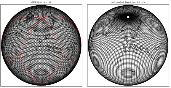
equations are discretised on an icosahedral grid, as this significantly reduces
the computational cost. Therefore, it is possible to operate the model with
a relatively fine spatial resolution without violating the near real time con-
straint. A comprehensive set of case studies has been conducted in order
to test and evaluate the new system. Trace gas profiles derived from mea-
surements of the Michelson Interferometer for Passive Atmospheric Sounding
(MIPAS) have been assimilated. Comparison with independent (not assimi-
lated) control data sets and statistical evaluation demonstrates an excellent
performance of the new assimilation system.
Kurzzusammenfassung
Ein System zur Assimilation stratosph¨ arischer Spurengasmessungen basie-
rend auf der vierdimensionalen variationellen Methode wurde entwickelt und
angewandt. Dieses neue System bietet die M¨ oglichkeit, Messdaten verschie-
denster Sensoren zu verwenden, und zeichnet sich durch (1) chemische Kon-
sistenz der analysierten Felder im Sinne eines umfassenden stratosph¨ arischen
Modells sowie (2) realistische Modellierung von anisotropen und inhomoge-
nen Hintergrundfehler-Kovarianzen aus und erm¨ oglicht (3) aufgrund seiner
hohen nummerische Effizienz einen operationellen Einsatz. Das f¨ ur die Assi-
milation verwendete Modell wurde neu entwickelt und weist eine Reihe von
vorteilhaften Eigenschaften auf. Die meteorologischen Felder werden mithil-
fe des globalen Wettervorhersagemodells GME des Deutschen Wetterdiens-
tes direkt erzeugt. Dadurch wird, im Vergleich zu herk¨ ommlichen Chemie-
Transport-Modellen, die zeitlich und r¨ aumlich interpolierte meteorologische
Analysen verwenden, die Darstellung der Windfelder im Modell entscheidend
verbessert. Das Chemiemodul ber¨ ucksichtigt 155 Photolyse-, Gasphasen-,
und heterogene Reaktionen zwischen 41 stratosph¨ arischen Spurengasen. Da
die r¨ aumlichen Korrelationen von Hintergrundfehlern an die Dynamik der
atmosph¨ arischen Str¨ omung gekoppelt sind, wurde eine str¨ omungsabh¨ angige
Formulierung der Hintergrundfehler-Kovarianzmatrix mithilfe eines Diffusi-
onsansatzes realisiert. Es l¨ asst sich zeigen, dass dadurch die Qualit¨ at der Ana-
lysen deutlich verbessern werden kann, insbesondere in Gebieten, in denen
die potentielle Vorticity starke Gradienten aufweist. Die L¨ osung der Modell-
gleichungen erfolgt auf einem Ikosaedergitter, durch dessen Verwendung der
Rechenaufwand signifikant verringert wird. Aus diesem Grund ist es m¨ oglich,
das Modell auch im operationellen Einsatz mit einer relativ hohen r¨ aumlichen
Au߬ osung zu betreiben. Anhand von umfangreichen Fallstudien konnte das
neue System getestet und evaluiert werden. Dazu wurden Spurengasprofile,
abgeleitet aus Messungen des Michelson Interferometer for Passive Atmo-
spheric Sounding (MIPAS), assimiliert. Vergleiche mit unabh¨ angigen (nicht
assimilierten) Beobachtungen und statistische Auswertungen zeigen, dass das
neue Assimilationssystem hervorragend arbeitet.
Contents
1 Introduction 1
2 Data assimilation and the 4D-var technique 7
2.1 Maximum likelihood and minimum variance estimates . . . . . 8
2.2 Four-dimensional variational data assimilation . . . 10
2.2.1 Properties of the adjoint model . . . 12
3 Background error covariances 15 3.1 An incremental formulation of the cost function . . . 18
3.2 Correlation modelling using a diffusion approach . . . 19
3.2.1 Discrete formulation . . . 21
3.2.2 Three-dimensional correlations . . . 23
3.3 Flow dependent inhomogeneous and anisotropic correlations . 25 3.3.1 The normalisation matrix . . . 26
4 Description of the SACADA assimilation system 29 4.1 The SACADA model . . . 29
4.1.1 Theoretical background . . . 31
4.1.2 Meteorological module, icosahedral grid and paralleli-
sation . . . 32
ii CONTENTS
4.1.3 Chemistry transport module . . . 36
4.2 The adjoint model . . . 44
4.3 BECM implementation . . . 44
4.4 Assimilation system set-up . . . 46
5 Observational basis 51 5.1 Retrieval methods . . . 52
5.1.1 Averaging kernels . . . 54
5.1.2 Assimilation of retrievals vs. assimilation of radiance . 55 5.2 Instrument and data product description . . . 57
5.2.1 MIPAS . . . 57
5.2.2 SCIAMACHY . . . 58
5.2.3 SAGE II and HALOE . . . 59
6 Case studies 63 6.1 System set-up . . . 66
6.2 General results . . . 67
6.3 Flow dependent BECM parameterisation . . . 76
6.4 Statistical evaluation and cross validation . . . 82
6.4.1 Ozone . . . 82
6.4.2 CH
4, N
2O, NO
2, H
2O and HNO
3. . . 96
6.4.3 Statistical evaluation . . . 106
7 Summary and Conclusions 109 A Vertical advection scheme: Implementation 113 B Implementation of diffusion schemes 117 B.1 Horizontal diffusion . . . 117
B.1.1 Transpose horizontal diffusion . . . 118
B.2 Vertical diffusion . . . 119
C Tables 121 C.1 Vertical grid parameters . . . 121
C.2 Reaction equations and rate constants . . . 123
CONTENTS iii
Acknowledgements 139
List of Figures
3.1 Effect of background error covariances on the analysis . . . 16
3.2 Potential vorticity and ozone fields for 28 October 2003 . . . . 27
4.1 Icosahedral grid vs. latitude-longitude grid . . . 32
4.2 Geometry of grid cells in the icosahedral grid . . . 33
4.3 Definition of local coordinates (η, χ) . . . 34
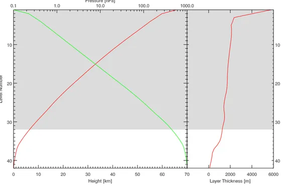
4.4 Pressure and height of SACADA model layers . . . 37
4.5 Domain decomposition and parallel speed-up . . . 38
4.6 Reference profiles of sulfate aerosol characteristics . . . 43
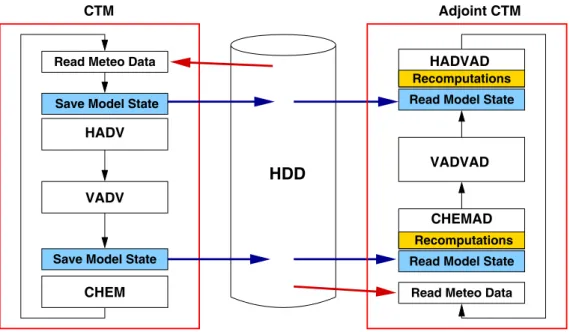
4.7 Storage strategy of the SACADA assimilation system . . . 45
4.8 Distribution of differences between random and exact normal- isation . . . 46
4.9 Example for a discrete correlation function modeled by means of the diffusion operator . . . 47
4.10 SACADA system set-up . . . 48
5.1 Limb viewing geometry of space borne remote sounding in- struments . . . 52
5.2 Averaging kernels for an O
3retrieval . . . 55
6.1 Data availability for the three case study periods . . . 65
LIST OF FIGURES v
6.2 CS3-MPI-1 cost function . . . 68
6.3 CS1-MPE-1 cost function . . . 69
6.4 CS2-MPE-1 cost function . . . 70
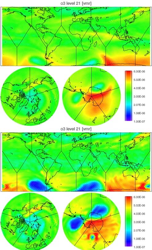
6.5 CS1-MPE-1 ozone analysis for 20 September 2002 . . . 72
6.6 CS1-MPE-1 ozone analysis for 25 September 2002 . . . 73
6.7 CS1-MPE-1 ozone analysis for 25 September 2002 . . . 74
6.8 CS1-MPE-4 ozone analysis for 20 September 2002 . . . 75
6.9 CS1-MPE-4 cost function . . . 76
6.10 PV-distribution at 27 October 2003 . . . 77
6.11 CS3-MPE-2 and CS3-MPE-3 ozone analysis, 27 October 2003 . . . 78
6.12 CS1-MPE-4 and CS1-MPE-5 ozone analysis, 13 September 2002 . . . 79
6.13 PV-distribution at 13 September 2002 . . . 80
6.14 Relative difference between the J
pfvalue for CS1-MPE-4 and CS1-MPE-5 . . . 80
6.15 Relative difference between the J
pfvalue for CS1-MPE-4 and CS1-MPE-5 (ozone only) . . . 81
6.16 CS1-MPI-1 mean MPI ozone profiles . . . 83
6.17 CS1-MPI-1 mean MPE ozone profiles . . . 84
6.18 CS1-MPI-1 mean HALOE ozone profiles . . . 85
6.19 CS1-MPI-1 mean SAGE II ozone profiles . . . 86
6.20 CS1-MPI-1 mean SCL ozone profiles . . . 87
6.21 CS1-MPI-1 mean SCO ozone profile . . . 88
6.22 CS2-MPE-1 mean MPE ozone profiles . . . 89
6.23 CS2-MPE-1 mean MPI ozone profiles . . . 90
6.24 CS2-MPE-1 mean HALOE ozone profiles . . . 91
6.25 CS2-MPE-1 mean SAGE II ozone profiles . . . 92
6.26 CS2-MPE-1 mean SCL ozone profiles . . . 93
6.27 CS2-MPE-1 ozone bias with respect to MPE observations . . 94
6.28 CS3-MPI-1 mean MPI CH
4profiles . . . 97
6.29 CS3-MPI-1 mean MPI N
2O profiles . . . 98
6.30 CS3-MPI-1 mean MPI HNO
3profiles . . . 99
vi LIST OF FIGURES
6.31 CS3-MPI-1 mean MPI H
2O profiles . . . 100
6.32 CS3-MPI-1 mean MPI NO
2profiles . . . 101
6.33 CS3-MPI-1 mean MPI nighttime NO
2profiles . . . 102
6.34 CS3-MPI-1 mean MPI NO
2daytime profiles . . . 103
6.35 CS3-MPI-1 bias of analysed NO
2against MPI observations at high northern latitudes . . . 104
6.36 CS3-MPI-1 bias of analysed NO
2against MPI observations at tropical latitudes . . . 105
6.37 CS3-MPE-2 O − B distribution for O
3. . . 106
6.38 CS2-MPI-1 O − B and distribution for N
2O, CFCl
2, N
2O
5, HNO
3, ClONO
2and O
3. . . 107
6.39 CS2-MPI-1 O − B distribution for CH
4, H
2O and NO
2. . . . 108
A.1 Definition of quantities for the vertical advection scheme . . . 113
List of Tables
5.1 Summary of MIPAS and SCIAMACHY data product charac-
teristics . . . 60
6.1 BECM parameter settings for different configurations of the assimilation system . . . 67
C.1 Coefficients defining the vertical grid . . . 121
C.2 Photolysis reactions included in the model . . . 123
C.3 Gas phase reaction equations and rate constants . . . 124
C.4 Heterogeneous reactions included in the model . . . 128
CHAPTER 1
Introduction
The term data assimilation originates from meteorology. With the advent of numerical weather prediction in the 1950s it became necessary to provide initial conditions for the computer models in order to obtain a numerical forecast. To this end, an objective analysis of the atmospheric state on regular model grids had to be derived from a set of sparse and spatially scattered weather observations. It soon became apparent that the numerical model can contribute valuable information to the analysis process, as it includes the physical laws governing the atmospheric flow. According to Talagrand [1997],
assimilation of meteorological or oceanographical observations can be de- scribed as the process through which all the available information is used in order to estimate as accurately as possible the state of the atmospheric or oceanic flow. The available information essentially consists of the ob- servation proper, and of the physical laws which govern the evolution of the flow. The latter are available in practice under the form of a numer- ical model.
Assimilation of atmospheric trace gas observations is closely related to me- teorological data assimilation, as the numerical models are similar in terms of complexity and the large dimension of the state vector.
Stratospheric processes have been recognised to be of utmost importance for
the earth system in recent years. The discovery of the ozone hole in the
1980s and, later on, the question how human activity influences the earth’s
2 Introduction
climate system has led to an increased interest in a thourough understanding of the complex interaction between chemistry, radiation, and dynamics of the stratosphere. Stratospheric trace gases play a key role in the radiation bud- get of the earth and their distribution influences the atmospheric circulation.
Conversely, atmospheric conditions determine the rate of chemical reactions as well as the redistribution of trace gases by advection and turbulent diffu- sion (World Meteorological Organization [1999], Intergovernmental Panel on Climate Change [2001]).
For a long time only sparse stratospheric observational data was available.
The lower stratosphere up to a height of approximately 32 km is being ob- served by a more or less dense network of ozone sondes, while for larger alti- tudes instruments mounted on research rockets were the only source of in situ observational data. With the advent of space borne remote sounding devices, information about stratospheric trace gases can be derived from emitted, scattered, or transmitted radiation, which is recorded by these instruments.
In March 2002 the European research satellite EnviSat was launched into a polar orbit carrying the Michelson Interferometer for Passive Atmospheric Sounding (MIPAS) and the Scanning Imaging Absorption Spectrometer for Atmospheric Chartography (SCIAMACHY) aboard, which are delivering an unprecedented wealth of observations of a number of stratospheric trace gases with global coverage.
However, satellite observations are, by nature, scattered in space and time, whereas the vast majority of applications require spatially and temporally uniform and consistent fields of atmospheric constituents. These applications include operational weather forcasting (e. g. Derber and Wu [1998], Geer et al. [2006]), ozone forecasting (Eskes et al. [2002], Eskes et al. [2004]), process studies (e. g. Hoffmann and Riese [2004]), and initialisation of climate models. Hence, advanced data assimilation techniques, must be applied to draw full advantage of stratospheric remote sounding data. For stratospheric constituent assimilation these techniques should ideally be able
1. to combine all available observational data from different sensors in an optimal way according to their error statistics, thereby
2. producing a comprehensive and chemically consistent picture of the atmospheric state, and
3. to reveal information about unobserved species, which are chemically coupled with observed constituents.
Furthermore, data assimilation can be used to identify inconsistencies be-
tween atmospheric models and observational data. It should be emphasised
3
that this task cannot be accomplished by comparing an unconstrained model integration with measurements, as even a perfect model is not expected to re- produce observations, unless adequate initial conditions are supplied. Hence, advancements in the understanding of atmospheric processes require a con- frontation of models with data by employing assimilation techniques, which are rigorously based on statistical theory. In this spirit, data assimilation has been used, for example, to test chemical theories (Lary et al. [2003]) and to monitor observation errors (Stajner et al. [2004]).
Data assimilation of stratospheric constituents is a complex and computa- tionally expensive endeavour. The elaborate model is only one part of the whole assimilation system and often considerable simplifications have been introduced in oder to reduce the computational cost. In this regard, the im- plementation of the background error covariance matrix (BECM) is a crucial issue: Since an optimal analysis requires a realistic representation of error statistics, the BECM constitutes a core element of the assimilation system.
Especially if data is sparse, the analysis quality largely depends on the back- ground error correlations encoded in the BECM. However, the dimension of this this matrix is enormous for comprehensive three-dimensional mod- els and, consequently, it can only be handled in parameterised form. As the background field is invariably given by a short range forecast in present assimilation systems, it is the error statistics of this forecast that is to be approximated. Several approaches to this problem with differing degrees of sophistication exist (see Riishøjgaard [1998] for a detailed discussion). De- spite the necessary simplicity, a skillful parameterisation should be capable of representing the relevant structures of the background error covariances. This includes the possibility of modelling inhomogeneous (varying with location) and anisotropic (varying with direction) correlations length scales. Until now all approaches that have been adopted for stratospheric constituent assimila- tion suffer from the fact that they are either overly simplified or prohibitively expensive in conjunction with three-dimensional models.
Among the algorithms to be considered for assimilation of stratospheric con-
stituents there are only two candidates, which are able to comply with all of
the three requirements mentioned above, namely the Kalman filter (Kalman
[1960], Cohn [1997]) and the four-dimensional variational (4D-var) method
(Talagrand and Courtier [1987], Elbern et al. [1997]). The former is a sequen-
tial method, i. e. the model state is corrected at times when observations are
encountered. It possesses the theoretical advantage that the background er-
ror covariances are evolved according to the model dynamics and analysis
error covariances are provided together with the analysed fields. However,
the implementation of the full Kalman filter algorithm is not feasible for
4 Introduction
large problems. Moreover, the costly analysis step cannot, in practise, be performed every time observations are encountered. Instead, measurements falling into a certain time interval, the assimilation window, are collected and assimilated together. This particularly hampers the assimilation of photo- chemically active species, which show a diurnal cycle. Unlike the Kalman filter, the 4D-var algorithm acts as a smoother, as it adjusts the initial val- ues of the assimilating model, such that differences between observations and model state within a predefined time interval are minimised in a root-mean- square sense. The 4D-var method is sufficiently efficient to be implemented without serious simplifications. A drawback, however, is that there is no simple strategy to derive an analysis error estimate.
A first application of the 4D-var method to a small stratospheric reaction mechanism in connection with a trajectory model has been presented by Fisher and Lary [1995]. This was the first study considering the assimila- tion of chemically active stratospheric constituents. In the following years a number of studies on stratospheric trace gas assimilation has been pub- lished. Lyster et al. [1997] presented an implementation of the full Kalman filter atop a two-dimensional isentropic tracer transport model. The same system was used by M´ enard et al. [2000a] and M´ enard et al. [2000b] to assim- ilate methane observations. These studies together with the work presented by El Serafy et al. [2002] have been the only considering a rigorous treat- ment of the BECM including the time evolution of the error variances and covariances. This, however, was only possible at the cost of employing a model with strongly reduced complexity. Levelt et al. [1998] and, later on, Khattatov et al. [2000] and Chipperfield et al. [2002] assimilated observa- tions of long-lived tracers into three-dimensional chemistry transport models (CTMs) with a detailed representation of stratospheric chemistry. A simpli- fied (suboptimal) Kalman filter was employed together with an isotropic and homogeneous parameterisation of the BECM and the models were operated with relatively low resolution. The first application of the 4D-var algorithm together with a comprehensive stratospheric CTM was presented by Errera and Fonteyn [2001]. By virtue of the relative numerical efficiency of 4D-var these authors have been able to assimilate a large number of trace gas profiles obtained by the Cryogenic Infrared Spectrometers and Telescopes (CRISTA).
Besides ozone, the set of assimilated species comprised the chemically more
active constituents HNO
3and ClONO
2. The CRISTA instrument provided a
global coverage within 24 hours with exception of the polar regions, which re-
mained unobserved. Therefore, it proved acceptable to implement the BECM
as a diagonal matrix, neglecting background error correlations, allthough this
approach is not expected to work well in general. The benefit of an aniso-
5
tropic flow dependent background error covariance formulation, which was proposed by Riishøjgaard [1998], was demonstrated by Fierli et al. [2002]. In conjunction with a high-resolution two-dimensional tracer transport model it was possible to preserve fine scale structures in the analysed ozone field.
Without exception, all models employed in the studies mentioned above use external analyses to provide the meteorological fields for the solution of the reaction-advection equation. While this reduces the complexity of the model, the meteorological fields have to be interpolated in space and time, leading to a poor representation of wind fields, especially of the vertical wind. An alternative approach has been taken in recent years by numerical weather prediction centres: Ozone assimilation capabilities are being added to their operational data assimilation schemes (Derber and Wu [1998], Struthers et al.
[2002], Geer et al. [2006], Bormann et al. [2005]). This is motivated by the fact that a realistic distribution of ozone must be known to improve the derivation of temperature information from space borne remote sounding data. Furthermore, it can be hoped that a better representation of ozone will improve medium- and long-range weather forecasts, since the feedback between atmospheric dynamics and ozone distribution can be accounted for.
With the latter solution the consistent, high quality wind fields of the me- teorological models are used for the transport of ozone. However, as it is not intended to deliver a comprehensive analysis of atmospheric trace gases, no or only a linearised chemistry schemes are included. A model with full coupling of radiation, chemistry, and dynamics –such models are usually called General Circulation Models or GCMs, (Lahoz [2003])– has been re- cently presented by Polavarapu et al. [2005]. A three-dimensional variational assimilation scheme has been operated with this model and it is foreseen to add ozone assimilation capabilities. A GCM is the most complex among the models describing the atmosphere, and a number of benefits can be expected from this approach. Advanced stratospheric constituent assimilation with a full GCM, however, is still a distant prospect.
The work presented here addresses some of the shortcomings of present as-
similation systems for stratospheric constituents. The SACADA (Synoptic
Analysis of Chemical Constituents by Advanced Data Assimilation) system
has been assembled from scratch to allow for a couple of novel features. The
four-dimensional variational approach, which is outlined in Chapter 2 along
with an introduction to data assimilation theory, has been selected for the
new system. A key issue was the development of a sophisticated background
error covariance parameterisation. It was decided to follow a diffusion ap-
proach proposed by Weaver and Courtier [2001], which is, in some detail,
described in Chapter 3. The resulting backround error covariance operator
6 Introduction
is well suited for the application with large models and allows for anisotropic and inhomogeneous background error correlations, a feature that was utilised to devise a flow dependent formulation of the BECM.
The chemistry-transport module has been build atop the global weather fore- cast model GME of German Weather Service, as described in Chapter 4. By virtue of this concept, the use of numerically consistent wind fields for the solution of the reaction-advection equation is guaranteed. Furthermore, this can be seen as a first step towards a full General Circulation Model, as fu- ture extensions of the model aiming to capture the feedback between chem- istry, radiation and dynamics are conceivable. The icosahedral model grid, which has been adopted from GME, reduces the computational effort for the chemistry-transport calculation by about 25% compared to traditional CTMs with comparable spatial resolution. Aditionally, the assimilation soft- ware has been designed for parallel compute environments, leading to an excellent efficiency of the new system. Therefore, it possible to operate the model with a relatively high spatial resolution, such that –particularly in combination with the flow dependent BECM formulation– filament struc- tures of constituent fields can be analysed with the new system.
A comprehensive set of case studies has been accomplished to evaluate and
test the SACADA assimilation system. Profiles of various stratospheric trace
gases derived from MIPAS spectra have been assimilated. Observational
data from the Stratospheric Aerosol and Gas Experiment II (SAGE II), the
Halogen Occultation Experiment (HALOE), and SCIAMACHY served as
independent control data sets. Chapter 5 provides an overview about these
instruments and the respective data products. The results presented in Chap-
ter 6 confirm that the new SACADA system is able to efficiently deliver high
quality analyses of stratospheric constituents. A statistical evaluation of
analysed, background, and observational profiles is performed, which proves
the fully satisfying skill of the new system. It is demonstrated that ozone
analyses can be employed to cross validate ozone retrievals from different
sensors. The benefit of a flow dependent background error covariance for-
mulation could be objectively quantified for the first time in the context of
trace gas assimilation. A summary of the present work and a discussion of
results is given in Chapter 7.
CHAPTER 2
Data assimilation and the 4D-var technique
Estimation theory provides the theoretical foundations of advanced data as- similation methods that are nowadays used in atmospheric modelling. This theory deals with the question how to estimate a quantity in a manner that is optimal in some sense, using information from different sources with different error characteristics. As all available information on the atmospheric state is imperfect, that is, afflicted with errors, an estimate of the true atmospheric state will be stochastic in nature. In this context, the data assimilation problem can be formulated as follows (see Cohn [1997] for a comprehensive discussion): Assume that a probability density function (PDF) p( x ) of the discrete atmospheric state x is available. This PDF may be based on a cli- matology, but usually it is derived from a short term forecast of a computer model initialised with previous analyses. Further assume that additional in- formation is provided by observations y . If the error characteristics of y is known, it is possible to formulate a PDF p( y|x ), which describes the prob- ability of taking a measurement y under a given atmospheric state x . Data assimilations aims to update the a priori PDF p( x ) with incoming new in- formation to yield the a posteriori PDF p( x|y ) of the atmospheric state, given the observations y . The solution can be obtained by applying Bayes’
theorem:
p( x|y ) = p( y|x ) p( x )
p( y|x ) p( x ) d x . (2.1)
This theorem is very general and no constraints on the nature of the involved
PDFs are imposed. Note however, that, as the dimension of x is as large
8 Data assimilation and the 4D-var technique
as 10
6–10
7for state of the art atmospheric models, a complete numerical representation of the these PDFs is not possible, allthough the a posteriori PDF may be sampled by means of an ensemble integration, as recently shown by van Leeuwen [2003]. This technique is not yet very well established, but it is a promising approach for problems with strongly non-linear model dynamics and in cases where no simple approximation of p( x ) and p( y|x ) can be devised.
2.1 Maximum likelihood and minimum vari- ance estimates
Usually it is not possible to obtain p( x|y ) or a suitable approximation thereof, and hence, an atmospheric state x
amay be selected, which represents some optimum, for example the state having the maximum likelihood or the mini- mum variance. If it is justified to approximate p( x ) and p( y|x ) by Gaussian PDFs, and if observations are not scattered in time, the a posteriori proba- bility density reads
p( x|y ) = A exp
− 1
2 [ y − H( x )]
TR
−1[ y − H( x )]
× exp
− 1 2
x − x
bTB
−1x − x
b,
(2.2)
where A is a normalisation factor arising from the denominator in (2.1). The background state x
bis the expected value of the a priori PDF p( x ). R and B are the observation and background error covariance matrices, respectively, and H is an operator which maps from the n-dimensional space of model variables into the p-dimensional observation space. In the simplest case H performs a linear interpolation of model values from the grid point domain to the location of observations, but H also may contain radiative transfer calculations, for example, if the observed quantity is atmospheric radiance recorded by a remote sounding instrument. The maximum of the a posteriori PDF can be found by minimising the cost function
J( x ) := 1
2 [ y − H( x )]
TR
−1[ y − H( x )] + 1
2
x − x
bTB
−1x − x
b.
(2.3) If the observation operator is linear (H = H), the minimum of J can be easily obtained (see e. g. Rodgers [2000], Kalnay [2003]) by
x
a= x
b+
B
−1+ H
TR
−1H
−1H
TR
−1y − H x
b, (2.4)
2.1 Maximum likelihood and minimum variance estimates 9
and the error covariance matrix of the analysis state is given by P
a=
B
−1+ H
TR
−1H
−1. (2.5)
Equation (2.4) can be derived in a different way, in the context of linear optimal estimation. Thereby, no assumptions have to be made about the error statistics encoded in R and B apart from the requirement that x
band y have to be unbiased against the true state x
t. Then, x
aturns out to be the minimum variance estimate (see e. g. Talagrand [1997]). This estimate is also called Best Linear Unbiased Estimate (BLUE), which, as we have seen, is equivalent to the maximum likelihood estimate in the linear case with Gaussian error statistics. Equation (2.4) is the basis of the optimal interpolation algorithm and it constitutes the analysis step of the Kalman filter
1.
In the non-linear case, the formal solution of the problem of minimising the cost function (2.3) can be found by applying a Gauss-Newton iteration (see Rodgers [2000] for details)
x
i+1= x
b+ W
iy − H( x
i) + H
i( x
i− x
b) , with W
i=
B
−1+ H
iTR
−1H
i−1H
iTR
−1, (2.6) and H
ibeing the linearisation of the observation operator around the state x
i. The analysis error covariance matrix now contains the linearisation H
aof H at the analysis point:
P
a=
B
−1+ H
aTR
−1H
a+
−1. (2.7)
Note that (2.7) is a close approximation to the Hessian matrix of J at x = x
a. A wide range of applications in different areas of geosciences is based on (2.6), for example, the retrival of atmospheric trace gas profiles from spectral data recorded by remote sounding instruments, as described in Chapter 5.
For the data assimilation problem however, neither (2.4) nor (2.6) can be applied without simplifications, due to the large dimension of the state vec- tor x . The three-dimensional variational method for example, circumvents the direct computation of the expression
B
−1+ H
iTR
−1H
i−1by employing minimisation algorithms which rely on the gradient of J only (and possibly on some coarse approximation of the Hessian). Variants of optimal estimation, which have been used in operational data assimilation schemes are described in Daley [1991] and Kalnay [2003].
1The Kalman filter analysis step is usually written using the equivalent formulation xa=xb+BHT
HBHT +R−1
(y−Hxb)
10 Data assimilation and the 4D-var technique
2.2 Four-dimensional variational data assim- ilation
Observations of atmospheric quantities are usually distributed in time and Equation (2.2) can be generalised such that the evolution of the atmospheric state is accounted for. Let M
idenote the non-linear model operator that propagates the atmospheric state x
0at time t
0to time t
i. An a posteri- ori PDF considering all observations within the time interval [t
0, t
N] can be constructed by defining
p( x
0|y ) = A exp − 1 2
N i=0[ y
i− H (M
i( x
0))]
TR
−1[ y
i− H (M
i( x
0))]
× exp
− 1 2
x
0− x
bTB
−1x
0− x
b.
(2.8) Here, y
iis the vector of observations available within time step i. Equa- tion (2.8) implements the model M as a strong constraint, that is, the model is assumed to reproduce the evolution of the atmosphere without errors (per- fect model assumption). Weak constraint formulations of (2.8) are possible, as outlined by van Leeuwen and Evensen [1996], however, the computational effort needed to find the maximum of the a posteriori PDF increases consid- erably.
The four-dimensional variational method finds the maximum of the PDF (2.8) by minimising the following cost function:
J( x
0) = J
b+ J
o= 1
2
x
0− x
bTB
−1x
0− x
b+ 1
2
Ni=0
[H (M
i( x
0)) − y
i]
TR
−1[H (M
i( x
0)) − y
i] .
(2.9)
Efficient minimisation algorithms like quasi-Newton or Conjugate-Gradient methods require the gradient of the cost function with respect to the con- trol variables x
0in order to find the minimum of J . The gradient of the background portion J
bof the cost function is readily obtained by
∇
x0J
b= B
−1x
0− x
b, (2.10)
but the gradient of J
owith respect to the initial model values is more difficult
to calculate. Allthough it is easy to express the gradient of J
owith respect
2.2 Four-dimensional variational data assimilation 11
to the model variables at time t
i, namely
∇
xiJ
o= H
TR
−1[H( x
i) − y
i] , (2.11) it is the calculation of ∇
x0J
othat is the computationally most demanding task of 4D-var data assimilation. As the number of control variables in atmospheric models is of the order 10
6–10
7, the only feasible strategy to accomplish this calculation is given by utilising the adjoint model operator.
Let · , · be the canonical scalar product. Then, the variation of a scalar function f : R
n→ R in response to a small variation δ x about x can be approximated to the first order by
δf ≈ ∇
xf , δ x .
Consequently, due to the linearity of the scalar product, the variation of J
ois given by
δJ
o≈
Ni=0
∇
xiJ
o, δ x
i, (2.12)
where δ x
i:= M
i( x
0+ δ x
0) − M
i( x
0) ≈ M
iδ x
0.
In other words, δ x
iis linked to the variation of the initial model values δ x
0by the tangent linear model M
, that is, the Jacobian of the model operator M . Using (2.12), the variation of the cost function can be expressed as
δJ
o≈
Ni=0
∇
xiJ
o, M
iδ x
0=
Ni=0
M
∗i∇
xiJ
o, δ x
0. (2.13) M
∗is the adjoint model operator, which is the transpose of the tangent linear M
(see Talagrand and Courtier [1987] for a detailed discussion). From (2.13) and considering (2.11), it can be concluded that the gradient of J
owith respect to the initial model values x
0is given by
∇
x0J
o=
Ni=0
M
∗i∇
xiJ
o=
Ni=0
M
∗iH
TR
−1[H( x
i) − y
i] .
Hence, the complete gradient of the cost function with respect to the control variables x
0can be written as
∇
x0J = B
−1x
0− x
b+
N i=0M
∗iH
TR
−1[H( x
i) − y
i] . (2.14)
12 Data assimilation and the 4D-var technique
2.2.1 Properties of the adjoint model
A numerical model integration over a time interval [t
0, t
i] is subdivided into a number of timesteps:
x
i= M
i,i−1◦ · · · ◦ M
2,1◦ M
1,0( x
0) .
Consequently, the tangent linear M
iof this sequence of operators is given by M
i= M
i,i−1· · · M
2,1M
1,0.
As the model is non-linear, each of the linearised operators M
l,l−1explicitly depends on the current atmospheric state x
l−1. By forming the transpose of the tangent linear in order to obtain the adjoint, the sequence of operators is reversed:
M
∗i= M
∗1,0· · · M
∗i−1,i−2M
∗i,i−1.
Hence, the adjoint model operator M
∗ipropagates the gradient of the cost function with respect to x
ibackwards in time, to deliver the gradient of the cost function with respect to the vector of control variables x
0. Note that, as each adjoint operator M
∗l,l−1depends on x
l−1, the sequence of atmospheric states must be available in reverse order. To this end, all intermediate model states x
lmust be stored for l = 0, · · · , i during a forward integration of the model M, or, alternatively, they have to be recomputed during the course of adjoint integration.
The adjoint model can be created from the computer code implementing the model M .
2A short example should illustrate this approach: Suppose the statement x = y**2+a*z is given in your source code, where a is an arbitrary constant. This instruction can be interpreted as a function
F : R
3→ R
3,
⎛
⎝ x y z
⎞
⎠ →
⎛
⎝ y
2+ az y z
⎞
⎠ .
The transpose Jacobian of F and the corresponding adjoint mapping are given by
M
∗=
⎛
⎝ 0 0 0 2y 1 0 a 0 1
⎞
⎠ F
∗:
⎛
⎝ x
∗y
∗z
∗⎞
⎠ → M
∗⎛
⎝ x
∗y
∗z
∗⎞
⎠ =
⎛
⎝ 0 2yx
∗+ y
∗ax
∗+ z
∗⎞
⎠ .
2There are other possible approaches. SeeGiering and Kaminski[1998] and references therein for details.
2.2 Four-dimensional variational data assimilation 13
F
∗can be implemented as the corresponding piece of adjoint code taking
care that the instruction x
∗= 0 is the one to come last, of course. By
examining the whole program unit in reverse order the adjoint code can be
constructed statement by statement. A detailed description of this technique
is given in Giering and Kaminski [1998]. Clearly this approach would not
be suited very well for comprehensive atmospheric models, which consist of
thousands of lines of code. However, the extensive and cumbersome coding
work can be alleviated, because the task can be partly automated by using
adjoint compilers like TAMC (Giering [1999]) or O∂yss´ ee (Faure and Papegay
[1998]).
CHAPTER 3
Background error covariances
Given a single observation at a certain location, an assimilation system pro- duces an analysis, which is a compromise between the observation and the respective background value. Both pieces of information are weighted ac- cording to the error covariances, specified in the observation error covariance matrix R and the background error covariance matrix B. If the background error variances were the only information provided to the system (i. e. B is a diagonal matrix), the analysed quantity would have a singular peak at the location of the observation, as shown in Figure 3.1a. Such an atmospheric state is usually not prohibited by physical or chemical laws, but it is known to be highly improbable. Atmospheric trace gases are subject to mixing with ambient air, for example, due to turbulent diffusion. Thus, sharp peaks in concentration are not expected to be found. In other words, the errors of the background field are spatially correlated, such that B is a matrix with non- diagonal entries. If an observation indicates that the background differs from the observed atmospheric state, a correction must be applied to neighboring locations as well (Figure 3.1b).
Note that any error covariance matrix P can be decomposed into a correlation matrix
C =
⎛
⎜ ⎜
⎜ ⎝
1 ρ
1,2· · · ρ
1,nρ
1,21 · · · ρ
2,n.. . .. . .. . ρ
1,nρ
2,n· · · 1
⎞
⎟ ⎟
⎟ ⎠ ,
16 Background error covariances
0000 0000 0000 1111 1111 1111
0000 0000 0000 1111 1111 1111
0000 0000 1111 1111 0000 1111
0000 0000 1111 1111
0000 1111
a) B is diagonal
b) B with non−diagonal elements
Analysis Background
Background Analysis
backround errors Analysis increment
Analysis increments due to correlated
Figure 3.1:


![Figure 6.10: Potential vorticity distribution [ K m s kg 2 ], 27 October 2003 at 28 hPa.](https://thumb-eu.123doks.com/thumbv2/1library_info/3694512.1505716/89.892.194.656.205.612/figure-potential-vorticity-distribution-k-kg-october-hpa.webp)
