Analysis of vector boson production within TMD factorization

Regular Article - Theoretical Physics

Analysis of vector boson production within TMD factorization

Ignazio Scimemi ^1,a , Alexey Vladimirov ²

1

Departamento de Física Teórica, Universidad Complutense de Madrid, Ciudad Universitaria, 28040 Madrid, Spain

2

Institut für Theoretische Physik, Universität Regensburg, 93040 Regensburg, Germany

Received: 23 November 2017 / Accepted: 15 January 2018

© The Author(s) 2018. This article is an open access publication

Abstract We present a comprehensive analysis and extrac- tion of the unpolarized transverse momentum dependent (TMD) parton distribution functions, which are fundamental constituents of the TMD factorization theorem. We provide a general review of the theory of TMD distributions, and present a new scheme of scale fixation. This scheme, called the ζ -prescription, allows to minimize the impact of pertur- bative logarithms in a large range of scales and does not gen- erate undesired power corrections. Within ζ -prescription we consistently include the perturbatively calculable parts up to next-to-next-to-leading order (NNLO), and perform the global fit of the Drell–Yan and Z-boson production, which include the data of E288, Tevatron and LHC experiments. The non-perturbative part of the TMDs are explored checking a variety of models. We support the obtained results by a study of theoretical uncertainties, perturbative convergence, and a dedicated study of the range of applicability of the TMD fac- torization theorem. The considered non-perturbative models present significant differences in the fitting behavior, which allow us to clearly disfavor most of them. The numerical evaluations are provided by the arTeMiDe code, which is introduced in this work and that can be used for current/future TMD phenomenology.

1 Introduction

The transverse momentum dependent (TMD) distributions are universal functions that describe the interactions of par- tons in a hadron. The TMD distributions naturally appear within the TMD factorization theorem for the differential cross section of double-inclusive hard processes. A lot of effort has been made to achieve a comprehensive picture of TMD factorization (for the latest works see [1–8]). In this work we perform a detailed comparison of the experimen- tal measurements with the theory expectations based on our

a

e-mail: ignazios@fis.ucm.es

studies of higher-order perturbative expansions and power corrections for unpolarized TMDPDFs made in Refs. [9–12].

Among many different spin (in)dependent TMD distri- butions, the unpolarized TMD parton distribution functions (TMDPDFs) play a central role. From the practical point of view, their precise knowledge is required to extract fur- ther TMD distributions and perform other precision mea- surements. The ideal process to study the unpolarized TMD- PDFs is the unpolarized vector boson production. The data on the q T -dependent cross-section for the Drell–Yan pro- cess are collected by many experiments, including the pre- cise measurements done by Tevatron and LHC. The theo- retical descriptions of Drell–Yan data were made by many groups using different forms of TMD factorization (see e.g.

[8,13–22]).

This work presents a number of differences with respect to the previous literature. The collection of the improve- ments forms a completely new point of view in the TMD phenomenology. The main difference of the present work with respect to the more standard ones (here we consider as the most spread out, and de facto standard, analyses those based on the codes ResBos [15,23] and DYqT/DYRes [17,18,21]) are as follows: (i) We extract the parameters related to individual TMDPDFs, which are suitable for phe- nomenological description of other TMD-related processes.

(ii) We consistently include the perturbative ingredients, such as coefficient functions and anomalous dimensions, at the next-to-next-to-leading order (NNLO), introducing and using the ζ -prescription to solve the problem of perturbative convergence at large-b (where b is the transverse distance).

(iii) The TMDPDF parameterization is based on and is con-

sistent with the theory expectation on the TMD behavior with

b. To our knowledge this is the first attempt to include in a

fit both high and low energy data at NNLO precision. The

extraction of TMDs takes into account (for the first time to

our knowledge) also LHC data. All this represents for us a

clear improvement with respect to the more classical analy-

ses.

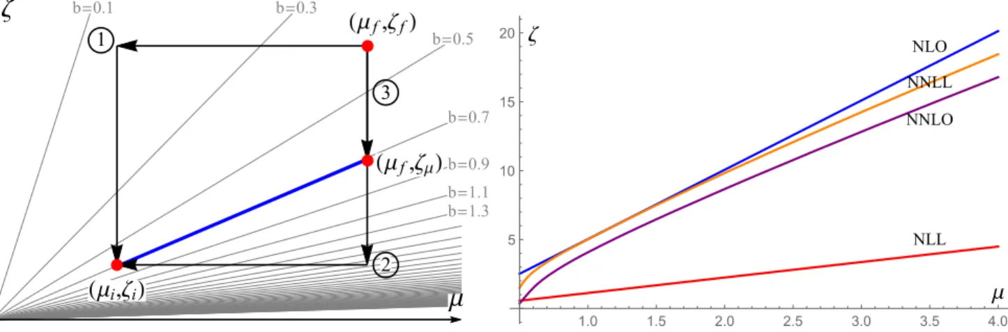
In a modern view, a TMD distribution is a cumbersome function of many factors, which mix up perturbative and non- perturbative information. In this context, the issue of the sep- aration of perturbative and non-perturbative physics requires a fine analysis and it is open to different solutions. The ζ - prescription proposed in this work, is an attempt to consider the perturbative input to a TMD distribution as it is, with- out artificial regulators. The ζ -prescription is founded on the fact that the TMD factorization introduces two factorization scales, one for the collinear and one for the soft exchanges.

These scales are usually fixed to the same point, while in the ζ -prescription they are chosen to eliminate the problematic double-log contributions. In other words, the ζ -prescription is based on the freedom to select the normalization and fac- torization scales, which is guaranteed by the structure of the perturbative theory. The ζ -prescription is essentially differ- ent from other used schemes. In particular, it does not strictly solve the problem of the large logarithmic contributions at large-b. It only decreases the power of the logarithmic con- tributions. However, the x-dependence of the remaining log- arithmic terms has a form which prevents the blow up of the perturbative series, which is not accidental, but the result of the charge conservation. In this way, the ζ -prescription post- pones the large logarithm problem to the very far domain of b-space, where other factors suppress a TMD distribution.

The practical implementation of the ζ -prescription shows that it is efficacious and it allows a very accurate and sound description of the data.

The description of the non-perturbative parts of TMD dis- tributions is the most interesting task. It is highly non-trivial because the definition of the non-perturbative part is strongly affected by schemes and prescriptions used in the perturba- tive implementation. In this respect a full NNLO can be clar- ifying. As an example, we recall that the non-perturbative behavior of the TMDPDFs is often assumed to have a Gaus- sian shape (see e.g. discussions in [15,22,24,25]). Although the Gaussian ansatz is widely used, it comes into conflict with the usual picture of long-distance strong interaction fueled by light-meson exchanges. The typically expected behav- ior at long distances is exponential, which is confirmed also by model calculations [26]. However, the Gaussian shape is often introduced together with the b ^∗ -prescription [27].

Notwithstanding many positive features, the b ^∗ -prescription has a serious issue: it introduces undesired b-even power cor- rections. In turn, these power correction introduced by b ^∗ can easily simulate the Gaussian behavior (see also discussion in [28]). Once the b ^∗ -prescription is removed the Gaussian ansatz for the TMD shape is no more essential, according to what we find.

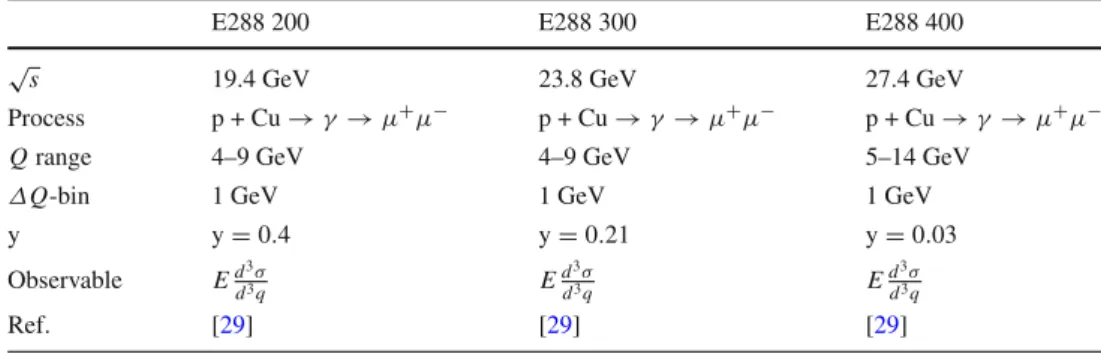
An additional remarkable point of the present study is the wide range of energies covered by the data that we have analyzed. The lowest energy measurements included in the fits have (Q, √

s) = (4, 19.4) GeV (E288 experiment [29]),

while the most energetic have (Q, √

s) = (116 − 150, 8 · 10 ³ ) GeV (ATLAS collaboration [30]). Typically, the low- and high-energy data are considered separately. The main reason for a separate scan is the assumed physical picture of strong interactions, which describes different energies. The description of the high-energy data requires a precise per- turbative input and it is expected to be less sensitive to the fine non-perturbative dynamics. The situation is the opposite for the low-energy measurements. Our experience shows that the inclusion of data of different energies is not only possi- ble within the TMD formalism, but it is also desired because it cuts away inappropriate models very sharply. We find also that the precision achieved by LHC is already sensitive enough to the non-perturbative structure of TMDs. We show that low and high energy data are sensitive to different regions of b-space, and consequently to different non-perturbative regimes of the TMDs: high energy data are better described by a Gaussian non-perturbative correction, while low energy data prefer an exponential type of non-perturbative models.

The code (arTemiDe) that we have prepared allows to test all these hypotheses, and can be adaptded also to test different non-perturbative inputs for TMDs.

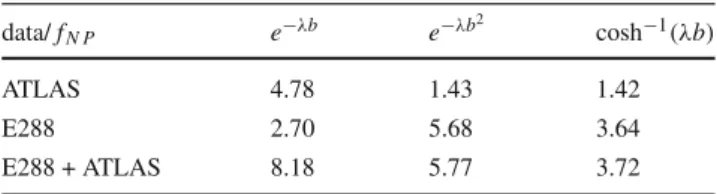
In order to extract the non-perturbative core of the TMDs, in the present study we choose a neutral tactic. We have scanned many possibilities such as a Gaussian and exponen- tial behavior, with/without inclusion of power corrections, and so on. We have also studied the non-perturbative cor- rection to the evolution kernel. During the examination of models we have prioritized the following criteria:

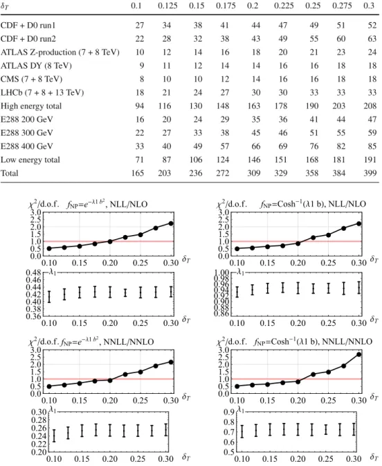
(i) Stability The TMD factorization is valid at small-q T

(the dilepton transverse momentum) up to a certain limit. Therefore, an acceptable model should produce a stable and good description within the allowed q T - range. In other words, the value of χ ² should be suffi- ciently close to one and the central values of the param- eters should be stable independently of the number of included data points (as far as the points belong to the allowed range).

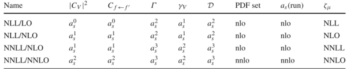
(ii) Convergence The agreement with data should improve with the increase of the perturbative order. Given the current state of the art of the theory, we can define four successive perturbative orders, which is enough to test the perturbative convergence. Also, the value of the phenomenological non-perturbative constants that one extracts should converge to some central value.

(iii) χ ² minimization Naturally, among the models with sim-

ilar behavior we select the model with the minimal χ ² .

We have found that it is difficult to find a model (with one

or two parameters), which fulfills the demands (i) and

(ii), and that at the same time provides a good χ ² value

on the whole set of data points (although it is relatively

easy to achieve this, selecting a particular experiment).

The models that we test consider a kind of minimal set of parameters which can be enlarged in future studies, refining the fitting hypotheses.

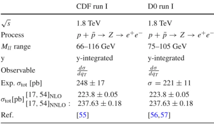
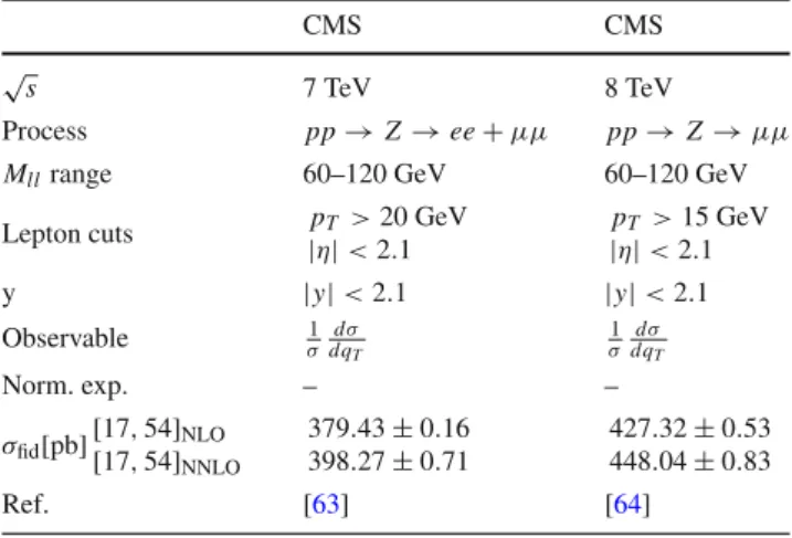
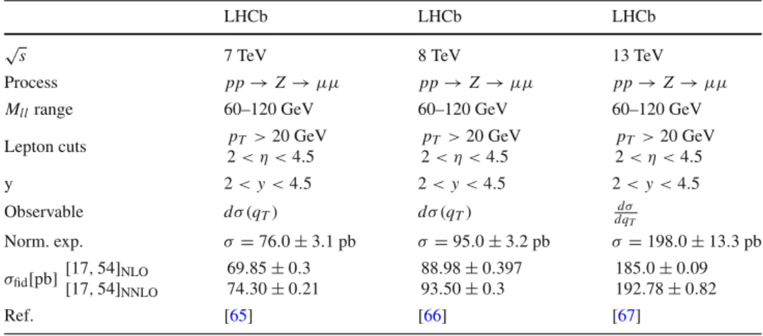
In the present fit, we have included the measurements of E288 at low-energies, Z-boson production at CDF, D0, ATLAS, CMS and LHCb, and Drell–Yan measurements from ATLAS.

To our knowledge, this is the largest set of Drell–Yan data points ever simultaneously considered in a fit within the TMD formalism. We find also that the LHC data below the Z-boson peak and at small q T are very important for current/future TMD studies. In the article we present the most successful models that we have found, and discuss some popular models.

In order to numerically evaluate the theoretical expres- sions, we have produced the package arTeMiDe.

arTeMiDe has a flexible module structure and can be used at any level of TMD theory description, from the evaluation of a single TMDPDF or evolution factor to an evaluation of differential cross-section. The arTeMiDe code is available at [31] and can be used to check our statements or test a possible future/alternative ansatz (for instance [14,32]). In arTeMiDe we have collected all recent achievements of TMD theory, including NNLO matching coefficient func- tion, and N ³ LO TMD anomalous dimensions. In the current version, arTeMiDe evaluates only unpolarized TMDPDFs and related cross-sections, however, we plan to extend it fur- ther.

The body of the article is divided as in the following. In Sect. 2 we review the theoretical construction of the Drell- Yan cross section and summarize the theoretical knowledge on unpolarized TMDPDFs. In this section, we also describe all the theoretical improvements which are original for this work. The main original point, namely ζ -prescription is pre- sented in Sect. 2.4 and “Appendix B”. The phenomenological studies are presented in Sect. 3. This section includes also a dedicated discussion of the shape of the non-perturbative part of the TMD. The allowed range of validity of the TMD factor- ization is explored in Sect. 3.4, the presentation of theoretical uncertainties is given in Sect. 3.5. The results of the final fit are presented in Sect. 3.7. A final discussion and conclusions can be found in Sect. 4.

2 Theoretical framework

We consider the Drell–Yan reaction h 1 + h 2 → G(→ ll ) + X, where G is the electroweak neutral gauge boson, γ ^∗ or Z . The incoming hadrons have momenta p 1 and p 2 with ( p 1 + p 2 ) ² = s. The gauge boson decays to the lepton pair with momenta k 1 and k 2 . The momentum of the gauge boson or equivalently the invariant mass of lepton pair is Q ² = q ² = ( k 1 + k 2 ) ² . The differential cross-section for the Drell–

Yan process can be written in the form [33,34]

d σ = d ⁴ q 2s

G , G

=γ, Z

L ^μν _GG

W _μν ^GG

Δ G (q )Δ G

(q ), (1) where 1/2s is the flux factor, Δ G is the (Feynman) propagator for the gauge boson G. The hadron and lepton tensors are respectively

W _μν ^GG

=

d ⁴ z ( 2 π) ⁴ e ^{− i q z}

× h 1 ( p 1 )h 2 (p 2 )|J _μ ^G (z)J _ν ^G

(0)|h 1 ( p 1 )h 2 (p 2 ), (2) L ^GG _μν

=

d ³ k 1

(2π) ³ 2 E 1

d ³ k 2

(2π) ³ 2 E 2 ( 2 π) ⁴ δ ⁴ ( k 1 + k 2 − q )

× l 1 (k 1 )l 2 (k 2 )|J _ν ^G (0)|00| J _μ ^G

(0)|l 1 (k 1 )l 2 (k 2 ), (3) where J _μ ^G is the electroweak current.

The point of our interest is the q T dependence of the cross-section, where q T is the transverse component of the produced gauge boson in the center-of-mass frame. More precisely, we are interested in the regime q T Q, where the TMD factorization formalism can be applied. Within the TMD factorization, one obtains the following expression for the unpolarized hadron tensor (see e.g. [35])

W _μν ^GG

= −g T μν

π N c

|C V (q, μ)| ²

f , f

z ^GG _{f f}

d ² b

4π e ^{i ( q b )}

× F f ← h

(x 1 , b; μ, ζ 1 )F f

← h

(x 2 , b; μ, ζ 2 )+Y μν , (4) where g T is the transverse part of the metric tensor and the summation runs over the active quark flavors. The variable μ is the hard factorization scale. The variables ζ 1 , 2 are the scales of soft-gluons factorization, and they fulfill the rela- tion ζ 1 ζ 2 Q ⁴ . In the following, we consider the symmetric point ζ 1 = ζ 2 = ζ = Q ² . The variables x 1 , 2 are the longitu- dinal parts of parton momenta

x 1 =

Q ² + q _T ²

√ s e ^y Q

√ s e ^y ,

x 2 =

Q ² + q _T ²

√ s e ^{− y} Q

√ s e ^{− y} . (5)

The factors z ^GG _{f f}

are the electro-weak charges and they are

given explicitly in Sect. 2.1. The factor C V is the match-

ing coefficient of the QCD neutral current to the same cur-

rent expressed in terms of collinear quark fields. The explicit

expressions for C V can be found in [36–38], and are also

given in “Appendix A”. The functions F f ← h are the unpolar-

ized TMDPDFs for quark f in the hadron h. They are uni-

versal non-perturbative functions and the main objects of our study. The details of their definition and their parametriza- tion are given in Sect. 2.3. Finally, the term Y denotes the power corrections to the TMD factorization theorem (to be distinguished from the power corrections to the TMD oper- ator product expansion). The Y -term is of the order q T /Q and composed of TMD distributions of the higher dynamical twist. In our study, we restrict ourself to the limit of low q T

such that the Y -term can be dropped.

Evaluating the lepton tensor, and combining together all factors one obtains the cross-section for the unpolarized Drell–Yan process at leading order of the TMD factoriza- tion, in the form [1,2,6,39–41]

d σ

d Q ² d yd ( q _T ² ) = 4π 3N c

P s Q ²

GG

z _ll ^GG

(q )

f f

z ^GG _{f f}

|C V (q , μ)| ²

× d ² b

4π e ^{i ( bq )} F f ← h

(x 1 , b; μ, ζ )

×F f

← h

(x 2 , b; μ, ζ ) + Y, (6) where y is the rapidity of the produced gauge boson. The factorP is a part of the lepton tensor and contains information on the fiducial cuts. It is discussed in details in Sect. 2.6. In the rest of this section a more detailed description of the particular components is presented.

2.1 Expressions for cross-section for different produced bosons

In the case of neutral vector bosons production, the sum over G and G in Eq. (6) has three terms

d σ

d Q ² d yd ( q _T ² ) = d σ ^{γ γ}

d Q ² d yd ( q _T ² ) + d σ ^{Z Z} d Q ² d yd ( q _T ² ) + d σ ^{γ Z}

d Q ² d yd ( q ² _T ) , (7) which correspond to γ ^∗ -production, Z -production and inter- ference of γ ^∗ -Z production amplitudes. These three terms of the cross-sections differ from each other only due to the factors z ^GG _{f f}

in Eq. (6), which are

z ^{γ γ} _ll

z ^{γ γ} _{f f}

= δ _{f f ¯} α ² _em (Q)e ² _f , z _ll ^{Z Z}

z ^{Z Z} _{f f}

= δ f f ¯ α ² em (Q)Q ⁴

(Q ² − M ² _Z ) ² + Γ _Z ² M _Z ²

1 − 4s ² _W + 8s _W ⁴ 8s _W ² c ² _W

× 1 − 4|e f |s _W ² + 8e ² _f s _W ⁴ 8s _W ² c ² _W

z _ll ^Z

^γ z ^Z _{f f} ^γ

+ z ^γ _ll

^Z z ^γ _{f f} ^Z

= δ _{f f ¯} α _em ² (Q)2 Q ² (Q ² −M _Z ² ) (Q ² − M ² _Z ) ² + Γ _Z ² M ² _Z

1 − 4s _W ² 4s W c W

× |e f |(1 − 4|e f |s ² _W )

4s W c W , (8)

where M Z and Γ Z are the mass and the width of the Z-boson, s W and c W are sine and cosine of the Weinberg angle. We use the following of values [42]

M Z = 91.2 GeV, Γ Z = 2.5 GeV, s _W ² = 0.2313. (9) In many studies (see e.g.[15,19,20,22,43]) the contribution of γ ^∗ to the cross-section is neglected in the vicinity of the Z- peak, i.e. the zero-width approximation is used. Here, instead, we include the γ ^∗ and interference terms in the evaluation of the the cross-section. The inclusion of these terms is impor- tant for LHC (in particular ATLAS experiment), where the measurement precision often exceeds the theory precision.

2.2 TMD parton distributions: evolution

The quark unpolarized TMDPDFs are given by the matrix element [1,2,11]

F

( x , b ;ζ, μ)

= Z

(ζ, μ)R

(ζ, μ) 2

X

d ξ

2 π e

×

h|

T

q ¯

W ˜

a

ξ 2

|X

γ

X| ¯ T W ˜

q

a

−ξ 2

|h

, (10) where n is the light-cone vector along the large component of the hadron momentum, ξ = {0 ⁺ , ξ ⁻ , b}, Z and R are the ultraviolet and rapidity divergence renormalization factors.

The Wilson lines W n pointing along the direction n to the infinity. For the detailed definition of all constituents in this expression we refer to [11].

The peculiar feature of the TMD operator is the pres- ence of two types of divergences and, as a consequence, two renormalization factors Z and R. Firstly, we have ultra- violet divergences, which have their collinear counterpart in the coefficient function C V . These divergences are the result of collinear factorization and give rise to the loga- rithms of the factorization scale μ. Secondly, we have rapid- ity divergences, which arise in the factorization of the soft- gluon exchanges between partons. The singular soft-gluons exchanges can be collected into the soft factor, which in turn, can be written as a product of rapidity renormalization fac- tors R, see e.g. [10,11,44]. This procedure introduces the rapidity factorization scale ζ .

The dependence of TMDPDF on the factorization scales μ and ζ is given by the pair of evolution equations

μ ² d

dμ ² F f ← h (x, b; μ, ζ ) = 1

2 γ _F ^f (μ, ζ )F f ← h (x, b; μ, ζ ), (11) ζ d

d ζ F f ← h (x, b; μ, ζ ) = −D ^f (μ, b)F f ← h (x, b; μ, ζ ).

(12)

The TMD anomalous dimensions γ and D are known up to order a _s ³ (see [45] for γ V , and [44,46,47] for D ). They sat- isfy the consistency condition (Cauchy–Riemann condition), which guaranties the existence of the common solution for equations (11) and (12),

ζ d dζ

γ _F ^f (μ, ζ )

2 = μ ² d

dμ ² (−D ^f (μ, b)) = − Γ ^f (μ) 2 , (13) where Γ ^f is the cusp anomalous dimension. This equation fixes the logarithmic part of the anomalous dimensions. So, the anomalous dimensionγ is linear in logarithm at all orders, while the rapidity anomalous dimension D has all powers of logarithms,

γ _F ^f = Γ ^f l _ζ − γ _V ^f , D ^f = ∞ n = 1

a _s ⁿ n k = 0

L ^k _μ d ⁽ _f ^{n , k )} . (14) Here and in the following, we use the following notation for logarithms

L X = ln

b ² X 4e ^{− 2 γ}

, l X = ln μ ²

X . (15)

The explicit expressions for the anomalous dimensions up to third-loop order can be found e.g. in the “Appendix” of [11,44].

The initial values of the factorization scales are dictated by the kinematics of the considered process. In particular, the scales ζ 1 , 2 are related to the momentum of hard partons as ζ 1 ζ 2 = ( 2 p ⁺ ₁ p ⁻ ₂ ) ² = ( Q ² + q ² _T ) ² Q ⁴ . (16) In the following, we use the symmetric normalization point, ζ 1 = ζ 2 = ζ = Q ² . The μ -dependence cancels between the parts of factorization formula, namely between hard coeffi- cient function |C V | ² and the TMDPDFs. The natural choice of μ is such that logarithms appearing in | C V | ² are mini- mized, i.e. μ = Q. Therefore, TMDPDFs enter in the cross- section in Eq. (6) at the hard point (μ f , ζ f ) = (Q, Q ² ).

A typical construction of a model for a TMD distribution requires its evolution to a different set of scales. The evolution from (μ f , ζ f ) to (μ i , ζ i ) takes the form

F f ← h (x, b; μ f , ζ f ) = R ^f [b; (μ f , ζ f ) → (μ i , ζ i )]

×F f ← h (x, b; μ i , ζ i ), (17) where

R ^f [b; (μ f , ζ f ) → (μ i , ζ i )]

= exp

P

γ _F ^f (μ, ζ ) d μ

μ − D ^f (μ, b) d ζ ζ

. (18)

Here, the

P denotes the integration along the path P in the (μ, ζ )-plane from the point (μ f , ζ f ) to the point (μ i , ζ i ).

The integration can be done on an arbitrary path P, and the solution is independent of it, thanks to the Cauchy–Riemann

condition Eq. (13). At a finite perturbative order, the con- dition Eq. (13) is violated by the next perturbative order.

As a consequence the expression for the evolution factor R is dependent on the path of integration. The two simplest choices of integration paths are the combinations of straight segments as

path 1 : (μ f , ζ f ) → (μ i , ζ f ) → (μ i , ζ i ), path 2 : (μ f , ζ f ) → (μ f , ζ i ) → (μ i , ζ i ).

These paths are depicted in Fig. 1. The factor R evaluated along these paths reads

R ^f [ b ; (μ f , ζ f ) − → ¹ (μ i , ζ i )]

= exp _μ

μ

d μ

μ γ _F ^f (μ, ζ f ) − D ^f (μ i , b) ln ζ f

ζ i

,

(19) R ^f [b; (μ f , ζ f ) − → ² (μ i , ζ i )]

= exp _μ

μ

d μ

μ γ _F ^f (μ, ζ i ) − D ^f (μ f , b ) ln ζ f

ζ i

.

(20) The numerical difference between these two expressions rep- resents the value of the uncertainty at a given perturbative order.

The expressions for the evolution factor R given in Eqs. (19) and (20), contain the rapidity anomalous dimension D(μ, b). The latter contains potentially large values of L _μ , which should be resummed with the help of Eq. (13). Addi- tionally, the rapidity anomalous dimension can acquire power corrections from the higher orders in the power expansion of the factorization theorem [48]. These power corrections can be also observed in the renormalon structure described in [12]. The non-perturbative correction takes the form of a series of even powers of the transverse distance. Therefore, the practical expression for the rapidity anomalous D is D ^f (μ, b) =

_μ

μ

d μ

μ Γ ^f + D _pert ^f (μ 0 , b) + g K b ² , (21) where g K is an unknown parameter. Here, D pert ^f is the per- turbative expression for D. Correspondingly, the value μ 0

should be chosen such that L _μ

is minimal in the pertur- bative region. Substituting this expression to the evolution factor, we obtain

R ^f [b; (μ f , ζ f ) → (μ i , ζ i ); μ 0 ]

= exp _μ

μ

d μ

μ γ _F ^f (μ, ζ f ) − _μ

μ

dμ

μ Γ ^f (μ) ln ζ f

ζ i

× ζ f

ζ i

_−D

_(μ

_, b )− g

b

. (22)

In this form, the evolution factor R does not depend on the

path of evolution, as can be checked explicitly. The pertur-

Fig. 1 (left) The evolution plane (μ, ζ ) and paths for the evolution integrals from (μ

, ζ

) to (μ

, ζ

) . Gray lines are equi-evolution lines ζ

at different b. Paths 1 and 2 reprent the solutions in Eqs. (19) and (20), corespondingly. These solutions are equivalent to the evolution to the

point (μ

, ζ

) , which is shown by path 3, because there is no evolution along the blue segment (at b = 0 . 7 GeV

). (right) The plot of ζ

at b = 1 GeV

for different orders

Fig. 2 Schematic picture of the regions in b-space of the TMDPDF and the corresponding/needed theoretical treatment

bative uncertainty which previously has been given by the variation of evolution path, now is represented by the depen- dence on the parameter μ 0 . Thus, using Eq. (22) the uncer- tainties of the perturbative calculation can be measured by varying the scale μ 0 . In the following, we use the evolution factor as in Eq. (22).

2.3 TMD parton distributions: b-space behavior

The TMDPDF is a genuine non-perturbative function, which is to be fitted by a certain ansatz, which covers the whole domain in b-space. Different intervals of b-space describe different regimes of strong interactions. In Fig. 2 we show schematically the parts of b-space which need a specific treat- ment for each TMDPDF. In order to construct an optimal and physically meaningful fitting ansatz, the behavior in every part of the b-space should be reproduced. In this section, we collect the main information on the b-dependence of TMD-

PDFs, as it is understood according to the current state of art.

The starting point of our description of a TMD distribu- tion is the small-b operator product expansion (OPE), which results in the series

F q ← h (x, b; μ, ζ )

= ∞ n = 0

b ² B ²

n

f

C _q ^{( n} _← ⁾ _f ( b ; μ, ζ ) ⊗ f ⁽ _f ⁿ _← ⁾ _h (μ) ( x ),

(23) where f ^{( n )} are PDFs of a 2(n + 1)-twist, C ^{( n )} are coefficient functions of OPE and the symbol ⊗ represents the convolu- tion in momentum fractions of partons. The parameter B is an unknown non-perturbative parameter which represents an intrinsic hadron scale.

Region 1 In the range b B, the TMDPDF is dominated by the n = 0 term of OPE, Eq. (23). The leading term is represented by the usual matching onto twist-2 PDFs and reads

b B : F q ← h (x, b; μ, ζ )

=

f

₁

x

d z

z C q ← f (z, L _μ ; μ, ζ ) f f ← h

x z , μ

, (24)

where C is known up to two-loop order [11,49].

There is a subregion b 1/Q, which should be consid-

ered specially. While the TMD distribution is completely per-

turbative within this region, the contributions of this region to

the cross-section strongly overlaps with the Y -term, Eq. (4),

which is formally O(1/(b Q)). The behavior of TMD dis-

tributions within this tiny range together with the Y-term

dictates the asymptotics of the cross-section at large q T . As

a consequence, it has a significant influence on the value of the total cross-section. In our current evaluation we restrict ourself to the range of small-q T (for a dedicated study of the applicability of this approximation in practice, see Sect. 3.4).

Therefore, we drop the Y -term and do not need any special treatment of b Q ^{− 1} region.

Region 2 In the range b B the OPE is still valid. How- ever, one has to include the higher order terms in addition to the leading one. Very little is known about power suppressed terms of the small-b OPE. Our recent study of the renormalon singularities [12] suggests several hints that can be used to model this region:

(i) The OPE contains only even powers of b. Moreover, the coefficient function of n’th order has a prefactor x ⁿ . In other word, the natural scale of OPE is x b ² / B ² rather then just b ² /B ² .

(ii) The higher order OPE contributions induced by renor- malons, can be summed together to some effective non- perturbative function under the convolution integral.

Therefore, in this region the TMDPDF can be approximated by the form

b ∼ B : F q ← h ( x , b ; μ, ζ )

=

f

₁

x

d z z G q ← f

z, zb ²

B ² , L _μ ; μ, ζ

× f f ← h

x z , μ

, (25)

where the leading term of the power series in b/B of G is given by C. As the power n grows, the sub-leading terms of OPE switch on, which is schematically presented by gray lines in Fig. 2. The particular contributions at higher n are not so important in the continuous TMD picture. However,

(iii) The n = 1 contribution to OPE can be estimated by the leading renormalon contribution of order ∼ x b ² [12].

It has the form

C _q ^ren _{← q} (x, b; μ, ζ ) = 2 x ¯ + 2x ( 1 − x ) +

− δ( x) ¯ L _Λ − L ^√ _ζ + 2 3

, (26)

where Λ = Λ QC D is the position of the Landau pole.

Region 3 At b B the small-b OPE cannot be consid- ered as a source of information, and the TMD is completely non-perturbative. Luckily, this region is suppressed by the evolution factor. As a consequence, the cross-section is not very sensitive to the fine structure of TMD distribution in this region, but the general behavior is important. We have

tested several asymptotical forms of the TMDPDF, including Gaussian, exponential and power-like and found that the best agreement with the experimental data is achieved with expo- nential behavior. This observation is in agreement with the general physical intuition, that at high distances the strong forces are dominated by meson exchange, while the Gaus- sian and power-like asymptotics can not be produced in any simple way.

We should mention that the size of the parameter B, as well as, the order of convergence of the small-b OPE, which influ- ences the size of the intermediate region 2, are not known.

Our estimations of these characteristic sizes are presented in Sect. 4.

2.4 Definition of scaling parameters

The small-b matching is the starting point for the construction of the majority of phenomenological ansatzes for TMD distri- butions. It can be considered as an additional collinear factor- ization, which is performed at some convenient set of scales (μ i , ζ i ). The difference of (μ i , ζ i ) from the initial (defined by process kinematic) scales of TMD distribution is compen- sated by the evolution factor in Eq. (17). As usual, the all- order expression is independent of (μ i , ζ i ), but in practice, these scales are to be chosen such that the coefficient function C f ← f

has good perturbative convergence. This procedure is alike the choice of hard-factorization scale, with one essen- tial difference: the parameter b, which accompanies μ i and ζ i in the logarithms, has no fixed value. It varies from zero to infinity within the Fourier integral.

The choice of scales (μ i , ζ i ) is one of the central point of the TMD phenomenology. To make the discussion clearer, let us recall the expression for the coefficient function at NLO.

It reads

C q ← q (x, L _μ ; μ, ζ )

= δ( x ¯ ) + a s (μ) C F

− 2L _μ 2

(1 − x) ₊ − 1 − x

+ 2 x ¯ + δ( x) ¯ −L ² _μ + 2L _μ l _ζ − π ² 6

, (27)

where the notation for the logarithms is defined in Eq. (15).

Ideally, the scales μ and ζ should be chosen such that no large perturbative contributions appear in the coefficient function.

Clearly, it cannot be done at arbitrary b due to the presence of

μ in the coupling constant and in L _μ . However, such a strict

choice is not required. The only requirement for scales is to

keep the perturbative ansatz stable, i.e. to prevent its blow-

ing up. There are several solutions of this problem. The most

famous is the b ^∗ -prescription [27]. Within the b ^∗ -prescription

the logarithms L _μ are absent, and this fact allows the con-

trol of the perturbative series in the full region of b. How-

ever, the b ^∗ -prescription introduces artificial power correc-

tions to the small-b OPE, which washes out any theoretical intuition. Another popular scheme [50,51] is based on the re- expression of Hankel-integral as an integral in the complex b-plane. In this way, the logarithms L _μ can be minimized by μ ∼ b ^{− 1} and the Landau pole at large-b is by-passed in the complex plane. The drawback of this scheme is the neces- sity of the analytical continuation into the complex b-plane, and the restriction to NNLO (since the analytical solution for running coupling at N ³ LO is unknown).

In this work we use another scheme which we call ζ - prescription. It is a novel one (to our best knowledge), and it is described in the following.

The ζ -prescription uses the fact that the TMD operator and hence its small-b OPE depends on two scales μ and ζ , which are entirely independent. This simple fact has been overlooked so far. Indeed, the first typical step is to fix ζ = C ₀ ² /b ² , or ζ = μ ² [1,12,52]. It reduces the problem to a single variable problem, which looks simpler, but finally, it does not provide a simple solution for the appearance of large logarithms in the OPE.

The initial point of the ζ -prescription is the observation that not all logarithms in the coefficient function are danger- ous. So, the terms L ² _μ and L _μ l _ζ in Eq. (27) are problematic, while the logarithm in the first term is not. There are several reasons for it. First, the double logarithm contributions vio- late the normal perturbative counting and at large-b grows faster than the single logarithms. Second, the first term of Eq. (27) comes together with the DGLAP kernel, and thus, it preserves the area (say, the integral over x) of the TMD- PDF, due to the conservation of the electromagnetic charge.

We remind that logarithms accompanying the DGLAP ker- nel are related to PDF evolution, while the rest of logarithms are related to the TMD evolution. For this reason, the main problem of convergence is represented by the logarithms that are related to the TMD evolution. The logarithms related to the PDF evolution come with a particular x-dependent func- tion. The probabilistic interpretation of PDF ensures their minimal contribution in the very large domain of b. Practi- cally, this fact has been already demonstrated although not entirely realized in the fit [20]. In the realization of Ref. [20], the DGLAP logarithms were left unregulated and they do not influence the convergence of the fit.

The logarithms related to the TMD evolution can be elim- inated completely by a particular choice of ζ = ζ _μ . Along the curve ζ μ , the TMD distributions are independent of μ. In other words, the curve ζ _μ is an equi-evolution curve in the plane (μ, ζ ). Such a curve satisfies the equation

μ ² d F(x, b; μ, ζ _μ )

d μ ² = 0. (28)

Using the definition of anomalous dimensions in Eq. (11) we rewrite this equation as

D(L _μ ) f (L _μ ) + Γ

2 f (L _μ ) − D(L _μ ) − γ V

2 = 0, (29)

where f (L _μ ) = l _ζ

. The perturbative solution is discussed and presented in the “Appendix B.1”. The curve ζ μ is dif- ferent for quark and for gluon TMDs, and it is expressed in terms of the TMD anomalous dimensions Eq. (62). In our analysis, we need only the quark case. Up to NNLO it reads l _ζ

= L _μ

2 − 3 2 + a s

11C A − 4T F N f

36 L ² _μ + C F − 3

4 + π ² − 12ζ 3

+ C A

649

108 − 17π ² 12 + 19

2 ζ 3

+ T F N f − 53 27 + π ²

3

+ O(a ² s ). (30) Note, that in Eq. (30) we have set the boundary condition such that no terms singular at L _μ → 0 appear in l _ζ (see “Appendix B.1”, for details). Also, in the current work we drop the power contributions to the rapidity anomalous dimension D. The influence of these decisions should be investigated later. One can check that the leading term of ζ _μ (i.e. l _ζ = L _μ /2) cancels leading powers of logarithms at all orders in perturbation the- ory (i.e. all terms a ⁿ _s L ²ⁿ _μ ). Then, including the next correction (a s β 0 L ² _μ /12) cancels subleading powers of logarithms at all orders of the perturbation theory (i.e. all terms a _s ⁿ L ²ⁿ _μ ^{− 1} ) , and so on.

Substituting the leading term of the solution in Eq. (30) to the quark small-b coefficient function, we obtain

C q ← q (x, L _μ ; μ, ζ _μ )

= δ( x) ¯ + a s (μ)C F

−2L _μ 2

(1 − x) ₊ − 1 − x

+ 2 x ¯ + δ( x) ¯ −3L _μ − π ² 6

. (31)

This coefficient function is stable for any value of L _μ , which can be seen by considering its integral

1 0

d xC q ← q (x, L _μ ; μ, ζ _μ ) = 1 + a s (μ)C F 1 − π ² 6

, (32) which is independent of L _μ .

The general expression for the coefficient of arbitrary flavour at NNLO has the form

C f ← f

(x, b; μ, ζ _μ )

= δ f f

δ( x) ¯ + a s

−L _μ P ⁽ _f ¹ _← ⁾ _f

+ C ⁽ _f ¹ _← ^{, 0 )} _f

+ a _s ²

⎡

⎣L ² _μ P ⁽ _f ¹ _← ⁾ _k ⊗ P _k ⁽ _← ^{1 )} _f

− β 0 P ⁽ _f ¹ _← ⁾ _f

2

− L _μ

P ⁽ _f ² _← ⁾ _f

+ C ⁽ _f ¹ _← ^{, 0 )} _k ⊗ P _k ⁽ _← ^{1 )} _f

− β 0 C ⁽ _f ¹ _← ^{, 0 )} _f

+ d ⁽ _f ^{2 , 0 )} γ _V ^{f ( 1 )}

Γ ₀ ^f δ( x) ¯ + C ⁽ _f ² _← ^{, 0 )} _f

⎤

⎦ + O(a ³ _s ), (33)

where C ^{( n , 0 )} is the finite part of the coefficient function at n’th perturbative order, and P(x) =

a _s ⁿ P ^{( n )} is the DGLAP kernel. The detailed derivation of Eq. (33) is presented in the

“Appendix B.2”. Eq. (33) has the form of the usual coefficient function for an object without external evolution (e.g. coeffi- cient function for DIS). In other words, it is straightforward to check that

μ ² d

d μ ² C f ← f

(x, b; μ, ζ _μ ) ⊗ f f

← h (x, μ) = 0, (34) by direct differentiation of Eq. (33). The integral of this func- tion over x is independent of L _μ due to the charge conserva- tion, and thus at least the area of TMDPDF is stable at large b.

A further positive point of the ζ -prescription is that the scale μ remains unconstrained. Often, the scale μ is selected such that it behaves as ∼ 1/b at b → 0. Such a choice minimizes the small-b logarithms in small-b OPE and in the evolution exponent. At large-b the scale μ should be frozen to some fixed value (of the order of a few GeV’s), in order to avoid the Landau pole. We use the simplest function which satisfies these criteria

μ = μ b = C 0

b + 2 GeV. (35)

There are several practical motiviations for the choice of the 2 GeV asymptotic (at b → ∞) scale. To start with, the fixed scale 2 GeV is a standard scale of PDF extractions. The data that we analyze start with a dilepton invariant mass of 4 GeV, so that we want to fix the starting scale below this energy. On the other side we do not want to implement a perturbative expansion below 1 GeV, where the convergence of the the- ory is not ensured. A discussion about the theoretical error induced by this choice in the interval 1–4 GeV is posponed to Eq. (37).

Finally, we should also select the value for the parame- ter μ 0 that enters in the expression for the evolution factor, Eq. (22). To keep our discussion simple, we set μ 0 = μ b . 2.5 Theoretical uncertainties and perturbative ordering In the construction of the cross section, one finds several sources of perturbative uncertainties. The size of these uncer- tanties can be estimated by the variation of associated scales.

We list here the ones that we have considered in the present work.

– Uncertainty associated with the perturbative matching of rapidity anomalous dimension This uncertainty arises from the dependence (at the fixed perturbative order) on μ 0 , which should be compensated between the Sudakov factor and the boundary term D(μ 0 ) in the TMD evo- lution factor Eq. (22). This uncertainty can be tested by changing μ 0 → c 1 μ 0 and varying c 1 ∈ [0.5, 2].

– Uncertainty associated with the hard factorization scale This uncertainty arises from the dependence (at the fixed perturbative order) on the scale μ f (∼ Q) which is to be compensated between the hard coefficient function

|C V | ² and the TMD evolution factor. This uncertainty can be tested by changing μ f → c 2 μ f and varying c 2 ∈ [ 0 . 5 , 2 ] .

– Uncertainty associated with the TMD evolution fac- tor This uncertainty arises from the dependence (at the fixed perturbative order) on the initial scale of TMD evolution μ i , which is to be compensated between the evolution integral and the μ-dependence of ζ i in Eq. (22).

This uncertainty can be tested by changing μ i → c 3 μ i

and varying c 3 ∈ [0.5, 2].

– Uncertainty associated with the small-b matching This uncertainty arises from the dependence (at the fixed per- turbative order) on the scale of the small-b matching μ OPE which is to be compensated between the small- b coefficient function C _{f ← f} and evolution of PDF. This uncertainty can be tested by changing μ OPE → c 4 μ OPE

and varying c 4 ∈ [0.5, 2].

We remark that our definition of perturbative uncertain- ties c 1 , 2 is commonly used in the literature (as far as it can be compared among different schemes of calculation), see e.g. [21,43]. Usually the uncertainties c 3 , 4 are not distin- guished and they are commonly varied simultaneously i.e.

in the literature one finds discussions of errors for the case c 4 = c 3 . To our best knowledge, the distinction of the match- ing and evolution uncertainties is made here for the first time.

In this way, the general expression for the cross-section in Eq. (6) with our choice of scales reads

d σ d Q ² d yd(q _T ² )

= 4 π 3 N c

P s Q ²

GG

z _ll ^GG

(q )

×

f f

z ^GG _{f f}

d ² b

4π e ^{i ( bq )} |C V (Q, c 2 Q)| ²

×

R ^f [b; (c 2 Q, Q ² ) → (c 3 μ i , ζ c

μ

); c 1 μ i ] 2

Table 1 The perturbative orders studied in the fit. For each order we indicate the power of a

of each piece that enters in the TMDs. Note, that the order of a

and PDF set are related, since the values of a

are taken from the PDF set

Name | C

|

C

Γ γ

D PDF set a

(run) ζ

NLL/LO a

a

a

a

a

nlo nlo NLL

NLL/NLO a

a

a

a

a

nlo nlo NLO

NNLL/NLO a

a

a

a

a

nlo nlo NNLL

NNLL/NNLO a

a

a

a

a

nnlo nnlo NNLO

× F f ← h

(x, b; c 4 μ OPE , ζ c

μ

)F f

← h

× (x, b; c 4 μ OPE , ζ c

μ

), (36) where the evolution factor R is given in Eq. (22) and the explicit expression for the ζ _μ is given in Eq. (30). The low- normalization point μ i and the scale of small-b operator prod- uct expansion μ OPE are fixed at the same point as in Eq. (35) μ i = μ OPE = C 0

b + 2 GeV . (37)

In the limit b → ∞ the scale μ i reaches the fixed point of 2 GeV, cfr. Eq. (35). The error induced by this choice of the asymptotic energy scale is evaluated together with the error induced by the scale μ i . In particular, one observes that the variation of c 1 , 3 , 4 in formula (36) allows to test the impact of the variation of the fixed scale of 2 GeV in the whole range 1–4 GeV, as discussed around Eq. (35).

The perturbative orders of each cross section constituent are to be combined consistently. Having at our disposal the NNLO expressions for coefficient function and N ³ LO expressions for anomalous dimensions, we can define four successive self-contained sets of ordering. This is reported in Table 1. In our definition of orders we use the following logic: (i) The order of the a s -running should be the same as the order of PDF set, since their extraction are correlated. (ii) The order of D should be the same as the order of Γ since they enter the evolution kernel R with the same counting of logarithms (i.e. a _s ⁿ ln ^{n + 1} μ ), and one-order higher then the order of γ V , since it has counting a ⁿ _s ln ⁿ μ. (iii) The order of small-b matching coefficient should be the same as the order of evolution of a PDF, because large logarithms of b are to be compensated by the PDF evolution. (iv) The order of ζ _μ should be such that no logarithms appear in the coefficient function, and the general logarithm counting coincides with the counting of the evolution factor. In Table 1 the order of the ζ _μ is defined as following: NLL is l _ζ = L _μ /2, NLO has in addition finite part at order a _s ⁰ (i.e. two first terms of Eq. (30)), NNLL has in addition logarithmic part at order a _s ¹ (i.e. the first line of Eq. (30)), and NNLO is given by whole expres- sion Eq. (30). The l _ζ cases NLL and NNLL are somewhat intermediate cases. In fact, while one achieves a cancella- tion of logs of the same order in the evolution kernel and the coefficient, one finds that the counting in the coefficient is consistent with the a s L ² _μ ∼ a _s ⁰ . A similar counting was

introduced in [53]. We postpone a full study of this counting within ζ -prescription to a future work.

To label the orders we use the nomenclature where the part with ’LO suffix designates the order of coefficient functions, and the part with ’LL suffix designates the order of the evo- lution factor in the a s ln μ ∼ 1 scheme. So, our highest order is NNLL/NNLO, which at the moment the highest available combination of the perturbative series. The order NLL/LO appears to be barely inconsistent, because it requires the LO PDF evolution to match the trivial coefficient function.

Therefore, we exclude the NLL/LO from our phenomeno- logical studies.

2.6 Implementation of lepton cuts

In modern experiments, the cross-section is often evaluated using fiducial cuts on the dilepton momenta. That is, the lep- ton tensor in Eq. (3) should be evaluated taking into account the experimental cut phase-space. At leading order the lepton tensor takes the form

(− g ^μν _T ) L _μν ^GG

= 32z ^GG _ll

d ³ k 1

2E 1

d ³ k 2

2 E 2 (( k 1 · k 2 )

+ (k 1 · k 2 ))θ(k 1 , 2 ∈ cuts)δ ⁴ (k 1 + k 2 − q), (38) where θ-function restricts the lepton momenta to the allowed region.

In the limit Q → ∞ and no restriction on the lepton pair phase space we obtain

Q lim →∞ (−g ^μν _T )L _μν ^GG

= 16π

3 z ^GG _ll

Q ² . (39)

Substituting this expression to the cross-section we obtain the standard formula to the Drell-Yan cross-section within TMD factorization [1,2,6,39–41]. In order to include the corrections due to a finite Q and experimental cuts let us introduce a factor P , i.e.

(− g ^μν _T ) L _μν ^GG

= 16π

3 z ^GG _ll

Q ² P , (40)

which is consistent with the cross section expression pre- sented in Eq. (6). The function P in the absence of cuts reads P (no cuts) = 1 + q _T ²

2 Q ² . (41)