Unitarity violation in noninteger dimensional Gross-Neveu-Yukawa model

(1)

Unitarity violation in noninteger dimensional Gross-Neveu-Yukawa model

Yao Ji

^*

and Michael Kelly

^†

Institut für Theoretische Physik, Universität Regensburg, D-93040 Regensburg, Germany

(Received 24 February 2018; published 3 May 2018)

We construct an explicit example of unitarity violation in fermionic quantum field theories in noninteger dimensions. We study the two-point correlation function of four-fermion operators. We compute the one- loop anomalous dimensions of these operators in the Gross-Neveu-Yukawa model. We find that at one-loop order, the four-fermion operators split into three classes with one class having negative norms. This implies that the theory violates unitarity, following the definition in Ref. [1].

DOI:10.1103/PhysRevD.97.105004

I. INTRODUCTION

Conformal field theories (CFTs) have always been an area of active research due to their rich mathematical structure and physical applications. In unitary theories conformal symmetry imposes severe constraints on the spectrum of operator dimensions. It is believed that these dimensions can be determined with the help of the conformal bootstrap technique [2,3]. This technique has proved to be extremely useful for solving two-dimensional CFTs. The effective numerical algorithms for solving the bootstrap equations for higher-dimensional CFTs have been proposed in Ref. [4] (see also Refs. [5 – 7], [8 – 13], and [14 – 18] for more details and recent developments in d ¼ 3 , d ¼ 4 , and d ¼ 5 dimensions, respectively). One of the advantages of this approach is that it allows one to obtain operator dimensions directly in various integer dimensions.

The standard technique for the calculation of the operator dimensions, the so-called ϵ -expansion [19,20], is based on calculation of the scaling dimensions in d ¼ 4 − 2ϵ dimen- sional theory and interpolation of the relevant critical indices to the physical dimension. The critical indices for many CFTs are known with high precision. One of the recent achievements is the calculation of the six-loop β function in the φ

⁴

theory [21]. In order to get a better understanding of the new conformal bootstrap technique it was quite natural to apply it to theories in noninteger dimensions, d ¼ 4 − 2ϵ (see Refs. [22,23]). At the same time, one of the assumptions which most of the conformal

bootstrap relies on is the unitarity of the theory. One can hardly expect that this assumption — unitarity — will be true for theories in noninteger dimensions. This question was raised in Refs. [1,24], where unitarity violation in φ

⁴

theory was demonstrated by constructing states (operators) with negative norm. The first “ negative norm ” operator in φ

⁴

theory has a rather high scaling dimension ( Δ ¼ 23 ), and it is expected that unitarity breaking effects will appear only in high orders of ϵ expansion. Negative norm operators necessarily have to be evanescent operators, i.e., operators that are vanishing in integer dimensions. In scalar theories the building blocks for the operators are fields, and their derivatives and therefore evanescent operators are must have a high dimension. The situation is quite different in theories with fermions where there are evanescent (scalar) operators of canonical dimension six [25].

The aim of this article is to demonstrate the existence of the negative norm states in the d ¼ 4 − 2ϵ dimensional Gross—Neveu—Yukawa (GNY) model [26]. It was argued in [1] that unitarity implies the positiveness of the coef- ficient C in the correlator

hO

^†

ðxÞOð0Þi ¼ C=x

^2Δ

; ð1Þ where O is a conformal operator with scaling dimension Δ . In an integer dimensional CFT, violation of this condition indicates the presence of negative norm states in the theory [1]. We consider the renormalization of an infinite set of scalar four-fermion operators in d ¼ 4 − 2ϵ dimensions and show that the positiveness condition is broken for infinitely many operators. Since the canonical dimension of these operators is not large, Δ

^can

¼ 6 , one can wonder about the effect of negative norm operators to the conformal bootstrap technique.

The article is organized as follows: In Sec. II we discuss the two-point correlation function of scalar four-fermion operators in free theory. We find that the theory contains

*

yao.ji@ur.de

†

Michael.Kelly@stud.uni-regensburg.de

Published by the American Physical Society under the terms of the Creative Commons Attribution 4.0 International license.

Further distribution of this work must maintain attribution to

the author(s) and the published article ’ s title, journal citation,

and DOI. Funded by SCOAP

³

.

(2)

evanescent operators which could generate negative norm states.

In order to continue our discussion, we then compute in Sec. III the anomalous dimension of the physical and evanescent operators at one-loop order in the GNY model.

It turns out that all the evanescent operators split into two classes of definite anomalous dimension. We show that the negative norm states are generated by one of these two classes, depending on the number of fermion flavors of the theory.

II. FOUR-FERMION CORRELATION FUNCTION IN NONINTEGER DIMENSIONS

The GNY model describes an interacting fermion-boson system with the Lagrangian given by the following expression [26,27]:

L ¼ 1

2 ð∂

μ

σÞ

²

þ Ψ ¯

i

∂ Ψ

i

þ g

₁

σ Ψ ¯

i

Ψ

i

þ 1

24 g

₂

σ

⁴

; ð2Þ where the index i ¼ 1 ; … ; n

_f

enumerates different fermion flavors and σ is a scalar field.

The model has an infrared stable fixed point in d ¼ 4 − 2ϵ dimensions [28]. At one loop the critical couplings take the form

u

¼ ðg

₁

Þ

²

ð4πÞ

²

¼ ϵ

N

_f

þ 6 ; v

¼ ðg

₂

Þ

²

ð4πÞ

²

¼ 6 − N

_f

þ ffiffiffiffiffiffiffiffiffiffiffiffiffiffiffiffiffiffiffiffiffiffiffiffiffiffiffiffiffiffiffiffiffiffiffiffi N

²_f

þ 132 N

_f

þ 36 q

6ðN

f

þ 6Þ ϵ ; ð3Þ where N

_f

≡ n

_f

trðI

d

Þ. The basic critical indices are now known with four-loop accuracy and can be found in Ref. [29].

Let us consider an infinite system of four-fermion local operators in d ¼ 4 − 2ϵ dimensions

O

^ðmÞ

¼ 1

m ! ð ΨΓ ¯

^ðmÞμ

ΨÞð ΨΓ ¯

_ðmÞ^μ

ΨÞ: ð4Þ A summation over flavor index inside each bracket is tacitly assumed. The notation Γ

^ðmÞμ

stands for an antisym- metric product of m γ -matrices

Γ

^ðmÞμ

¼ Γ

_μ₁_…μ_m

≡ 1 m !

X

s∈Sm

ð−1Þ

^P

γ

_μ_s

1

…γ

_μ_sm

: ð5Þ

The sum goes over all permutations and P is the parity of a permutation.

Before taking a closer look at correlators of the operators (4), let us state a few things about the Γ

ðmÞ

matrices. The Dirac γ -matrices satisfy the basic anticommutation relation in d-dimensional space

fγ

^μ

; γ

^ν

g ¼ 2 g

^μν

I

d

; g

^μν

g

_μν

¼ d; ð6Þ where g

^μν

is the metric tensor. In integer dimensions there are only d distinct gamma matrices γ

⁰

; …; γ

^d−1

. This restricts the maximum number of different antisymmetrized matrices Γ

ðmÞ

.

¹

Namely, 0 ≤ m ≤ dð≤ d − 1Þ for even (odd) dimensional spaces.

In noninteger dimensions, however, the situation is different. There exists an infinite number of γ-matrices, and therefore it is possible to construct infinitely many nonvanishing and distinct Γ

^ðmÞ

. As a result, the parameter m in Eq. (4) takes any positive integer values. However, in d ¼ 4 − 2ϵ dimensional space the operators (4) with m ≥ 5 have to vanish in the limit ϵ → 0, and therefore they are called evanescent operators.

The renormalized operators ½O

m

satisfy the renormal- ization group equation

ðM∂

M

þ β

u

∂

u

þ β

v

∂

v

Þ½O

m

¼ −γ

^m;n_O

ðu; vÞ½O

n

; ð7Þ where M is the renormalization scale, β

u;v

are the corre- sponding β -functions, β

u

¼

_d^du_ln_M

, β

v

¼

_d^dv_ln_M

, and γ

^m;n_O

is the anomalous dimension matrix. The structure of the operator mixing of the four-fermion operators was considered in great detail in [25,30,31].

At the critical point β

u

ðu

; v

Þ ¼ β

v

ðu

; v

Þ ¼ 0 , the problem of constructing operators with autonomous scale dependence is equivalent to the eigenproblem for the matrix γ

^m;n_O

. This means that if c

^m_γ

is the left eigenvector of the anomalous dimension matrix

c

^m_γ

γ

^m;n_O

ðu ; v

Þ ¼ γ c

ⁿ_γ

; ð8Þ then the operator O

_γ

¼ P

m

c

^m_γ

½O

m

has an autonomous scale dependence

ðM ∂

M

þ γÞO

_γ

¼ 0 : ð9Þ The operator O

_γ

transforms in a proper way under conformal transformations, and according to a general theory the correlators of operators with different scaling dimensions (Δ

_γ

¼ 6 − 4ϵ þ γ) vanish, i.e.,

hO

^†γ

ðxÞO

_γ⁰

ð0Þi ¼ δ

_γγ⁰

C

_γ

=x

^2Δ^γ

: ð10Þ In an unitary theory the coefficients C

_γ

have to be positive [1]. We calculate the one-loop anomalous dimension matrix γ

^m;n_O

in the next section, while in the rest of this section we study the correlator (10) in more detail.

1

Note that in even dimensions, Γ

ðm>dÞ

vanishes because of the antisymmetrization of gamma matrices. In odd dimension d, Γ

ðdÞ

is removed from the independent basis since Γ

ðdÞ

∝ Γ

ð0Þ

.

(3)

Let us write the correlator (10) in the form hO

^†γ

ðxÞO

_γ⁰

ð0Þi ¼ X

m;n

ðc

^m_γ

Þ

^†

C

^m;n

ðxÞc

ⁿ_γ0

; ð11Þ

where C

^m;n

is the correlator of the basic operators defined in Eq. (4) (note that ðO

n

Þ

^†

¼ O

n

and d ¼ 4 − 2ϵ )

C

^m;n

ðxÞ ¼ hO

^ðmÞ

ðxÞO

^ðnÞ

ð0Þi

¼ C

^m;n

ðdÞ

jx

²

j

^2d−2

ð1 þ Oðu ; v

ÞÞ. ð12Þ In d ¼ 4 − 2ϵ dimensions, it is expected that for the physical operators (m; n ≤ 4 ), C

^m;n

ðdÞ ∼ Oð1Þ and for one of the indices m; n ≥ 5 , C

^m;n

ðdÞ ∼ OðϵÞ. Thus one gets the following expression for the constant C

_γ

at the leading order

C

_γ

¼ X

n;m

ðc

^m_γ

Þ

^†

C

^m;n

ðxÞc

ⁿ_γ

≡ ðc

_γ

; Cc

_γ

Þ: ð13Þ

At leading order only the two Feynman diagrams shown in Fig. 1 contribute to C

^m;n

ðdÞ. Using the expression for the fermion propagator in Euclidean space

hΨðxÞ Ψð0Þi ¼ ¯ A = x

jx

²

j

^d=2

; A ¼ Γðd=2Þ

2π

^d=2

; ð14Þ we find

C

^m;n

ðxÞ ¼ Δ

^m;n

A

⁴

N

_f

jx

²

j

^2−2d

; ð15Þ where

Δ

^m;n

¼ N

_f

T

^m;n₁

þ T

^m;n₂

; T

^m;n₁

¼ δ

m;n

x

⁴

tr

²

ðI

d

Þðm !Þ

²

½trðΓ

^ðmÞμ

= x Γ

^ðmÞν

= xÞ

²

; T

^m;n₂

¼ −1

x

⁴

trðI

d

Þm ! n ! trð= x Γ

^ðmÞμ

= x Γ

^ðnÞν

= x Γ

^μ_ðmÞ

= x Γ

^ν_ðnÞ

Þ: ð16Þ The summation between upper and lower indices is here implied. The calculation of the traces in (16) is discussed in

Appendixes B and C (see Ref. [32] for a general treatment of contracting infinitely many antisymmetrized gamma matrices); here we present the final result

²

T

^m;n₁

¼ Γðd þ 1Þ

m !Γðd − m þ 1Þ δ

^m;n

; ð17Þ T

^m;n₂

¼ − 1

2 i

mðmþ1Þþnðnþ1Þ

a

^m;n

: ð18Þ Note that T

^m;n₁

and T

^m;n₂

are x-independent. The coefficients a

^m;n

are encoded by the generating function

Fðx; yÞ ¼ X

^∞

m;n¼0

a

^m;n

x

^m

y

ⁿ

¼ ð1 − x þ y þ xyÞ

^d

þ ð1 þ x − y þ xyÞ

^d

− ð1 þ x þ y − xyÞ

^d

þ ð1 − x − y − xyÞ

^d

: ð19Þ

We point out that T

^m;n₁

and T

^m;n₂

are symmetric regarding the exchange of m ↔ n and in contrast to the first diagram, which is proportional to δ

^m;n

, a

^m;n

contributes to cases of both m ¼ n and m ≠ n. Both diagrams are polynomials in the spacetime dimension d and can become negative valued in noninteger dimensions. Therefore the coefficient Δ

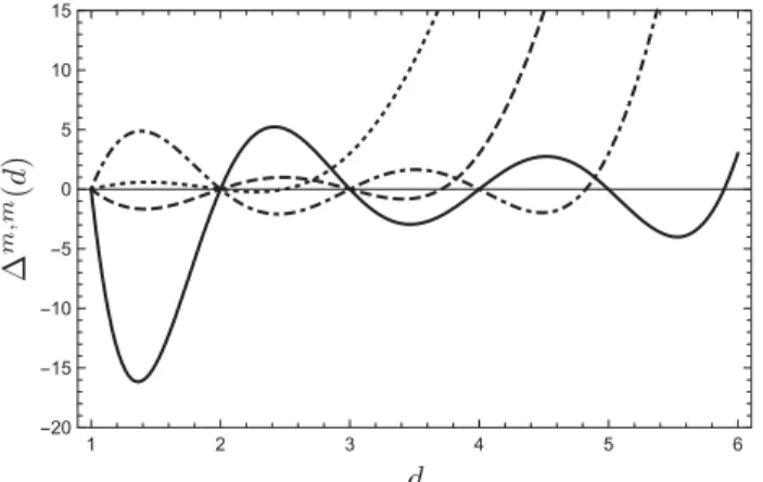
^m;n

is negative valued in some regions (see Fig. 2). A detailed analysis of a

^m;n

shows that jT

^m;m₂

j ≫ jT

^m;m₁

j for m ≫ 1 and therefore gives the main contribution at large m for Δ

^m;m

. The fact that Δ

^m;m

( ∼ C

^m;m

) can become negative valued suggests the possibility of having conformal operators with negative norms. For this reason we compute the one-loop anomalous dimension of the operators O

^ðmÞ

in the next section in order to classify them by their one-loop anoma- lous dimensions.

FIG. 1. Feynman diagrams of leading order.

FIG. 2. Δ

^m;m

ðdÞ, with N

_f

¼ 4 as function of space dimension d for m ¼ 3 , 4, 5, 6 presented by dotted, dashed, dot-dashed, and solid curves, respectively.

2

A nontrivial relation in integer dimensions tr

²

ð I Þ½T

₁

T

⁻¹₂

²

¼ I

serves as an additional check for our results of T

^m;n₁

and T

^m;n₂

.

This relation is obtained from considering the Fierz identities.

(4)

III. ANOMALOUS DIMENSIONS AND UNITARITY IN THE GNY MODEL

So far our calculations are rather general and can be applied to any fermionic theory in noninteger dimensions.

In order to continue our study of norm states in a conformal theory, according to Eq. (10), it is necessary to find eigenstates with definite anomalous dimensions and study correlation functions between them. It is therefore more instructive to consider an explicit example, the GNY model, and compute the one-loop anomalous dimensions of the operators O

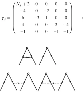
^ðmÞ

defined in Eq. (4) in this model. The Feynman diagrams needed for this calculation are given in Figs. 3 and 4. Note that diagrams in Fig. 4 contribute only to the anomalous dimension of physical operators.

Then it is straightforward to compute these one-loop diagrams and obtain the anomalous dimension matrix γ

^m;n_O

. Interestingly, we find that the anomalous dimension matrix has a simple block diagonal form (the calculation details can be found in Appendix D),

γ

^m;n_O

¼ 2 u

diagðγ

0

; γ

1

; γ

2

; …Þ

^m;n

; ð20Þ where γ

0

is a 5 × 5 anomalous dimension matrix

γ

0

¼ 0 B B B B B B

@

N

_f

þ 2 0 0 0 0

−4 0 −2 0 0

6 −3 1 0 0

4 0 0 2 −4

−1 0 0 −1 −1 1 C C C C C C A

ð21Þ

involving only physical operators, while γ

k≥1

are 2 × 2 matrices

γ

k

¼

2 k þ 2 −2 k − 4 2 k − 1 −2 k − 1

ð22Þ describing the mixing between evanescent operators O

^ð2kþ3Þ

and O

^ð2kþ4Þ

at one-loop order.

It is clear from the explicit expression of the anomalous dimension matrix that the physical and evanescent oper- ators decouple at one-loop order. We can therefore study them separately and find the conformal basis in each case.

Let us write the physical operators in conformal basis as O ˜ . Then

0 B B B B B B B B

@ O ˜

^ð0Þ₀

O ˜

^ð1Þþ

O ˜

^ð1Þ₋

O ˜

^ð2Þþ

O ˜

^ð2Þ₋

1 C C C C C C C C A

¼ 0 B B B B B B B B

@

1 0 0 0 0

1−N10f

−1 1 0 0 0 3 = 2 1 0 0

5

N_f−1

0 0 −1 1

0 0 0 1 = 4 1 1 C C C C C C C C A

0 B B B B B B B B

@ O

^ð0Þ

O

^ð1Þ

O

^ð2Þ

O

^ð3Þ

O

^ð4Þ

1 C C C C C C C C A

ð23Þ

where the operators O ˜

^ð0Þ₀

, O ˜

^ðkÞþ

, and O ˜

^ðkÞ₋

have anomalous dimension γ

₀

¼ 2ðN

f

þ 2Þu , γ

þ

¼ 6 u

, and γ

₋

¼ −4 u

at one-loop order, respectively. Note that we use the bold font letters for anomalous dimension matrices and common ones for the eigenvalues.

The conformal basis for evanescent operators, denoted as O ¯

^ðkÞ

, is

O ¯

^ðkÞþ

O ¯

^ðkÞ₋

!

¼ −1 1

2ðkþ2Þ1−2k

1 ! O

^ð2kþ3Þ

O

^ð2kþ4Þ

!

; ð24Þ with k ≥ 1 and O ¯

^ðkÞ

having anomalous dimension 6 u

and

−4 u

, respectively. These results allow us to classify the operators by their one-loop anomalous dimension. More explicitly, the evanescent operators form two and the physical operators form three classes (two for N

_f

¼ 1 ).

At this point one should mention that the two-loop anomalous dimensions of the operators O

^ðmÞ

probably allow us to make further classifications. The anomalous dimensions of the different operators are collected in Table I.

In order to find the negative norm states of the theory, we have to consider correlation functions between operators of the same anomalous dimension. According to Eq. (10), this corresponds to the study of the coefficient C

_γ

. We point out FIG. 3. Feynman diagrams for calculating anomalous dimen-

sions of evanescent operators.

FIG. 4. Additional Feynman diagrams contributing to the anomalous dimensions of physical operators.

TABLE I. Anomalous dimensions (AD) of the different physi- cal and evanescent operators.

O ˜

^ð0Þ₀

O ˜

^ðkÞþ

O ˜

^ðkÞ−

O ¯

^ðkÞþ

O ¯

^ðkÞ−

AD γ

0

γ

þ

γ

−

γ

þ

γ

−

(5)

that at one-loop accuracy, the orthogonality condition in Eq. (10) is realized by the expressions

hð O ˜

^ðk₀_;¹^Þ

ðxÞÞ

^†

O ˜

^ðk∓²^Þ

ð0Þi ¼ OðϵÞ;

hð O ˜

^ðk_0;¹^Þ

ðxÞÞ

^†

O ¯

^ðk∓²^Þ

ð0Þi ¼ OðϵÞ;

hð O ¯

^ðk¹^Þ

ðxÞÞ

^†

O ¯

^ðk∓²^Þ

ð0Þi ¼ Oðϵ

²

Þ; ð25Þ which is exactly what we find from Eqs. (15), (17), and (18).

With the orthogonality condition checked at the one-loop order, let us now focus on the evanescent operators in the conformal basis. We write the correlator as

hð O ¯

^ðk¹^Þ

ðxÞÞ

^†

O ¯

^ðk²^Þ

ð0Þi ¼ A

⁴

N

_f

jx

²

j

^2d−2

Δ ¯

^k¹^;k²

þ Oðϵ

²

Þ;

Δ ¯

^k¹^;k²

¼ N

_f

T

^k₁¹^;k²

þ T

^k₂¹^;k²

: ð26Þ Here both T

₁

and T

₂

are proportional to ϵ and corre- spond to the first and second diagram in Fig. 1, respec- tively. A is defined in Eq. (14).

The matrices T

₁

are diagonal matrices. It is easy to see that all matrix elements of T

₁₋

ðT

_1þ

Þ are positive (negative) numbers. This implies that ðf; T

₁₋

fÞ > 0 and ðf; T

_1þ

fÞ < 0 for arbitrary nonzero vectors f, i.e., T

₁₋

(T

_1þ

) is a positive (negative) definite matrix. The situation with the matrices T

₂

is a bit more complicated since they are not diagonal. But we checked numerically

³

to confirm that all truncated matrices T

^N₂

¼ ðT

₂

Þ

^n;m

with n; m ≤ N are positive definite (T

_2þ

) and negative definite (T

₂₋

) matrices for N ≤ 80 . The definiteness of T

_1;2

implies

(1) In the large N

_f

limit, the matrices Δ ¯ ∼ T

₁

ð1 þ Oð1 =N

_f

ÞÞ and therefore

Δ ¯

þ

is negative definite, and Δ ¯

₋

is positive definite.

(2) On the contrary, for small values of N

_f

(N

_f

≲ 5), jT

₂

j dominates over jT

₁

j and

Δ ¯

þ

is positive definite, and Δ ¯

₋

is negative definite.

As we have seen, the one-loop corrections are not enough to resolve the operator mixing since infinitely many operators have the same anomalous dimension at one loop.

Nevertheless, it allows one to argue that a general conformal operator with anomalous dimension γ

þ

¼ 6 u

þ Oðϵ

²

Þ has the form

⁴

O

_γ_þ

¼ X

c

^þ_i

O ¯

^ðiÞþ

þ X

c

⁻_j

O ¯

^ðjÞ₋

; ð27Þ where the coefficients c

^þ_i

∼ Oð1Þ, while c

⁻_k

∼ OðϵÞ. One can easily see that the coefficient C

_γ_þ

, corresponding to the correlator of such operators, is given by

C

_γ_þ

¼ A

⁴

N

_f

jx

²

j

^2d−2

ðc

^þ

; Δ ¯

þ

c

^þ

Þ þ Oðϵ

²

Þ: ð28Þ Similarly, for a conformal operator with anomalous dimen- sion γ

₋

¼ −4 u

þ Oðϵ

²

Þ, one gets

C

_γ₋

¼ A

⁴

N

_f

jx

²

j

^2d−2

ðc

⁻

; Δ ¯

₋

c

⁻

Þ þ Oðϵ

²

Þ: ð29Þ As we have shown, the coefficients C

_γ_þ

and C

_γ₋

have opposite signs at order OðϵÞ

⁵

for either small N

_f

or N

_f

→ ∞ . Therefore, one class of the operators inevitably generates the negative norm states of the theory, according to the criteria given in Ref. [1]. In particular, at the lower bound of N

_f

¼ 1, all negative norm states are generated by O ¯

^ðiÞ₋

. In this case, the fermion field has only one degree of freedom and the GNY model may become supersymmetric as suggested in Ref. [33].

We then conclude that the negative norm states are an integral part of the GNY model in d ¼ 4 − 2ϵ dimensions.

At one-loop order, all negative norm states are generated by operators with anomalous dimension γ

₋

for N

_f

≲ Oð1Þ. We believe the negative norm states exist in other theories with fermionic degrees of freedom in noninteger dimensions as well because Eqs. (15), (17), and (18) are valid for any fermionic theory with any number of flavors.

IV. CONCLUSION

We have demonstrated the existence of negative norm states in the Gross-Neveu-Yukaw model in d ¼ 4 − 2ϵ dimensions through the study of the two-point correlation functions of four-fermion operators and their one-loop anomalous dimension matrix. The negative norm states we found are unavoidable, as the two-point correlation functions are an integral part of the theory. They are generated by evanescent operators with anomalous dimension −4 u

at one-loop order when the fermion flavor number is small. We argue that the negative norm states are a general feature of fermionic theories in noninteger dimensions.

It is now clear that unitarity violation occurs in both the scalar and fermionic case. In addition, a recent study also reveals that unitarity is violated in noninteger dimensional nonrelativistic conformal field theory [34], where unitarity is defined by the notion of reflection positivity. Therefore, it seems that unitarity violation is a general property of CFTs in noninteger dimensions.

3

It is possible to show that all the leading principal minors of T

_2þ

are positive, while the k-th order leading minor of T

₂₋

is negative (positive) for odd (even) k.

4

For the sake of clarity one should mention that the mixing with physical operators is here neglected. But it can be shown that the effect of the physical operators is at order O ð ϵ

²

Þ by considering the orthogonality condition of the conformal oper- ators. More specifically, one finds that the coefficients in front of

the physical operators are at O ð ϵ Þ order.

⁵

This is because Δ ¯ are order O ð ϵ Þ.

(6)

We can ’ t see any way to consistently remove these negative norm states from the fermionic field theory in noninteger dimensions. They have no effect, however, on theories in integer dimensions where all the negative norm states vanish.

One should mention, however, that although the loss of unitarity prohibits imposing extra constraints while applying the bootstrap technique, the “ non-unitary boot- strap ” technique, which has no reliance on unitarity, still works [35 – 37].

It would be a natural extension of our current study to compute the two-loop anomalous dimension matrix and investigate how the operators in the conformal basis at the two-loop order further classify the negative and positive norm states. It would be interesting to investigate the appearance of negative norm states in other fermion/scalar conformal field theories as well.

ACKNOWLEDGMENTS

The authors are grateful for insightful discussions with Vladimir Braun and Alexander Manashov. Y. J. acknowl- edges the Deutsche Forschungsgemeinschaft for support under Grant No. BR 2021/7-1.

APPENDIX A: GENERAL FORMULAE We provide some key steps in our calculations. The Feynman diagrams in Fig. 1 are translated into T

^m;n₁

and T

^m;n₂

in Eq. (16) as

T

^m;n₁

¼ δ

m;n

x

⁴

tr

²

ðI

d

Þðm !Þ

²

½trðΓ

^ðmÞμ

= xΓ

^ðmÞν

= xÞ

²

; T

^m;n₂

¼ −1

x

⁴

trðI

d

Þm!n! trð= xΓ

^ðmÞμ

= xΓ

^ðnÞν

= xΓ

^μ_ðmÞ

= xΓ

^ν_ðnÞ

Þ; ðA1Þ where Γ

^ðmÞμ

and alike (e.g., Γ

^ðnÞν

and etc.,) are given in Eq. (5) with arbitary integer m; n and indices μ ; ν . Two identities which proved to be the most useful in our study are

γ

^ν

Γ

^μ¹^…μⁿ

¼ Γ

^νμ¹^…μⁿ

þ X

ⁿ

i¼1

ð−1Þ

^iþ1

g

^νμⁱ

Γ

^μ¹^…ˆ^μⁱ^…μⁿ

; ðA2Þ

ð−1Þ

ⁿ

Γ

^μ¹^…μⁿ

γ

^ν

¼ Γ

^νμ¹^…μⁿ

þ X

ⁿ

i¼1

ð−1Þ

ⁱ

g

^νμⁱ

Γ

^μ¹^…ˆ^μⁱ^…μⁿ

: ðA3Þ

Here μ ˆ

i

denotes that the index μ

i

is omitted. These equations are a consequence of the basic anticommutation relation between gamma matrices and the antisymmetric structure of Γ

^μ_ðnÞ

. By combining the latter two equations one finds

2Γ

^νμ¹^…μⁿ

¼ γ

^ν

Γ

^μ¹^…μⁿ

þ ð−1Þ

ⁿ

Γ

^μ¹^…μⁿ

γ

^ν

: ðA4Þ The general formula for contracting the antisymmetrized products of gamma matrices reads

Γ

^ν¹^…ν^m^μⁿ^…μ¹

Γ

μ1…μn

¼ Y

ⁿ⁻¹

i¼0

ðd − m − iÞΓ

^ν¹^…ν^m

: ðA5Þ

Finally, we have

x

_a

x

_b

Γ

^μ¹^{…a…b…ν}^m

¼ 0; ðA6Þ as a direct consequence of the definition of Γ

^μ¹^{…a…b…ν}^m

.

We then calculate T

^m;n₁

and T

^m;n₂

separately in the following two sections.

APPENDIX B: T

^m;n₁

The cyclic property of the trace together with the anticommutation relation between gamma matrices allows us to first conclude that T

^m;n₁

¼ 0 for m ≠ n. One thus writes,

T

^m;n₁

¼ δ

m;n

x

⁴

tr

²

ðI

d

Þðm !Þ

²

½trðΓ

^ðmÞμ

= x Γ

^ðmÞν

= xÞ

²

;

¼ B

_m

δ

m;n

ðm !Þ

²

: ðB1Þ

Then we note B

_m

¼ 1

tr

²

ðI

d

Þ trðΓ

^ðmÞμ

Γ

^ðmÞν

ÞtrðΓ

^μ_ðmÞ

Γ

^ν_ðmÞ

Þ; ðB2Þ which can be proven by the cyclic property of the trace together with Eqs. (A2) and (A6).

By setting the default ordering of Γ

^m_μ

and Γ

^ðmÞν

to be μ

1

; … ; μ

m

and ν

1

; …ν

m

, while noting μ

i

≠ μ

j

and ν

i

≠ ν

j

for i ≠ j, B

_m

can then be rewritten as B

_m

¼ 1

tr

²

ðI

d

Þ trðγ

_μ₁_…μ_m

γ

_ν₁_…ν_m

Þtrðγ

^μ¹^…μ^m

γ

^ν¹^…ν^m

Þ

¼ R

_μ₁_…ν_m

R

^μ¹^…ν^m

: ðB3Þ By moving γ

μ₁

to the right of the product in Eq. (B3) and using the cyclic property of the trace, one finds

R

_μ₁_…ν_m

¼ ð−1Þ

^m−1

trðI

d

Þ

X

^m

i¼1

ð−1Þ

^iþ1

g

_μ₁_ν_i

× trðγ

μ2…μm

γ

ν1…ˆνi…νm

Þ;

ðB4Þ where again ν ˆ

i

denotes the omitted index.

Here we have reduced a trace with 2 m indices to a sum of

traces with 2ðm − 1Þ indices. By repeatedly applying

Eq. (B4) one can reduce the trace with 2m indices to

trðI

d

Þ with an appropriate combination of coefficients. It is

clear that each further reduction step produces one extra

summation and one extra set of g

^μ^ik^ν^jl

with the appropriate

sign in front. To this end, we write,

(7)

R

_μ₁_…ν_m

¼ ð−1Þ

^m²^ðm−1Þ

trðI

d

Þ X

^m

i₁¼1

… X

^m

i_m¼1

g

_μ₁_ν_i

1

…

× g

_μ_m_ν

im

Ωði

₁

; … ; i

_m

Þ

; ðB5Þ

where the overall factor ð−1Þ

^m²^ðm−1Þ

is accumulated from the repeated use of Eq. (B4) and Ωði

₁

; … ; i

_m

Þ ∈ f0 ; 1g. Since each index ν

k

appears only once in the trace, one straightfor- wardly concludes that Ωði

₁

; …; i

k

; …; i

k

; …; i

m

Þ ¼ 0. A more detailed analysis also reveals that Ωði

1

; … ;i

_k

;i

_kþ1

; … ;i

_m

Þ ¼

−Ωði

₁

; … ;i

_kþ1

;i

_k

; … ;i

_m

Þ, which is a property inherited from the antisymmetric nature of Γ

^ðmÞ

. Finally by noting that Ωð1; …; mÞ ¼ 1, which corresponds to eliminate γ

ν1

; γ

ν2

; … ; γ

νm

in order, one identifies

Ωði

₁

; … ; i

_m

Þ ¼ ϵ

i₁…im

: Therefore, one finds

B

_m

¼ X

^m

i1;…;im¼1 j1;…;jm¼1

mg

^μ_μⁱ_j¹₁

…g

^μμ^im_jm

ϵ

i₁…im

ϵ

^j¹^…j^m

; ðB6Þ

with

X

^m

i1;…;im¼1 j1;…;jm¼1

≡ X

^m

i₁¼1

… X

^m

im¼1

X

^m

j₁¼1

… X

^m

jm¼1

: ðB7Þ

This summation can be worked out by dividing the general case into two scenarios:

i

_k

¼ j

_k

¼ m; k ¼ 1 ; … m;

or i

_k

¼ j

_l

¼ m; k ≠ l; m; l ¼ 1 ; … m: ðB8Þ The summation is then easily carried out and leads to a recurrence relation for B

_m

,

B

_m

¼ mðd − m þ 1ÞB

_m−1

; ðB9Þ for m > 1 . Combined with the initial condition of the sequence B

₀

¼ 1 , we obtain the final expression for T

^m;n₁

,

T

^m;n₁

¼ Γðd þ 1Þ

m !Γðd − m þ 1Þ δ

m;n

: ðB10Þ It is clear that T

^m;n₁

vanishes for theories in even d dimensions if m > d. This observation is in accordance with the fact that there are d numbers of gamma matrices in even d dimensions, and consequently, the antisymmetrized product of m gamma matrices Γ

^ðmÞμ

vanishes if m > d. In odd dimension d, Γ

^ðdÞ

is no longer an independent matrix since Γ

^ðdÞ

∝ Γ

^ð0Þ

, and therefore this redundancy must be removed “ by hand. ” If the dimension d is no longer an integer, however, then T

^m;n₁

never vanishes and can take negative values.

APPENDIX C: T

^m;n₂

We proceed to calculate T

^m;n₂

T

^m;n₂

¼ −1

x

⁴

trðI

d

Þm ! n ! trð= x Γ

^ðmÞμ

= x Γ

^ðnÞν

= x Γ

^μ_ðmÞ

= x Γ

^ν_ðnÞ

Þ; ðC1Þ which can be simplified using Eqs. (A2) – (A6) as

T

^m;n₂

¼ −1

trðI

d

Þm ! n ! trðΓ

^ðmÞμ

Γ

^ðnÞν

Γ

^μ_ðmÞ

Γ

^ν_ðnÞ

Þ: ðC2Þ Then again with Eqs. (A4) and (A5), one finds

T

^m;n₂

¼ −1

2 trðI

d

Þm ! n ! tr½Γ

^ν²^…νⁿ

Γ

^ðmÞ

γ

ðnÞ

Γ

ðmÞ

γ

^ν¹

þ ð−1Þ

^mþn⁻¹

ðd − 2 mÞΓ

^ðn^−1Þ

Γ

^ðmÞ

γ

ðn−1Þ

Γ

ðmÞ

¼ −1

2 trðI

d

Þm ! n ! ðs

₁

þ s

₂

Þ; ðC3Þ where γ

_ðn−kÞ

¼ γ

_ν₁_…ν_n−k

¼ γ

_ν₁

…γ

_ν_n−k

is a product of gamma matrices of standard ordering. Then,

s

₁

¼ tr

2 X

ⁿ⁻¹

i¼1

ðd − n þ 2ÞΓ

^ðn−2Þ

Γ

^ðmÞ

γ

_ðn−2Þ

Γ

ðmÞ

þ ð−1Þ

^mþn−1

ðd − 2mÞΓ

^ðn−1Þ

Γ

^ðmÞ

γ

_ðn−1Þ

Γ

ðmÞ

: ðC4Þ One then obtains a recursion relation for T

^m;n₂

,

T

^m;n₂

¼ ð−1Þ

^mþn−1

ðd − 2 mÞT

^m;n−1₂

þ ðn − 1Þðd − n þ 2ÞT

^m;n−2₂

; ðC5Þ with boundary conditions

T

^m;0₂

¼ − ð−1Þ

^m²^ðm−1Þ

m!

Γðd þ 1Þ Γðd − m þ 1Þ ; T

^m;1₂

¼ − ð−1Þ

^m²^ðmþ1Þ

m!

ðd − 2 mÞΓðd þ 1Þ

Γðd − m þ 1Þ : ðC6Þ The recurrence relation can be expressed as

T

^m;n₂

¼ − 1

2 i

mðmþ1Þþnðnþ1Þ

a

_m;n

; ðC7Þ where a

_m;n

are the coefficients of the generating function

Fðx; yÞ ¼ X

^∞

m;n¼0

a

_m;n

x

^m

y

ⁿ

: ðC8Þ Then the recursive behavior in Eq. (C5) is inherited by a

_m;n

and combined with the boundary conditions Eq. (C6).

The generating function is found to be

Fðx; yÞ ¼ ð1 − xþ yþ xyÞ

^d

þ ð1 þ x − y þ xyÞ

^d

− ð1 þ x þ y − xyÞ

^d

þ ð1 − x − y − xyÞ

^d

: ðC9Þ

(8)

APPENDIX D: ANOMALOUS DIMENSIONS The Feynman diagrams in the first row of Fig. 3 have a divergent part which reads

I

^ðmÞ₁

¼ ðg

₁

Þ

²

m − 2

16π

²

ϵ ð−1Þ

^m

O

^ðmÞ

: ðD1Þ The Feynman diagrams in the last row of Fig. 3 together yield

I

^ðmÞ₂ ^div

¼ ðg

₁

Þ

²

64π

²

m !ϵ ΨðxÞ½Γ ¯

^ðmÞ

; γ

μ

ΨðxÞ

× ΨðxÞ½Γ ¯

ðmÞ

; γ

^μ

ΨðxÞ; ðD2Þ which requires some algebra. For odd m, we get

I

^ðm¼oddÞ₂

¼ ðg

₁

Þ

²

ðm þ 1Þ

16π

²

ϵ O

^ðmþ1Þ

; ðD3Þ while for the even case, we have

I

^ðm¼evenÞ₂

¼ ðg

₁

Þ

²

ð5 − mÞ

16π

²

ϵ O

^ðm−1Þ

: ðD4Þ The Feynman diagrams in Fig. 4 yield a divergent piece which reads

I

^ðmÞ₃

¼ ðg

₁

Þ

²

O

^ð0Þ

16π

²

ϵ

ð−1Þ

^mðm−1Þ=2

m !

Y

m−1 i¼0

ð4 − iÞ − N

_f

δ

_m;0

: ðD5Þ

Consequently, the operator renormalization matrix is found to be

Z

^m;n_O

¼ I

₁

þ I

₂

þ I

₃

¼ ðg

₁

Þ

²

16π

²

ϵ

ðn − 2Þð−1Þ

ⁿ

δ

m;n

þ n δ

_m;n−1

modðm; 2Þ þ ð4 − nÞδ

^m;nþ1

modðn; 2Þ − N

_f

δ

_m;0

δ

_n;0

þ 4!ð−1Þ

^mðm−1Þ=2

m!ð4 − mÞ! δ

n;0

: ðD6Þ

The one-loop renormalization of the fermion self energy in the GNY model reads

Z

^m;n_Ψ

¼ 1 þ ðg

₁

Þ

²

32π

²

ϵ δ

m;n

; ðD7Þ and therefore one obtains the one-loop anomalous dimen- sions matrix

γ

^m;n_O

¼ d α

₁

d ln μ

∂

∂α

1

lnðZ

_O

Z

⁻²_Ψ

Þ

¼ 2 u

ð1 − ð−1Þ

ⁿ

ðn − 2ÞÞδ

m;n

− n δ

_m;n−1

modðm; 2Þ þ ðn − 4Þδ

_m;nþ1

modðn; 2Þ þ N

_f

δ

_m;0

δ

_n;0

− 4!ð−1Þ

^mðm−1Þ=2

m !ð4 − mÞ! δ

_n;0

: ðD8Þ

[1] M. Hogervorst, S. Rychkov, and B. C. van Rees, Phys. Rev.

D 93, 125025 (2016).

[2] A. M. Polyakov, Zh. Eksp. Teor. Fiz. 66, 23 (1974) [Sov. Phys. JETP 39, 9 (1974)].

[3] S. Ferrara, A. F. Grillo, and R. Gatto, Ann. Phys. (N.Y.) 76, 161 (1973).

[4] R. Rattazzi, V. S. Rychkov, E. Tonni, and A. Vichi, J. High Energy Phys. 12 (2008) 031.

[5] S. Rychkov, arXiv:1111.2115.

[6] S. El-Showk, M. F. Paulos, D. Poland, S. Rychkov, D.

Simmons-Duffin, and A. Vichi, Phys. Rev. D 86, 025022 (2012).

[7] F. Kos, D. Poland, and D. Simmons-Duffin, J. High Energy Phys. 06 (2014) 091.

[8] V. S. Rychkov and A. Vichi, Phys. Rev. D 80, 045006 (2009).

[9] F. Caracciolo and V. S. Rychkov, Phys. Rev. D 81, 085037 (2010).

[10] D. Poland and D. Simmons-Duffin, J. High Energy Phys. 05 (2011) 017.

[11] R. Rattazzi, S. Rychkov, and A. Vichi, Phys. Rev. D 83, 046011 (2011).

[12] R. Rattazzi, S. Rychkov, and A. Vichi, J. Phys. A 44, 035402 (2011).

[13] A. Vichi, J. High Energy Phys. 01 (2012) 162.

[14] Y. Nakayama and T. Ohtsuki, Phys. Lett. B 734, 193 (2014).

[15] Z. Li and N. Su, J. High Energy Phys. 04 (2017) 098.

[16] J. B. Bae and S. J. Rey, arXiv:1412.6549.

[17] D. Poland, D. Simmons-Duffin, and A. Vichi, J. High Energy Phys. 05 (2012) 110.

[18] S. El-Showk and M. F. Paulos, Phys. Rev. Lett. 111, 241601 (2013).

[19] K. G. Wilson and M. E. Fisher, Phys. Rev. Lett. 28, 240 (1972).

[20] K. G. Wilson, Phys. Rev. D 7, 2911 (1973).

[21] M. V. Kompaniets and E. Panzer, Phys. Rev. D 96, 036016 (2017).

[22] S. El-Showk, M. Paulos, D. Poland, S. Rychkov, D.

Simmons-Duffin, and A. Vichi, Phys. Rev. Lett. 112,

141601 (2014).

(9)