Higher-spin currents in the Gross-Neveu model at 1/n 2

JHEP01(2017)132

Published for SISSA by Springer

Received: October 28, 2016 Accepted: January 8, 2017 Published: January 30, 2017

Higher-spin currents in the Gross-Neveu model at 1/n ²

A.N. Manashov^a,b and E.D. Skvortsov^c,d

aInstitut f¨ur Theoretische Physik, Universit¨at Hamburg, Hamburg, D-22761 Germany

bInstitut f¨ur Theoretische Physik, Universit¨at Regensburg, Regensburg, D-93040 Germany

cArnold Sommerfeld Center for Theoretical Physics, Ludwig-Maximilians University Munich, Theresienstr. 37, Munich, D-80333 Germany

dLebedev Institute of Physics,

Leninsky ave. 53, Moscow, 119991 Russia E-mail: alexander.manashov@desy.de, evgeny.skvortsov@physik.uni-muenchen.de

Abstract:

We calculate the anomalous dimensions of higher-spin currents, both singlet and non-singlet, in the Gross-Neveu model at the 1/n

²

order. It was conjectured that in the critical regime this model is dual to a higher-spin gauge theory on AdS

4

. The AdS/CF T correspondence predicts that the masses of higher-spin fields correspond to the scaling dimensions of the singlet currents in the Gross-Neveu model.

Keywords:

1/N Expansion, Conformal Field Theory, AdS-CFT Correspondence

ArXiv ePrint: 1610.06938

In honour of Alexander A. Andrianov’s 70th birthday

JHEP01(2017)132

Contents

1 Introduction

1

2 GN model in

d

dimensions

2

3 Higher-spin currents

6

3.1 Non-singlet currents at 1/n

² 8

3.1.1 Anomalous dimensions

8

3.2 Singlet currents at 1/n

² 9

3.2.1 Anomalous dimensions

9

3.3 Conformal spin expansion

10

3.3.1 Conformal spin expansion of non-singlet currents

11

3.3.2 Conformal spin expansion of singlet currents

11

3.4 Three dimensions and higher-spin masses

12

4 Summary

14

A Renormalized propagators

15

B Numerical values

15

1 Introduction

Since its introduction in 1974 [1] the Gross-Neveu (GN) model serves as a toy model for studies of many interesting physical phenomena. In particular, the GN model in 2 < d < 4 dimensions possesses the Wilson-Fisher fixed point. In the critical regime this model enjoys scale and conformal invariance and provides an example of nontrivial conformal field theory (CFT). Various critical indices in the GN model were calculated both in the 2 + and 1/N expansions (here N is the number of the fermion field components), see e.g. refs. [2–11].

Due to its simplicity, the GN model together with the O(N ) symmetric ϕ

⁴

model presents an ideal playground for testing new techniques in CFTs [12–26].

In this work we compute the anomalous dimensions γ

s

of the specific composite oper- ators, known as higher-spin currents:

J

s

≡ J

µ1...µs

= ¯ q

^a

γ

µ1

∂

µ2

. . . ∂

µs

q

^a

+ . . . . (1.1)

Here s is the spin and q is the N −component Dirac fermion while the ellipses stand for

the total derivative terms and symmetrization over all indices and subtraction of traces

are implied. In the free field approximation all the higher-spin currents are conserved and

give rise to an infinite-dimensional symmetry, known as the higher-spin symmetry, which

is then broken by interactions, see e.g. refs. [13,

17,18,27].

JHEP01(2017)132

At the 1/N order the anomalous dimension of the current J

_s

have been calculated in 1977 by Muta and Popov´ıc [28]. In this work we extend this calculation to the next order using the technique developed in [29–31]. As a nontrivial check of our result we verify that the structure of an asymptotic expansion of the anomalous dimension as a function of the conformal spin, j = s − 1 + (d + γ

s

)/2, agrees with the predictions of refs. [32–34].

Another surge of recent interest to the GN model comes from studies of the AdS/CFT correspondence [35–37]. It was conjectured in [38] that the critical O(N )-vector model is dual to the higher-spin gauge theory in AdS

4

. Shortly after, the conjecture was extended to the GN model and its super-symmetric extensions [39,

40]. Some non-trivial tests of

this conjecture were performed at the level of three-point functions [41] and at the level of one-loop determinants, see [42,

43] for a discussion and references. Remarkably, the same

AdS

₄

higher-spin theory should be dual both to free and interacting models, depending on the boundary conditions. Moreover, there is a continuous transition between fermionic and bosonic versions of these CFT’s, i.e. the three-dimensional bosonization [27,

44,45],

which on the AdS side is accounted for by a free parameter of the higher-spin theory and on the CFT side is realized via coupling to the Chern-Simons sector [44]. While the duality at the tree level is better supported, the most subtle effects should come from the loops.

According to [46], see also [17,

47,48], radiative corrections on the AdS side should generate

masses δm

²

of the higher-spin fields that from the CFT point of view correspond to the anomalous dimensions γ

_s

of the higher-spin currents

m

²_s

= m

²₀

(s) + δm

²_s

, m

²₀

(s) = (d + s − 2)(s − 2) − s, δm

²_s

= γ

_s

d − 4 + 2s + γ

_s

, (1.2) The masses are measured in the units of the cosmological constant. Therefore, our results should be equivalent to two-loop computations in the higher-spin theory. More specifically, one should be able to extract γ

s

from the logarithmic corrections to the near boundary behaviour of higher-spin fields.

The paper is organized as follows: in section

2

we recall the definition of the GN model and briefly review the method to compute the critical exponents. The section

3

contains our results and some details of calculations for the anomalous dimensions of the higher- spin currents at the next-to-leading order in 1/N . The renormalized propagators can be found in appendix

A, while some of the numerical values of the anomalous dimensions are

collected in appendix

B.

2 GN model in d dimensions

The GN model with U(N ) symmetry describes a system of d (d ≡ 2µ)-dimensional N- component Dirac fermions, q (¯ q) ≡

q

^a

(¯ q

^a

), a = 1, . . . , N . Its action (in Euclidean space) takes the form

¹

[1]

S = −

Z

d

^d

x

h

¯

q

∂q + g

2N (¯ qq)

²i

. (2.1)

1The discussion of the issues related to renormalization of this model in 2 +dimensions can be found in refs. [11,49–52].

JHEP01(2017)132

To generate a systematic 1/N expansion it is convenient to introduce an auxiliary scalar field σ and rewrite GN action (2.1) in the following form:

S = −

Z

d

^d

x

¯

q

∂q + σ qq ¯ − N 2g σ

²

. (2.2)

At a certain value of the coupling g = g

∗

the system undergoes the second order phase transition [53]. For g < g

∗

the expectation value of σ field vanishes, σ

₀

= hσi = 0, and the fermions are massless, while for g > g

∗

hσi 6= 0 and fermions acquire mass, m = hσi at the leading order. At the critical point, g = g

∗

, the correlators of the fields q, q, σ ¯ exhibit power law behaviour and, as it can be shown, the model enjoys scale and conformal invariance [6].

Critical exponents are usually calculated with the help of the self-consistency equations [54]

or the conformal bootstrap [55] methods (see ref. [56] for a review). However, it turns out that for the analysis of the operators with nontrivial tensor structure it is more convenient to use another approach described below.

In the infrared region (IR) (momenta much less than the cutoff Λ) the dominant contribution to the propagator of the σ field in the leading order comes from the fermion loop [53]

D

σ

(p) = − 1

n b(µ)/(p

²

)

^µ−1

, D

σ

(x) = − 1

n B(µ)/x

²

. (2.3) Here n = N × tr

1

, where tr

1

is a trace of the unit matrix in the space of d-dimensional spinors

²

and the normalization factors are

b(µ) = (4π)

^µ

Γ(2µ − 1)

Γ

²

(µ)Γ(1 − µ) , B(µ) = 4Γ(2µ − 1)

Γ

²

(µ)Γ(µ − 1)Γ(1 − µ) . (2.4) For practical calculations it is convenient to use a simplified (massless) version of the GN model which is critically equivalent to (2.2). The action of the model is given by the following expression [29,

56]

S

⁰

= −

Z

d

^d

x

¯ q

∂q − 1

2 σLσ + σ qq ¯ + 1 2 σLσ

. (2.5)

The kernel L is the inverse σ-propagator (2.3), L

⁻¹

= D

_σ

. It has the form L(x) = tr D

_q

(x)D

_q

(−x) = −n

Γ(µ) 2π

^µ

2

1

(x

²

)

^2µ−1

, D

_q

(x) = − Γ(µ) 2π

^µ

x

[x

²

]

^µ

, (2.6) where D

_q

(x) is the fermion propagator.

The first two terms in (2.5) are considered as the free part of the action, S

₀

, and the remaining ones — as an interaction, S

int

. The last term in (2.5) cancels diagrams with insertions of simple fermion loops in the σ-lines. Of course, for giving a sense to the model (2.5) it is necessary to introduce a regularization. Indeed, it can be easily checked that the vertex σ qq ¯ diverges logarithmically in any dimensions. A regularization preserving

2This trace does not have (and does not require) an exact expression in terms of d (for the integer dimensionsd= 2,3,4 it is usually assumed that tr1= 2,2,4).

JHEP01(2017)132

the masslessness of propagators, that is important for practical calculations, was proposed in [29]. Namely, in order to make diagrams finite it is sufficient to change the kernel L in the free part of the action, S

₀

, as follows

L(x) → L

∆

(x) = L(x)(M

²

x

²

)

^−∆

C

⁻¹

(∆) ∼ x

^{−2(2µ−1+∆)}

. (2.7) Here M is the scale parameter and C(∆) is an arbitrary function regular at ∆ = 0 such that C(0) = 1. The choice of the function C(∆) affects only the normalization of correlators but not their scaling dimensions.

The UV divergences appear in diagrams as poles in ∆ and are removed by the corre- sponding counterterms. The renormalized action (2.5) takes the form

S

_R⁰

= −

Z

d

^d

x

Z

1

q ¯

∂q − 1

2 σL

_∆

σ + Z

2

σ qq ¯ + 1 2 σLσ

. (2.8)

The model is not, however, multiplicatively renormalized, i.e. S

_R⁰

(q, σ) 6= S

⁰

(q

0

, σ

0

). This means that the anomalous dimensions of the fields or composite operators are not related directly to the corresponding renormalization factors. The multiplicative renormalizability can be restored in the extended model by introducing two new charges [29],

S

_R⁰

(u, v) = −

Z

d

^d

x

h

Z

1

(u, v)¯ q

∂q − u

2 σL

∆

σ + Z

2

(u, v)σ qq ¯ + v 2 σLσ

i

, (2.9)

so that S

_R⁰

(q, σ, u, v) = S

⁰

(q

0

, σ

0

, u

0

, v

0

). Obviously, for u = v = 1 the extended model coincides with the model (2.8). Since the model (2.9) is multiplicatively renormalizable the scale dependence of the Green functions is described by the renormalization group equations (RGEs). For instance, let {O

_i

} be a set of operators which mix under renormalization. The RGE for the r-point 1PI functions with the insertion of the operators O

_i

takes the form

M ∂

M

+ β

u

∂

u

+ β

v

∂

v

− n

Φ

γ

Φ

δ

^ik

+ γ

^ik_O

Γ

k

(u, v; p, p

1

, . . . , p

r

) = 0 , (2.10) where n

_Φ

= (n

_q

+ n

_q¯

)γ

_q

+ n

_σ

γ

_σ

and the RG functions are defined in the standard way

β

u

= M ∂

M

u , β

v

= M ∂

M

v , γ

Φ

= M ∂

M

ln Z

Φ

, γ

O

= −M ∂

_M

ZZ

⁻¹

. (2.11) Here Z

q

= Z

₁^1/2

, Z

σ

= Z

2

Z

₁⁻¹

and the matrix Z enters the definition of the renormalized operator, O

^R_i

(Φ) = Z

_ik

O

_k

(Φ

0

). In an arbitrary subtraction scheme the term

β

u

∂

u

+ β

v

∂

v

Γ

i

(u, v; {p})

u=v=1

= −2γ

_σ

(∂

u

+ ∂

v

)Γ

i

(u, v; {p})

u=v=1

6= 0 , (2.12) which implies that the RG functions γ

_Φ

, γ

O

are not true anomalous dimensions that de- termine the scale dependence of the correlators. Let us stress that the correlators in the model (2.8) and in the extended model (2.9) at u = v = 1 have certain scaling dimensions, namely

M ∂

M

− n

Φ

γ

_Φ

δ

^ik

+ γ

^ik_O

Γ

k

(u = v = 1; {p}) = 0 , (2.13)

JHEP01(2017)132

but, in general, γ

_Φ

6= γ

_Φ

, γ

_O

6= γ

O

. It was shown in [29] that in the MOM scheme the renormalized Green functions depend only on the difference of the charges u and v, Γ

_k

(u, v; {p})) = Γ

_k

(u − v; {p}). This implies that the term with β-functions in the RGE (2.10) vanishes and, hence, γ

_Φ

= γ

_Φ^MOM

, γ

_O

= γ

_O^MOM

. Unfortunately the calculations in the MOM scheme is hardly feasibly beyond the leading order. In the most suitable for practical calculations MS-scheme, (Z-factors are given by series in 1/∆) in general, γ

_O

6= γ

O

. However as it was shown in [31] the difference is of order 1/n

³

γ

_Φ^∗

= γ

_Φ

− γ

_Φ^MS

= O(1/n

³

) , γ

_O^∗

= γ

_O

− γ

_O^MS

= O(1/n

³

) . (2.14) Thus, the anomalous dimensions in the MS scheme up to 1/n

²

order inclusively can be calculated with the help of eqs. (2.11). Taking into account that

β

u

= 2u ∆ − γ

σ

, β

v

= −2vγ

_σ

(2.15)

one derives (from now on we consider only the MS scheme and omit the label MS) γ

O

= −2

∆u∂

u

− γ

σ

(u∂

u

+ v∂

v

)

Z Z

⁻¹

= −2u∂

_u

Z

⁽¹⁾

(u, v)|

_u=v=1

(2.16) where

Z = 1 +

X

k>0

∆

^−k

Z

^(k)

. (2.17)

Taking into account that there is no derivative with respect v in (2.16) one can put v = 1 from the very beginning

³

arriving to the final expression for anomalous dimensions [31]

γ

O

= −2u∂

_u

Z

⁽¹⁾

(u, 1)

u=1

. (2.18)

Taking into account that the charge u appears only in the σ field propagator D

σ

(x) = − 1

u × 1

n B(µ)C(∆) M

^2∆

(x

²

)

^1−∆

, (2.19)

and −u∂

_u

counts a number of σ lines in diagrams one concludes that the contributions of each diagram to the Z factor and to the anomalous dimension, γ

O

, differ by a factor 2n

_σ

, where n

σ

is the number of internal σ lines in the diagram.

Equations (2.16), (2.18) have a striking resemblance to the analogous expressions in the MS scheme in the dimensional regularization. Being a variation of the standard RG technique, this approach is rather effective for the analysis of composite operators with a nontrivial tensor structure. A more detailed discussion can be found in refs. [31,

57] and a

generalization to gauge theories in refs. [58,

59].

On finishing the review we recall known results for the anomalous dimensions of the fermion and auxiliary fields [7–10]. We adopt the standard notations [56]

η = 2γ

q

, γ

σ

= −η − κ . (2.20)

3In this case,v= 1, there are no diagrams with an insertion of the simple fermion loop into theσlines (it is exactly cancelled by the term 1/2σLσin the action (2.9)).

JHEP01(2017)132

The index η is known with 1/n

³

[9,

10] and

κ with 1/n

²

[7,

9] accuracy. We need the first

two coefficients in the expansion for η, η =

P

k≥1

η

k

/n

^k

, η

1

= −B(µ)/2µ = − 2 Γ(2µ − 1)

Γ(µ + 1)Γ(µ)Γ(µ − 1)Γ(1 − µ) , (2.21)

η

₂

= η

₁²

1 2

1 (µ − 1)

²

(µ − 1)

²

µ + 3µ + 4(µ − 1) + 2(µ − 1)(2µ − 1)Ψ(µ)

, (2.22) where Ψ(µ) = ψ(2µ − 1) − ψ(1) + ψ(2 − µ) − ψ(µ), and only the first one for κ:

κ

₁

= η

₁

µ

µ − 1 , γ

_σ⁽¹⁾

= − 2µ − 1

µ − 1 η

₁

. (2.23)

3 Higher-spin currents

We consider the higher-spin (traceless and symmetric) operators bilinear in fermionic fields:

• the scalar (singlet) operators

O

_s

= ¯ qγ

µ1

∂

µ2

. . . ∂

µs

q + . . . . (3.1)

• the adjoint (non-singlet) operators

O

^A_s

= ¯ q t

^A

γ

_µ1

∂

_µ2

. . . ∂

_µs

q + . . . . (3.2) Here t

^A

are the generators of the SU(N) group and summation over isotopic indices is always implied, (¯ q q = ¯ q

^a

q

^a

). It is assumed that Lorentz indices are symmetrized and traces subtracted so that s is the spin of the operator. The ellipses stand for the total derivatives which can be neglected if one is interested in the anomalous dimensions only.

The renormalized operators take the form

[O

_s

] = Z

_s

O

_s

, [O

_s^A

] = Z

_s^A

O

^A_s

. (3.3) Up to 1/n

²

terms inclusively the anomalous dimensions are given by

γ(s) = η − 2u∂

u

Z

_s⁽¹⁾

u=1

, γ

A

(s) = η − 2u∂

u

Z

_s^A,(1)

u=1

, (3.4)

where Z

⁽¹⁾

is a simple pole in the corresponding renormalization factor Z = 1 + Z

⁽¹⁾

/

∆ + O(1/∆

²

).

For odd s the anomalous dimensions of singlet and non-singlet operators coincide, γ

s

= γ

_s^A

. Therefore, from now on, it will be tacitly implied that spin s is even for the singlet currents.

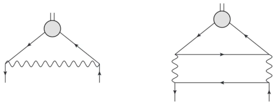
As usual, the renormalization factor Z is extracted from the correlator of the operator with fermion fields at zero momentum transfer, hO(0)q(p)¯ q(p)i. Calculating the leading order (1/n) diagrams shown in figure

1

we reproduce the result of Muta and Popovic [28]

γ

_A

(s) = 1 n η

₁

1 − µ(µ − 1) (s + µ − 1)(s + µ − 2)

+ O(1/n

²

) , (3.5a)

γ(s) = 1 n η

1

1 − µ(µ − 1) (s + µ − 1)(s + µ − 2)

1 + Γ(2µ − 1)s!

Γ(2µ − 3 + s)(µ − 1)

+ O(1/n

²

) .

(3.5b)

JHEP01(2017)132

Figure 1. The leading order diagrams for the correlatorhO(0)q(p)¯q(p)i. The right diagram con- tributes only to the correlator of singlet operators of even spin.

It can be easily checked that the conserved currents, the spin-one and spin-two singlet (the energy-momentum tensor) currents, have vanishing anomalous dimensions, γ

_A

(1) = 0 and γ(2) = 0.

The anomalous dimensions (determined only for integer s) define analytic functions of complex variable (spin) s, which at integer points coincide with the corresponding anoma- lous dimensions. It is well known that such a continuation should be done separately for even and odd s. Thus the eqs. (3.5) define three analytic functions, γ

_A^±

(s) and γ(s), where γ

_A⁺

, γ reproduce the corresponding anomalous dimensions for even s, and γ

_A⁻

(s) for odd s.

Obviously, in the 1/n order, γ

_A⁺

(s) = γ

_A⁻

(s).

In CFTs it is more natural to consider anomalous dimensions as functions of the conformal spin j defined as

j = 1

2 ∆

_s

+ s

= µ − 1 + s + 1

2 γ(s) , (3.6)

where s is the spin and ∆

s

is the scaling dimension of an operator. For a given anomalous dimension γ (s) let us define a function f (j) as follows

f (j) = f

µ − 1 + s + 1 2 γ (s)

= γ(s) . (3.7)

It was noticed in [32] that in all known examples the large j expansion of the function f (j) has a rather specific structure. Let us consider the f -functions for the anomalous dimensions (3.5). They take the form

γ

_A^±

(s) = f

_A^±

(j) = 1 n η

₁

1 − µ(µ − 1) j(j − 1)

+ O(1/n

²

) , γ(s) = f(j) = 1

n η

1

1 − µ(µ − 1) j(j − 1)

1 + Γ(2µ − 1) µ − 1

Γ(j − µ + 2) Γ(j + µ − 2)

+ O(1/n

²

) . (3.8) At the leading order the functions f

_A^±

are invariant under j → 1 − j. The singlet function f (j) is given by the sum of two terms one of which is invariant under j → 1 − j, but another one, ∼ Γ(j − µ + 2)/Γ(j + µ − 2), is not. The asymptotic expansion for this term has the form

j − 1

2

−2(µ−1)

X

k≥0

a

k

(j(j − 1))

^k

. (3.9)

JHEP01(2017)132

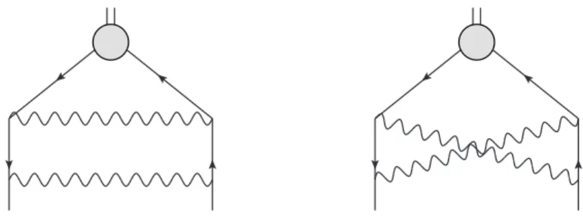
Figure 2. The 1/n² order diagrams for the non-singlet currents.

Therefore, up to the prefactor the series is invariant under j → 1 − j. It was argued in [32–

34] that a generic contribution to the asymptotic expansion of

f(j) has the structure (3.9) where the coefficients a

_k

are allowed to be a function of ln(j − 1/2).

Taking these findings into account we also present our results for the anomalous di- mensions as functions of conformal spin. Besides that the corresponding expressions have a simpler form the very possibility to bring results to the form (3.9) provides a nontrivial check of calculations.

3.1 Non-singlet currents at 1/n

²

Diagrams contributing to the renormalization of the non-singlet current at 1/n

²

order comprise the diagrams with the self-energy (SE) and vertex corrections to the leading order diagram (shown in the l.h.s. of figure

1) plus two additional diagrams shown in figure2. The

calculations are straightforward so that we present the answer only. It is worth emphasizing that any diagram containing a fermion loop with odd number of attached σ lines vanishes, which is exactly the feature that makes computations in the GN model more feasible that in the O(N ) σ-model.

3.1.1 Anomalous dimensions

The full conformal dimension of the non-singlet currents can be written as

∆

_s

= ∆

⁽⁰⁾_s

+ 1

n γ

⁽¹⁾

(s) + 1

n

²

γ

⁽²⁾

(s) + . . .

= 2µ + s − 2 + 1 n

η

1

+ γ

_s⁽¹⁾

+ 1 n

²

η

2

+ γ

_s⁽²⁾

+ O

1

n

³

, (3.10)

where η

₁

and η

₂

are given in eqs. (2.21) and (2.22), respectively, and the anomalous di- mension γ

s⁽¹⁾

takes the form

γ

_s⁽¹⁾

= −η

₁

µ(µ − 1)

(µ + s − 1)(µ + s − 2) . (3.11)

JHEP01(2017)132

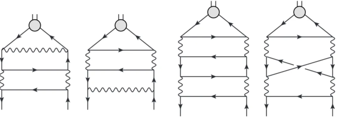
Figure 3. The 1/n²order diagrams for the singlet currents.

For the 1/n

²

order anomalous dimension γ

_s⁽²⁾

we found γ

_s⁽²⁾

= γ

_s⁽¹⁾

η

₁

ψ(s+µ−2)−ψ(µ+1)+ 2µ−1

µ−1 [ψ(2µ−1)+ψ(−µ)−ψ(µ)−ψ(1)]

− µ(µ−1)

2(s+µ−1)(s+µ−2)

1− 1

s+µ−1 − 1 s+µ−2

+ µ

(µ−1)(s+µ−2) + 1 2

µ µ−1

− µ

µ−1 [ψ(µ)−ψ(s+µ−2)]

− η

₁²

2 µ

²

1− (µ−1)

²

(s+µ−1)(s+µ−2)

R

s

(µ) , (3.12) where R

_s

(µ) is (cf. with eq. (5.11) in [31])

R

s

(µ) =

Z 1

0

dα (1 − α)

^µ−2 Z 1

0

dβ (1 − β)

^µ−2

(1 − α − β )

^s−1

. (3.13) The last term in (3.12), the only contribution which can not be expressed in terms of Euler’s ψ-function, comes entirely from the diagram in the r.h.s. in figure

2. Finally, as a

simple consistency check one can verify that γ

⁽²⁾

(s = 1) ≡ γ

_s=1⁽²⁾

+ η

₂

= 0.

3.2 Singlet currents at 1/n

²

In order to find the anomalous dimensions of the singlet currents at 1/n

²

order one has to calculate diagrams shown in figure

3

and the diagrams with all possible self-energy and vertex insertions to the rightmost diagram in figure

1. The calculation does not bring

about any troubles and can be easily performed with the help of the standard methods, see ref. [56] for a review.

3.2.1 Anomalous dimensions

The anomalous dimensions of the singlet currents with odd spins are equal to those of non-singlet ones. The scaling dimensions of the currents with even spins can be written as

∆

s

= 2µ + s − 2 + 1 n

η

1

+ γ

_s⁽¹⁾

+ ∆γ

_s⁽¹⁾

+ 1 n

²

η

2

+ γ

⁽²⁾_s

+ ∆γ

⁽²⁾_s

+ O

1

n

³

. (3.14)

JHEP01(2017)132

The indices η

1,2

are defined in eqs. (2.21), (2.22), γ

s⁽¹⁾

, γ

s⁽²⁾

— in eqs. (3.11), (3.12), respec- tively, and ∆γ

_s⁽¹⁾

is the additional shift in (3.5b) for the singlet currents at order 1/n:

∆γ

_s⁽¹⁾

= −η

₁

µΓ(2µ − 1)Γ(s + 1)

(µ + s − 2)(µ + s − 1)Γ(s + 2µ − 3) . (3.15) For the second order correction ∆γ

_s⁽²⁾

we found

∆γ

_s⁽²⁾

= η

1

∆γ

_s⁽¹⁾ (

2 2µ−1 µ−1

ψ(2µ−1)+ψ(−µ)−ψ(µ)−ψ(1)

− 1 2

3

ψ(2µ+s−3)−ψ(µ+s−2)+ψ(2−µ)−ψ(2)

+ψ(s)−ψ(1)+ 1 s+2µ−3 +ψ(µ+s−2)−ψ(µ)+4 2µ−1

µ(µ−1) +1

− µ µ−1

ψ(s)+ψ(2µ−2+s)−2ψ(s+µ−1)+ψ(2−µ)+ψ(µ)−2ψ(1)

)

− 1

2 γ

_s⁽¹⁾

∆γ

_s⁽¹⁾

(

µ+s−2

(µ−1)(2µ+s−3) +2

−1+ 1

µ+s−1 + 1 µ+s−2

+ψ(2µ−3+s)−ψ(µ)+ψ(1−µ)−ψ(s)

)

− 1

2 (∆γ

_s⁽¹⁾

)

²

(

1 s(2µ+s−3) +

−1+ 1

µ+s−1 + 1 µ+s−2

+ψ(2µ+s−3)−ψ(µ)+ψ(2−µ)−ψ(s+1)

− (µ+s−1)(µ+s−2) s(µ−1)(s+2µ−3)

h

ψ(s+2µ−3)+ψ(s+1)−2ψ(s+µ−1)+ψ(µ)−ψ(1)−J

_s

(µ)

i

)

, (3.16) where the function J

s

(µ) is defined as

J

_s

(µ) = Γ(s + µ − 1) s!Γ(µ − 2)

Z 1 0

dα α

^2µ−4+s Z 1

0

dβ β

^µ−2

(1 − β)

^s

1 − αβ . (3.17)

Again, the contribution in the last line in (3.16), which can not be expressed in terms of ψ functions only, is due the rightmost diagram in figure

3. Finally, taking into account that

J

2

(µ) = 1 2

−2S

₁

(µ − 2) + 2S

1

(2µ − 2) + 1 + µ 1 − µ

. (3.18)

one can check that the stress-tensor is conserved, i.e. η

₂

+ γ

⁽²⁾_s=2

+ ∆γ

⁽²⁾_s=2

= 0.

3.3 Conformal spin expansion

Below we check that the anomalous dimensions of singlet and non-singlet currents can be

cast into the form (3.9) when expressed as functions of conformal spin.

JHEP01(2017)132

3.3.1 Conformal spin expansion of non-singlet currents

In order to express the anomalous dimensions in terms of conformal spin we write γ

^±_A

(s) = f

_A^±

(j) = η

1 + f

1

(j)

+ η

²

f

₂^±

(j) , (3.19) where η = η

₁

/n + η

₂

/n

²

+ . . . and j is defined in eq. (3.6). Note that the first term in (3.19) contains both 1/n and 1/n

²

terms. For the functions f

1

and f

₂^±

we get

f

₁

(j) = − µ(µ − 1)

j(j − 1) , (3.20)

f

₂^±

(j) = 1 2

µ

²

− µ + 1

µ(µ − 1) f

₁²

(j) + f

1

(j)

(

2µ − 1 µ − 1

ψ(j) − ψ(µ)

+ µ − 1

2µ − 1

2(µ − 1)

² )

− 1 2 µ

²

1 − (µ − 1)

²

j(j − 1)

R

⁺

(j, µ) ∓ R

⁻

(j, µ)

, (3.21)

where

R

⁻

(j, µ) = Γ

²

(µ − 1) Γ(j + 1 − µ)

Γ(j + µ − 1) , R

⁺

(j, µ) = 1 j

Z 1 0

du u ¯

^j−2₂

F

₁

2 − µ, 1 j + 1

− u

¯ u

. (3.22) The functions R

^±

(j, µ) are related to the function R

_s

(µ) as follows:

R

⁺

(j

_s

, µ) + (−1)

^s−1

R

⁻

(j

_s

, µ) = R

_s

(µ) , (3.23) where j

s

= s + µ − 1. Note also, that in this formulation the spin-one current conservation is equivalent to the constraint f

₂⁻

(µ) = 0.

One can verify that the large j behavior of anomalous dimensions (3.19) agrees with the predictions of refs. [32–34]. It is easy to see for all terms except, may be, R

⁺

(j, µ). For this function one can use the Mellin-Barnes representation for hypergeometric function to get asymptotic expansion

R

⁺

(j, µ) = 1 2πi

Z i∞

−i∞

dt Γ(2 − µ + t)Γ

²

(1 + t)Γ(−t)Γ(j − t − 1) Γ(2 − µ)Γ(j + t + 1) '

j→∞

X

k≥0

c

_k

Γ(j − k − 1) Γ(j + k + 1) ,

(3.24) with c

k

= (−1)

^k

k!Γ(2 − µ + k)/Γ(2 − µ).

3.3.2 Conformal spin expansion of singlet currents We can rewrite the answer for the singlet current in the form

γ (s) = f (j) = η

1 + f

₁

(j) + ∆f

₁

(j) + η

²

f

₂⁺

(j) + ∆f

₂

(j)

+ O(1/n

³

) , (3.25) where j = s+µ−1+γ (s)/2, the functions f

1

(j), f

₂⁺

(j) are defined by eqs. (3.20), (3.21) and

∆f

₁

(j) = f

₁

(j) Γ(2µ − 1) µ − 1

Γ(j − µ + 2)

Γ(j + µ − 2) . (3.26)

JHEP01(2017)132

For the function ∆f

₂

(j) we obtained

∆f

₂

(j) = ∆f

₁

(j)

(

−

h

ψ(j) − ψ(µ)

i

− 2µ − 1 µ − 1

Ψ(j, µ) − Ψ(µ, µ)

− 1 2

ψ(2 − µ) − ψ(µ)

− 1 2

1

j(j − 1) + (2µ − 3)(3µ − 1)

2(µ − 1)(j − µ + 1)(j + µ − 2) + 1

(µ − 1)

²

+ 1

2µ(µ − 1) − 1

− 1 2 f

₁

(j)

ψ(1 − µ) − ψ(µ − 1) − 2 + 2µ − 3

(j − µ + 1)(j + µ − 2)

− 1

2 ∆f

1

(j) ψ(2 − µ) − ψ(µ) − 1 + 1

(j − µ + 1)(j + µ − 2)

− j(j − 1)

(µ − 1)(j − µ + 1)(j − 2 + µ)

h

Ψ(j, µ) + ψ(µ) − ψ(1) − J(j, µ)

i

!)

, (3.27) where

Ψ(j, µ) = ψ(j − 2 + µ) + ψ(j + 2 − µ) − 2ψ(j) (3.28) and J(j, µ) is an analytic continuation of the function J

_s

(µ), defined in (3.17), to non-integer spins: J(j

s

, µ) = J

s

(µ), for j

s

= s + µ − 1:

J(j, µ) = Γ(j)

Γ(µ − 2)Γ(j + 2 − µ)(j + µ − 2)

Z 1

0

duu

^µ−2

u ¯

^j−µ₂

F

₁

1, 1 j + µ − 1

− u

¯ u

= 1

Γ(µ − 2)

Γ(j − 2 + µ) Γ(j + 2 − µ)

1 2πi

Z i∞

−i∞

dt Γ

²

(t + 1)Γ(µ + t)Γ(−t) Γ(j − µ + 1 − t) Γ(j + µ − 1 + t) .

(3.29) It can be checked that f

₂⁺

(j) + ∆f

2

(j) vanishes for j = µ + 1, so that the anomalous dimension of the energy-momentum tensor, γ (s = 2) = 0, as it should be. Next, taking into account that for large j

Ψ(j, µ) − Ψ(1 − j, µ) = O(e

^−π|Imj|

) and, as it follows from eq. (3.29),

J(j, µ) '

j→∞

X

n≥0

c

_n

(µ) Γ(j − 2 + µ) Γ(j + 2 − µ)

Γ(j − µ + 1 − n)

Γ(j + µ − 1 + n) (3.30) we conclude that the asymptotic expansion of the function f (j) for large j agrees with the predictions of ref. [34].

3.4 Three dimensions and higher-spin masses

The case of three dimensions is of the most interest. First of all, we give the expression for the index η in d = 3 model

η

1

= 8

3π

²

, η = η

1

n

1 + 28

3n η

1

+ . . .

. (3.31)

JHEP01(2017)132

The full order 1/n

²

anomalous dimension of the non-singlet currents γ

s⁽²⁾

can be simpli- fied to

γ

_s⁽²⁾

= 3η

₁²

4 (4s

²

− 1)

(

3π(−1)

^s

2s

²

− 1

s − 2(24s + 9)

4s

²

− 1 − 48s

(4s

²

− 1)

²

+ 2

− 32 log(2) + 3 2s

²

− 1 s

S

₁

s 2 − 3

4

− S

₁

s

2 − 1 4

− 16S

₁

s − 3 2

)

,

(3.32)

where S

1

(j) ≡ ψ(j + 1) − ψ(1). The singlet anomalous dimensions can also be simplified:

∆γ

_s⁽²⁾

= 3η

₁²

4s

²

− 1

(

− 3 144s

³

+ 92s

²

− 28s − 15 2(4s

²

− 1)

²

+ 11

2 − 8s − 2(14s + 3) log(2)

− 2(7s + 3)S

₁

s − 3 2

+ 2(8s + 3)S

₁

(s − 1) + 3

S

₁

s − 1 2

− S

₁

s − 2 2

)

. (3.33) The conservation of the stress-tensor corresponds to η

2

+ γ

_s=2⁽²⁾

+ ∆γ

_s=2⁽²⁾

= 0.

Using the above results for the anomalous dimensions of the currents in the critical d = 3 GN model one can derive masses of the higher-spin gauge fields (1.2) in the dual AdS

4

model. Plugging the first order anomalous dimensions and (3.32), (3.33) into (1.2) one gets

δm

²_s

= 2

n η

₁

(s − 2) + η

₁²

n

²

1 s(1 + 2s)

(

9

4 π 2s

²

− 1

+ s 224s

³

− 244s

²

+ 88s − 317 3(2s − 1)

+ 9

4 2s

²

− 1

S

1

s 2 − 3

4

− S

1

s 2 − 1

4

+ 9s

S

1

s − 1 2

− S

1

s − 2 2

+ 6s(8s + 3)S

₁

(s − 1) − 6s(7s + 5)S

₁

s − 3 2

− 42s(2s + 1) log(2)

)

.

(3.34) One can see that the graviton remains massless, δm

²_s=2

= 0, as it should be. For large spin the mass-spin dependence for the higher-spin fields, eq. (1.2), can be written in the form

δm

²_s

= 2η(s − 2)

1 + η

κ1

(s) + . . .

. (3.35)

Thus in the leading order this dependence takes the form of linear Regge trajectory with the slope α

⁰

= 1/2η. Note that the same linear mass squared spin dependence holds also in the O(N ) model [47]. The deviation from the linear trajectory,

κ1

(s), is due to the next-to-leading corrections,

κ1

(s) = 1

2s − 1 + 2s − 1 2(s − 2)

f

₂⁺

(s + 1/2) + ∆f

₂

(s + 1/2)

. (3.36)

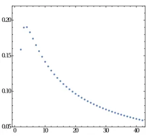
The correction

κ1

(s) is positive for even spins, see figure

4, and vanishes as κ1

(s) =

3

2

ln s/s + . . . for large spin.

JHEP01(2017)132

Figure 4. The functionκ1(2k), eq. (3.36).

4 Summary

We have calculated the 1/n

²

corrections to the scaling dimensions of the (non)singlet higher-spin currents in the GN model. As nontrivial checks we found that the spin-one non-singlet current and the spin-two stress-tensor current are conserved and the asymptotic expansion in terms of conformal spin agrees with the results of refs. [32–34].

In three dimensions the anomalous dimensions can be considerably simplified. Some of the numerical values can be found in appendix

B, which should facilitate comparison

with other methods, e.g. the numerical bootstrap along the lines of [60–62].

Given the anomalous dimensions of the singlet currents we also computed the loop corrections to the masses of higher-spin fields in the four-dimensional higher-spin theory dual to the GN model, known as Type-B. At the leading order the mass spin dependence has the form of a linear Regge trajectory while the next-to-leading correction gives rise to deviation from linearity.

As was observed in [63,

64], there is some diagrammatic dictionary between all the

Feynman-Witten graphs at order 1/N

^k

in the bulk and Feynman graphs at the same order on the CFT side. We note that the graphs of certain topologies present in the bosonic O(N )-model are absent in the Gross-Neveu model since they contain traces of odd number of γ -matrices. This fact indicates that the Type-B higher-spin theory should enjoy some hidden simplicity as compared to the type-A case, which is dual to the bosonic O(N ) model.

Also, as it is clear already from the order 1/n results, there are several contributions to the anomalous dimensions which differ by their large spin asymptotic. It would be interesting to understand this effect from the bulk side.

Acknowledgments

The work of A.M. was supported in part by Deutsche Forschungsgemeinschaft (DFG)

with the grant MO 1801/1-1. The work of E.S. was supported in part by the Russian

Science Foundation grant 14-42-00047 in association with Lebedev Physical Institute and

JHEP01(2017)132

by the DFG Transregional Collaborative Research Centre TRR 33 and the DFG cluster of excellence “Origin and Structure of the Universe”. E.S. would like to thank Munich Institute for Astro- and Particle Physics (MIAPP) of the DFG cluster of excellence “Origin and Structure of the Universe” for the hospitality. E.S. is also grateful to Simone Giombi and Volodya Kirilin for very useful discussions of (Chern-Simons) vector-models.

A Renormalized propagators

For completeness of exposition we give here expressions for the renormalized propagators in the 1/n order assuming that the normalization factor C(∆) is chosen C(∆) = 1. The propagators take the form

D

⁻¹_q

(p) = i

p

p

²

M

²−γ_q

A

_q

(µ) , D

_σ⁻¹

(p) = −nb

⁻¹

(µ)p

^2(µ−1)

p

²

M

²−γ_σ

A

_σ

(µ) , (A.1) where M = 2M , b(µ) is defined by eq. (2.4) and

A

_q

(µ) = 1 + γ

_q

/µ(µ − 1) + O(1/n

²

) , A

σ

(µ) = 1 + γ

σ

ψ(2µ − 1) + ψ(−µ) − ψ(µ) − ψ(1)

+ O(1/n

²

) . (A.2) B Numerical values

Since the formulas for the anomalous dimensions are quite complicated we list below few numerical values in one of the most interesting cases of three dimensions. The order 1/n results are due to [28] and we collect the order 1/n

²

coefficients only. It is worth stressing that we give below the full anomalous dimensions at order 1/n

²

, i.e. η

2

is included. It is convenient to measure the anomalous dimensions in the units of η

₁²

= 64/(9π

⁴

). The spin-one current is always conserved, γ

_A²

(1) = 0, and for few other we find

γ

_A⁽²⁾

(2) = 1104

125 ≈ 8.832 γ

_A⁽²⁾

(3) = 912896

128625 ≈ 7.09734 (B.1) γ

_A⁽²⁾

(4) = 1324432

138915 ≈ 9.53412 γ

_A⁽²⁾

(5) = 154300672

18866925 ≈ 8.17837 . (B.2) The anomalous dimensions of the singlet currents with odd spins are the same as for the non-singlet ones. Below are the full anomalous dimensions at order 1/n

²

for even spins currents. Stress-tensor is conserved, i.e. γ

_S²

(2) = 0, and for a few others we have in the units of η

²₁

γ

_S⁽²⁾

(4) = 16600

3087 ≈ 5.37739 γ

_S⁽²⁾

(6) = 12495584

1816815 ≈ 6.87774 (B.3) γ

_S⁽²⁾

(8) = 145039504

19144125 ≈ 7.57619 γ

_S⁽²⁾

(10) = 133304287652

16712124975 ≈ 7.9765 . (B.4)

Open Access. This article is distributed under the terms of the Creative Commons

Attribution License (CC-BY 4.0), which permits any use, distribution and reproduction in

any medium, provided the original author(s) and source are credited.

JHEP01(2017)132

References

[1] D.J. Gross and A. Neveu,Dynamical Symmetry Breaking in Asymptotically Free Field Theories,Phys. Rev.D 10(1974) 3235 [INSPIRE].

[2] W. Wetzel,Two Loop β-function for the Gross-Neveu Model,Phys. Lett.B 153(1985) 297 [INSPIRE].

[3] J.A. Gracey,Computation of the three loop β-function of the O(N)Gross-Neveu model in minimal subtraction,Nucl. Phys. B 367(1991) 657[INSPIRE].

[4] C. Luperini and P. Rossi,Three loopβ-function(s) and effective potential in the Gross-Neveu model,Annals Phys.212(1991) 371[INSPIRE].

[5] N.A. Kivel, A.S. Stepanenko and A.N. Vasiliev,On calculation of 2 +RG functions in the Gross-Neveu model from large-N expansions of critical exponents,Nucl. Phys. B 424(1994) 619[hep-th/9308073] [INSPIRE].

[6] S.E. Derkachov, N.A. Kivel, A.S. Stepanenko and A.N. Vasiliev,On calculation in1/n expansions of critical exponents in the Gross-Neveu model with the conformal technique, hep-th/9302034[INSPIRE].

[7] J.A. Gracey,Anomalous mass dimension at O(1/N²)in theO(N)Gross-Neveu model,Phys.

Lett.B 297(1992) 293[INSPIRE].

[8] J.A. Gracey,Calculation of exponentη toO(1/N²)in theO(N)Gross-Neveu model,Int. J.

Mod. Phys.A 6(1991) 395[Erratum ibid.A 6 (1991) 2755] [INSPIRE].

[9] A.N. Vasiliev, S.E. Derkachov, N.A. Kivel and A.S. Stepanenko,The 1/n expansion in the Gross-Neveu model: Conformal bootstrap calculation of the indexη in order 1/n³,Theor.

Math. Phys.94(1993) 127[Teor. Mat. Fiz. 94(1993) 179] [INSPIRE].

[10] J.A. Gracey,Computation of critical exponent eta at O(1/N³)in the four Fermi model in arbitrary dimensions,Int. J. Mod. Phys.A 9(1994) 727[hep-th/9306107] [INSPIRE].

[11] J.A. Gracey,Four loop MS-bar mass anomalous dimension in the Gross-Neveu model, Nucl.

Phys.B 802(2008) 330[arXiv:0804.1241] [INSPIRE].

[12] S. El-Showk, M. Paulos, D. Poland, S. Rychkov, D. Simmons-Duffin and A. Vichi, Conformal Field Theories in Fractional Dimensions,Phys. Rev. Lett.112(2014) 141601

[arXiv:1309.5089] [INSPIRE].

[13] S. Rychkov and Z.M. Tan, The-expansion from conformal field theory,J. Phys. A 48 (2015) 29FT01[arXiv:1505.00963] [INSPIRE].

[14] S. Ghosh, R.K. Gupta, K. Jaswin and A.A. Nizami, -Expansion in the Gross-Neveu model from conformal field theory,JHEP 03(2016) 174[arXiv:1510.04887] [INSPIRE].

[15] A. Raju,-Expansion in the Gross-Neveu CFT, JHEP 10 (2016) 097[arXiv:1510.05287]

[INSPIRE].

[16] L.F. Alday and A. Zhiboedov,Conformal Bootstrap With Slightly Broken Higher Spin Symmetry,JHEP 06(2016) 091[arXiv:1506.04659] [INSPIRE].

[17] E.D. Skvortsov,On (Un)Broken Higher-Spin Symmetry in Vector Models, arXiv:1512.05994[INSPIRE].

[18] S. Giombi and V. Kirilin, Anomalous dimensions in CFT with weakly broken higher spin symmetry,JHEP 11(2016) 068[arXiv:1601.01310] [INSPIRE].

[19] K. Diab, L. Fei, S. Giombi, I.R. Klebanov and G. Tarnopolsky, OnCJ andCT in the Gross-Neveu andO(N)models,J. Phys.A 49(2016) 405402[arXiv:1601.07198] [INSPIRE].

JHEP01(2017)132

[20] Y. Hikida,The masses of higher spin fields on AdS₄ and conformal perturbation theory, Phys. Rev.D 94(2016) 026004 [arXiv:1601.01784] [INSPIRE].

[21] P. Dey, A. Kaviraj and K. Sen,More on analytic bootstrap for O(N)models,JHEP 06 (2016) 136[arXiv:1602.04928] [INSPIRE].

[22] K. Nii,Classical equation of motion and Anomalous dimensions at leading order,JHEP 07 (2016) 107[arXiv:1605.08868] [INSPIRE].

[23] R. Gopakumar, A. Kaviraj, K. Sen and A. Sinha, Conformal Bootstrap in Mellin Space, arXiv:1609.00572[INSPIRE].

[24] Y. Hikida and T. Wada, Anomalous dimensions of higher spin currents in large-N CFTs, arXiv:1610.05878[INSPIRE].

[25] P. Basu and C. Krishnan,-expansions near three dimensions from conformal field theory, JHEP 11 (2015) 040[arXiv:1506.06616] [INSPIRE].

[26] V. Bashmakov, M. Bertolini and H. Raj,Broken current anomalous dimensions, conformal manifolds and RG flows,arXiv:1609.09820[INSPIRE].

[27] J.M. Maldacena and A. Zhiboedov,Constraining conformal field theories with a slightly broken higher spin symmetry,Class. Quant. Grav.30(2013) 104003[arXiv:1204.3882]

[INSPIRE].

[28] T. Muta and D.S. Popovic, Anomalous Dimensions of Composite Operators in the Gross-Neveu Model in2 +Dimensions,Prog. Theor. Phys.57(1977) 1705 [INSPIRE].

[29] A.N. Vasiliev and M.Y. Nalimov,Analog of Dimensional Regularization for Calculation of the Renormalization Group Functions in the 1/n Expansion for Arbitrary Dimension of Space,Theor. Math. Phys.55(1983) 423[Teor. Mat. Fiz. 55(1983) 163] [INSPIRE].

[30] A.N. Vasiliev and A.S. Stepanenko,A Method of calculating the critical dimensions of composite operators in the massless nonlinearσ-model,Theor. Math. Phys.94(1993) 471 [Teor. Mat. Fiz.95(1993) 160] [INSPIRE].

[31] S.E. Derkachov and A.N. Manashov, The Simple scheme for the calculation of the anomalous dimensions of composite operators in the 1/N expansion,Nucl. Phys. B 522(1998) 301 [hep-th/9710015] [INSPIRE].

[32] B. Basso and G.P. Korchemsky, Anomalous dimensions of high-spin operators beyond the leading order,Nucl. Phys. B 775(2007) 1[hep-th/0612247] [INSPIRE].

[33] L.F. Alday, A. Bissi and T. Lukowski, Large spin systematics in CFT,JHEP 11(2015) 101 [arXiv:1502.07707] [INSPIRE].

[34] L.F. Alday and A. Zhiboedov,An Algebraic Approach to the Analytic Bootstrap, arXiv:1510.08091[INSPIRE].

[35] J.M. Maldacena, The Large-N limit of superconformal field theories and supergravity,Int. J.

Theor. Phys.38(1999) 1113[Adv. Theor. Math. Phys. 2(1998) 231] [hep-th/9711200]

[INSPIRE].

[36] S.S. Gubser, I.R. Klebanov and A.M. Polyakov, Gauge theory correlators from noncritical string theory,Phys. Lett.B 428(1998) 105[hep-th/9802109] [INSPIRE].

[37] E. Witten,Anti-de Sitter space and holography,Adv. Theor. Math. Phys. 2(1998) 253 [hep-th/9802150] [INSPIRE].

[38] I.R. Klebanov and A.M. Polyakov, AdS dual of the critical O(N)vector model,Phys. Lett.B 550(2002) 213[hep-th/0210114] [INSPIRE].

JHEP01(2017)132

[39] R.G. Leigh and A.C. Petkou,Holography of theN = 1higher spin theory onAdS₄,JHEP 06 (2003) 011[hep-th/0304217] [INSPIRE].

[40] E. Sezgin and P. Sundell, Holography in 4D (super) higher spin theories and a test via cubic scalar couplings,JHEP 07(2005) 044[hep-th/0305040] [INSPIRE].

[41] S. Giombi and X. Yin,Higher Spin Gauge Theory and Holography: The Three-Point Functions,JHEP 09(2010) 115[arXiv:0912.3462] [INSPIRE].

[42] S. Giombi and I.R. Klebanov,One Loop Tests of Higher Spin AdS/CFT,JHEP 12(2013) 068[arXiv:1308.2337] [INSPIRE].

[43] S. Giombi, I.R. Klebanov and A.A. Tseytlin, Partition Functions and Casimir Energies in Higher SpinAdS_d+1/CF T_d,Phys. Rev.D 90(2014) 024048 [arXiv:1402.5396] [INSPIRE].

[44] S. Giombi, S. Minwalla, S. Prakash, S.P. Trivedi, S.R. Wadia and X. Yin, Chern-Simons Theory with Vector Fermion Matter, Eur. Phys. J.C 72 (2012) 2112[arXiv:1110.4386]

[INSPIRE].

[45] O. Aharony, G. Gur-Ari and R. Yacoby, D= 3Bosonic Vector Models Coupled to Chern-Simons Gauge Theories,JHEP 03(2012) 037[arXiv:1110.4382] [INSPIRE].

[46] L. Girardello, M. Porrati and A. Zaffaroni, 3-D interacting CFTs and generalized Higgs phenomenon in higher spin theories on AdS,Phys. Lett.B 561(2003) 289[hep-th/0212181]

[INSPIRE].

[47] W. R¨uhl,The Masses of gauge fields in higher spin field theory on AdS4,Phys. Lett.B 605 (2005) 413[hep-th/0409252] [INSPIRE].

[48] R. Manvelyan, K. Mkrtchyan and W. R¨uhl,Ultraviolet behaviour of higher spin gauge field propagators and one loop mass renormalization,Nucl. Phys. B 803(2008) 405

[arXiv:0804.1211] [INSPIRE].

[49] A.N. Vasiliev and M.I. Vyazovsky,Proof of the absence of multiplicative renormalizability of the Gross-Neveu model in the dimensional regularization d= 2 + 2, Theor. Math. Phys.113 (1997) 1277[Teor. Mat. Fiz. 113(1997) 85] [INSPIRE].

[50] A.N. Vasiliev, M.I. Vyazovsky, S.E. Derkachov and N.A. Kivel, On the equivalence of renormalizations in standard and dimensional regularizations of2D four-fermion

interactions,Theor. Math. Phys.107(1996) 441[Teor. Mat. Fiz.107(1996) 27] [INSPIRE].

[51] A.N. Vasiliev, M.I. Vyazovsky, S.E. Derkachov and N.A. Kivel, Three-loop calculation of the anomalous field dimension in the full four-fermionU(N)-symmetric model,Teor. Mat. Fiz.

107N3(1996) 359 [Theor. Math. Phys.107(1996) 710] [INSPIRE].

[52] J.A. Gracey, T. Luthe and Y. Schr¨oder, Four loop renormalization of the Gross-Neveu model, Phys. Rev.D 94(2016) 125028 [arXiv:1609.05071] [INSPIRE].

[53] J. Zinn-Justin, Four fermion interaction near four-dimensions,Nucl. Phys.B 367(1991) 105[INSPIRE].

[54] A.N. Vasiliev, Y.M. Pismak and Y.R. Khonkonen, 1/N Expansion: Calculation of the Exponentsη and Nu in the Order1/N² for Arbitrary Number of Dimensions, Theor. Math.

Phys.47 (1981) 465[Teor. Mat. Fiz.47(1981) 291] [INSPIRE].

[55] A.N. Vasiliev, Y.M. Pismak and Y.R. Khonkonen, 1/n expansion: calculation of the exponent eta in the order1/n³ by the conformal bootstrap method,Theor. Math. Phys.50(1982) 127 [Teor. Mat. Fiz.50(1982) 195] [INSPIRE].

[56] A.N. Vasilev, The field theoretic renormalization group in critical behavior theory and stochastic dynamics, Chapman & Hall/CRC, Boca Raton U.S.A. (2004) [INSPIRE].

JHEP01(2017)132

[57] S.E. Derkachov and A.N. Manashov,Critical dimensions of composite operators in the nonlinearσ-model,Theor. Math. Phys.116(1998) 1034[Teor. Mat. Fiz. 116(1998) 379]

[INSPIRE].

[58] M. Ciuchini, S.E. Derkachov, J.A. Gracey and A.N. Manashov,Quark mass anomalous dimension atO(1/N_f²) in QCD, Phys. Lett.B 458(1999) 117[hep-ph/9903410] [INSPIRE].

[59] M. Ciuchini, S.E. Derkachov, J.A. Gracey and A.N. Manashov,Computation of quark mass anomalous dimension atO(1/N_f²)in quantum chromodynamics, Nucl. Phys.B 579(2000) 56[hep-ph/9912221] [INSPIRE].

[60] S. El-Showk, M.F. Paulos, D. Poland, S. Rychkov, D. Simmons-Duffin and A. Vichi, Solving the3D Ising Model with the Conformal Bootstrap,Phys. Rev.D 86(2012) 025022

[arXiv:1203.6064] [INSPIRE].

[61] L. Iliesiu, F. Kos, D. Poland, S.S. Pufu, D. Simmons-Duffin and R. Yacoby, Bootstrapping 3D Fermions,JHEP 03(2016) 120[arXiv:1508.00012] [INSPIRE].

[62] S. El-Showk, M.F. Paulos, D. Poland, S. Rychkov, D. Simmons-Duffin and A. Vichi, Solving the3dIsing Model with the Conformal Bootstrap II.c-Minimization and Precise Critical Exponents,J. Stat. Phys.157(2014) 869[arXiv:1403.4545] [INSPIRE].

[63] S. Giombi and X. Yin,On Higher Spin Gauge Theory and the Critical O(N)Model,Phys.

Rev.D 85(2012) 086005[arXiv:1105.4011] [INSPIRE].

[64] X. Bekaert, E. Joung and J. Mourad, Comments on higher-spin holography,Fortsch. Phys.

60(2012) 882[arXiv:1202.0543] [INSPIRE].