Two-loop evolution equations for light-ray operators

arXiv:1404.0863v1 [hep-ph] 3 Apr 2014

Two-loop evolution equations for light-ray operators

V.M. Braun

¹

and A.N. Manashov

^1,2

1 Institut f¨ur Theoretische Physik, Universit¨at Regensburg, D-93040 Regensburg, Germany

2 Department of Theoretical Physics, St.-Petersburg University, 199034, St.-Petersburg, Russia

Abstract

QCD in non-integer d= 4−2ǫ space-time dimensions possesses a nontrivial critical point and enjoys exact scale and conformal invariance. This symmetry imposes non- trivial restrictions on the form of the renormalization group equations for composite operators in physical (integer) dimensions and allows to reconstruct full kernels from their eigenvalues (anomalous dimensions). We use this technique to derive two-loop evolution equations for flavor-nonsinglet quark-antiquark light-ray operators that en- code the scale dependence of generalized hadron parton distributions and light-cone distribution amplitudes in the most compact form.

1.

Studies of hard exclusive reactions contribute significantly to the research program at all major existing and planned accelerator facilities. The relevant nonperturbative input in such processes involves operator matrix elements between states with different momenta, dubbed generalized parton distributions (GPDs), or vacuum-to-hadron matrix elements re- lated to light-front hadron wave functions at small transverse separations, the distribution amplitudes (DAs). Scale dependence of these distributions is governed by the renormalization group (RG) equations for the corresponding (nonlocal) operators and has to be calculated to a sufficiently high order in perturbation theory in order to make the QCD description of exclu- sive reactions fully quantitative. At present, the evolution equations for GPDs (and DAs) are known to the two-loop accuracy [1–3], one order less compared to the corresponding “inclu- sive” distributions that involve forward matrix elements [4, 5] and closing this gap is desirable.

The direct calculation is very challenging, and also finding a suitable representation for the results may become a problem as the two-loop evolution equations for GPDs are already very cumbersome.

It has been known for some time [6] that conformal symmetry of the QCD Lagrangian allows one to restore full evolution kernels at given order of perturbation theory from the spectrum of anomalous dimensions at the same order, and the calculation of the special conformal anomaly at one order less. This result was used to calculate the complete two-loop mixing matrix for twist-two operators in QCD [7–9], and derive the two-loop evolution kernels in momentum space for the GPDs [1–3]. In Ref. [10] we have suggested an alternative technique, the difference being that instead of studying conformal symmetry breaking in the physical theory [7–9] we make

use of theexact conformal symmetry of a modified theory – QCD ind= 4−2ǫ dimensions at critical coupling. Exact conformal symmetry allows one to use algebraic group-theory methods to resolve the constraints on the operator mixing and also suggests the optimal representation for the results in terms of light-ray operators. In this way a delicate procedure of the restoration of the evolution kernels from the results for local operators is completely avoided. We expect that these features will become increasingly advantageous in higher orders.

This modified approach was illustrated in [10] on several examples to the two- and three- loop accuracy for scalar theories. Application to gauge theories, in particular QCD, involves several subtleties that are considered in this work. The main new result are the two-loop evo- lution equations for flavor-nonsinglet quark-antiquark light-ray operators that encode the scale dependence of generalized hadron parton distributions and light-cone distribution amplitudes in the most compact form.

2.

Before going over to technical details, let us first describe the general structure of the approach and the results on a more qualitative level. In order to make use of the (approximate) conformal symmetry of QCD it is natural to use a coordinate-space representation in which the symmetry transformations have a simple form [11]. The relevant objects are light-ray operators that can be understood as generating functions for the renormalized leading-twist local operators:

[O](x;z1, z2) ≡ [¯q(x+z1n)/nq(x+z2n)] ≡ X

m,k

z^m₁ z^k₂

m!k![(D_n^mq)(x)/¯ n(D^k_nq)(x)]. (1) Hereq(x) is a quark field, the Wilson line is implied between the quark fields on the light-cone, Dn =nµD^µ is a covariant derivative, n^µ is an auxiliary light-like vector, n² = 0, that ensures symmetrization and subtraction of traces of local operators. The square brackets [. . .] stand for the renormalization using dimensional regularization and MS subtraction. We will tacitly assume that the quark and antiquark have different flavor so that there is no mixing with gluon operators. In most situations the overall coordinatex^µis irrelevant and can be put to zero; we will often abbreviateO(z1, z2)≡ O(0;z1, z2).

Light-ray operators satisfy a renormalization-group equation of the form [12]

M∂M +β(g)∂g+H

[O(z1, z2)] = 0, (2)

where H is an integral operator acting on the light-cone coordinates of the fields. It can be written as

H[O](z1, z2) = Z 1

0

dα Z 1

0

dβ h(α, β) [O](z^α₁₂, z₂₁^β), (3) where

z₁₂^α ≡z1α¯+z2α , α¯ = 1−α , (4) and h(α, β) is a certain weight function (kernel).

One can show, see e.g. [10], that the powers [O](z₁, z₂)7→(z₁−z₂)^N are eigenfunctions of the evolution operatorH, and the corresponding eigenvalues

γN = Z

dαdβ h(α, β)(1−α−β)^N−1 (5)

are nothing else as the anomalous dimensions of local operators of spinN (withN−1 deriva- tives).

In general the functionh(α, β) is a function of two variables and therefore the knowledge of the anomalous dimensions γN is not sufficient to fix it. However, if the theory is conformally invariant thenHmust commute with the generators of theSL(2) transformations [H, Sα⁽⁰⁾] = 0, where

S₊⁽⁰⁾ =z₁²∂z₁ +z₂²∂z₂ + 2(z1+z2), S₀⁽⁰⁾ =z1∂z₁ +z2∂z₂ + 2, S−⁽⁰⁾ =−∂z₁ −∂z₂. (6) In this case it can be shown that the function h(α, β) (up to trivial terms ∼ δ(α)δ(β) that correspond to the unit operator) takes the form [13]

h(α, β) = ¯h(τ), τ = αβ

¯

αβ¯ (7)

and is effectively a function of one variable τ called the conformal ratio. This function can easily be reconstructed from its moments (5), alias from the anomalous dimensions.

Conformal symmetry of QCD is broken by quantum corrections which implies that the symmetry of the evolution equations is lost at the two-loop level. In other words, writing the evolution kernel as an expansion in the coupling constant

H=asH⁽¹⁾+a²_sH⁽²⁾+. . . 7→ h(α, β) = ash⁽¹⁾(α, β) +a²_sh⁽²⁾(α, β) +. . . , (8) where as = αs/(4π), we expect that h⁽¹⁾(α, β) only depends on the conformal ratio whereas higher-order contributions remain to be nontrivial functions of two variablesα and β.

This prediction is confirmed by the explicit calculation [12]:

H⁽¹⁾f(z1, z2) = 4CF

Z 1 0

dαα¯ α

h2f(z1, z2)−f(z₁₂^α, z2)−f(z1, z₂₁^β)i

− Z 1

0

dα Z α¯

0

dβ f(z^α₁₂, z₂₁^β ) + 1

2f(z1, z2)

. (9)

The corresponding one-loop kernelh⁽¹⁾(α, β) can be written in the following, remarkably simple form [13]

h⁽¹⁾(α, β) =−4CF

δ₊(τ) +θ(1−τ)− 1

2δ(α)δ(β)

, (10)

where the regularizedδ-function,δ+(τ), is defined as Z

dαdβ δ+(τ)f(z₁₂^α, z₂₁^β)≡ Z 1

0

dα Z 1

0

dβ δ(τ)h

f(z₁₂^α, z^β₂₁)−f(z1, z2)i

=− Z 1

0

dαα¯ α

h2f(z1, z2)−f(z₁₂^α, z2)−f(z1, z₂₁^α)i

. (11)

Taking appropriate matrix elements and making a Fourier transformation to the momentum fraction space one can check that the expression in Eq. (10) reproduces all classical leading- order (LO) QCD evolution equations: DGLAP equation for parton distributions, ERBL equa- tion for the meson light-cone DAs, and the general evolution equation for GPDs.

The two-loop kernel h⁽²⁾(α, β) contains contributions of two color structures and a term proportional to the QCD beta function,

h⁽²⁾(α, β) = 8C_F²h⁽²⁾₁ (α, β) + 4CFCAh⁽²⁾₂ (α, β) + 4b0CFh⁽²⁾₃ (α, β). (12) Let us explain how it can be calculated. The idea of Ref. [10] is to consider a modified theory, QCD in non-integerd= 4−2ǫ dimensions. In this theory theβ-function has the form

β(a) = M∂Ma= 2a

−ǫ−b₀a+O(a²)

, b₀ = 11

3 Nc −2

3nf, (13) and for a large number of flavorsnf there exists a critical coupling a^∗_s =α^∗_s/(4π)∼ǫsuch that β(a^∗_s) = 0. The theory thus enjoys exact scale invariance [14,15] and one can argue (see below) that full conformal invariance is also present.¹ As a consequence, the renormalization group equations are exactly conformally invariant: the evolution kernels commute with the generators of the conformal group. The generators are, however, modified by quantum corrections as compared to their canonical expressions (6):

Sα =S_α⁽⁰⁾+a^∗_sS_α⁽¹⁾+ (a^∗_s)²S_α⁽²⁾+. . . (14) One can show that

S⁻=S−⁽⁰⁾,

S0 =S₀⁽⁰⁾−ǫ+1

2H(a^∗_s), H(a^∗_s) =a^∗_sH⁽¹⁾+. . . S+=S₊⁽⁰⁾+ (z1+z2)

−ǫ+ 1

2a^∗_sH⁽¹⁾

+a^∗_s(z1−z2)∆++O(ǫ²), (15) where

∆₊[O](z₁, z₂) =−2CF

Z 1 0

dαα¯

α + lnαh

[O](z₁₂^α, z₂)−[O](z₁, z₂₁^α)i

(16) i.e. the generatorS⁻ is not modified, the deformation ofS₀ can be calculated exactly in terms of the evolution operator (to all orders in perturbation theory) [10], whereas the deformation ofS+ is nontrivial and has to be calculated explicitly order by order, to the required accuracy.

The one-loop expression shown in (15), (16) is derived below, it is a new result. From the pure technical point of view, this calculation replaces evaluation of the conformal anomaly in the theory with broken symmetry in integer dimensions via the conformal Ward identities (CWI) in the approach due to D. M¨uller [6].

1Formally the gauge-fixed QCD Lagrangian contains two charges, the coupling and the gauge parameter.

The correspondingβ-function,βξ =M ∂Mξ, vanishes in the Landau gauge,ξ= 0, so thatallGreen functions are scale-invariant at the critical point in this gauge;βξ also drops out of the RG equations for the correlation functions of gauge-invariant operators.

Conformal symmetry of the modified QCD at the critical coupling implies that the gener- ators (15) satisfy the usual SL(2) commutation relations

[S0, S^±] =±S^±, [S+, S⁻] = 2S0. (17) Expanding them in powers of the coupling a^∗_s one obtains a nested set of commutator rela- tions [10]

[S₊⁽⁰⁾,H⁽¹⁾] = 0,

[S₊⁽⁰⁾,H⁽²⁾] = [H⁽¹⁾,∆S₊⁽¹⁾],

[S₊⁽⁰⁾,H⁽³⁾] = [H⁽¹⁾,∆S₊⁽²⁾] + [H⁽²⁾,∆S₊⁽¹⁾], (18) etc. Note that the commutator of the canonical generator S₊⁽⁰⁾ with the evolution kernel at order k on the l.h.s. of each equation is given in terms of the evolution kernels H^(k) and the corrections to the generators ∆S₊^(m) at one order less, m≤k−1. The commutation relations Eq. (18) can be viewed as, essentially, inhomogeneous first-order differential equations on the evolution kernels. Their solution determines H^(k) up to an SL(2)-invariant term (solution of a homogeneous equation [H^(k)inv, Sα⁽⁰⁾] = 0), which can, again, be restored from the spectrum of the anomalous dimensions. This procedure is described in detail for scalar theories in Ref. [10].

Last but not least, in MS-like schemes the evolution kernels (anomalous dimensions) do not depend on the space-time dimension by construction. Indeed, the renormalization Z factors relating the renormalized and bare light-ray operators [O](z₁, z2) = ZO(z₁, z2) are given by the expansion

Z= 1 + X∞

j=1

ǫ^−j X∞

k=j

a^k_sZjk, (19)

whereZjk have the integral representation similar to (3) in terms of functions of two variables, Zjk(α, β) that do not depend on ǫ. Thus, eliminating the ǫ-dependence of the expressions derived in thed-dimensional (conformal) theory for the critical coupling by the expansion ǫ=

−b₀a^∗_s+O(a^∗_s²) allows one to restore the evolution kernels for the theory in integer dimensions for arbitrary couplinga^∗_s →as; this rewriting is simple and exact to all orders.

3.

The statement of conformal invariance of QCD in d dimensions at the critical cou- pling is not trivial. It is believed that “physically reasonable” scale-invariant theories are also conformally invariant, see Ref. [16] for a discussion, however, to the best of our knowledge there is no proof of this statement for d > 2 dimensions (but there are no counterexamples as well). In non-gauge theories conformal invariance for the Green functions of basic fields can be checked in perturbative expansions [17]. In gauge theories conformal invariance does not hold for the correlators of basic fields and can be expected only for the Green functions of gauge-invariant operators. For local composite operators a proof of conformal invariance is based on the analysis of pair counterterms for the product of the trace of energy-momentum tensor and local operators [18]. This analysis is beyond the scope of this Letter; it becomes rather complicated in gauge theories due to mixing of gauge invariant operators with BRST variations and equation of motion (EOM) operators [19].

A short comment may, nevertheless, be relevant. Let ON be a gauge-invariant multiplica- tively renormalizable operator

M∂M +β(a)∂a+γN(a)

[ON] = 0, (20)

where γN(a) is the anomalous dimension. As a consequence, it possesses a certain (critical) dimension for the fine-tuned value of the coupling (critical point)a =a^∗,β(a^∗) = 0:

i[D,[ON](x)] =

x∂x+ ∆^∗_N

[ON](x), (21)

whereDis the operator of dilatations, ∆N is the canonical dimension of the operatorON, and

∆^∗_N = ∆N +γ_N^∗ is the scaling dimension, γ_N^∗ =γN(a^∗).

The statement that [ON](x) becomes a conformal operator at the critical point, as widely expected, means that action of the generator of special conformal transformations on this operator takes the form

i[K^µ,[O_N](x)] =

2x^µ(x∂)−x²∂^µ+ 2∆^∗_Nx^µ+ 2x^ν

n^µ ∂

∂n^ν −nν

∂

∂nµ

[O_N](x). (22) Equivalently, a correlation function of such operators at the critical point must satisfy the Ward identity

K_x^µ₁ +. . .+K_x^µn

h[O1](x1). . .[On](xn)i= 0, (23) where it is assumed that all space-time points xi are different. Calculating the l.h.s. in perturbation theory (see Ref. [18]) and making use of the dilatation Ward identity produces the expression of the form

K_x^µ₁ +. . .+K_x^µn

h[O₁](x₁). . .[On](xn)i= XN

i=1

D[O₁](x₁). . .Oe_i^µ(xi). . .[On](xn)E

, (24) whereOei(xi) are local operator insertions that involve several contributions: EOM operators, operators representing a BRST variation of another operator, and gauge-invariant operators.

The first two can be neglected as the do not contribute to the correlation function (assuming xj 6= xk, for all j 6= k). The last ones can further be expanded in terms of gauge invariant operators [O_iq^µ](xi) with a certain critical dimension,

Oe^µ_i(xi) =X

q

cq(a)[O_iq^µ](xi).

Dilatation invariance implies that the both sides of Eq. (24) must have the same scaling di- mension at the critical point. Note that application ofK^µ lowers the scaling dimension of an operator by one. As a consequence, for each contribution on the r.h.s., eithercq(a^∗) vanishes, or the scaling dimensions of [O^µ_iq] and [O_i] must differ by one, dimO_iq^µ = dimO_i−1, to all orders of perturbation theory. If such operators do not exist, then all coefficient cq(a) have to vanish at the critical point that implies conformal invariance Eq. (23). For the leading-twist operators

that are subject of this Letter, absence of operators with the same anomalous dimension and the canonical dimension less by one is easy to verify. For the general case, it would be quite unexpected that two different operators have the same anomalous dimension if they are not related by some exact symmetry, although existence of such pairs cannot be excluded.

4.

The correction ∆S+, S+ =S₊⁽⁰⁾+ ∆S+, to the generator of special conformal transfor- mations at the critical point in QCD inddimensions (in the light-ray operator representation) can be derived from the analysis of CWIs for suitable correlation functions. The standard pro- cedure is to consider the Green functions of twist-two operators with quark fields, see Refs. [3,7]

(for d = 4), which are not gauge invariant that complicates the analysis. This difficulty can be avoided by considering, instead, the correlator of two light-ray operators that depend on different auxiliary vectorsn and ¯n:

G(x, z, w) =

[O⁽ⁿ⁾](0, z) [O^(¯n)](x, w)

= N⁻¹ Z

DΦe^−SR(Φ)[O⁽ⁿ⁾](0, z) [O^(¯n)](x, w), (25) where Φ ≡ {A, q,q, c,¯ c}¯ is the set of fundamental fields, z ≡ {z1, z2}, w ≡ {w1, w2} and we assume that the auxiliary light-like vectors are normalized as (n·n) = 1.¯

The QCD Lagrangian in d = 4−2ǫ dimensional Euclidean space-time in covariant gauge has the form²

L = ¯q(∂/−ig /A)q+ 1

4F_µν^a F^a,µν +∂µ¯c^a(D^µc)^a+ 1

2ξ(∂A^a)². (26) The renormalized action SR is obtained from (26) by the replacement

Φ→Φ0 =ZΦΦ, g →g0 =M^ǫZgg , ξ→ξ0 =Zξξ , (27) i.e. SR(Φ, g, ξ) = S(Φ0, g0, ξ0). Note that we do not send ǫ → 0 in the action and the renor- malized correlation functions so that they explicitly depend onǫ.

The form of the CWI is simpler for the special choice (n·x) = (¯n·x) = 0 that we accept for this calculation. For the local conformal operators defined with respect to the ¯n vector, O^(¯_Nⁿ⁾(x), cf. [11], it follows from from Eq. (22) that

i[(¯nK),O^(¯_Nⁿ⁾(x)] = −x²(¯n∂x)O_N^(¯n)(x). (28) Going over to the light-ray operators one obtains, therefore

i[(¯nK),O^(¯n)(x, w)] =−x²(¯n∂x)O^(¯n)(x, w). (29) Thus conformal invariance of the correlation function (25) at the critical point implies the constraint

i 2

[(¯nK),O⁽ⁿ⁾](0, z)O^(¯n)(x, w) +O⁽ⁿ⁾(0, z) (¯nK),O^(¯n)(x, w)]

=

=

S₊^(z)−1

2x²(¯n∂x)

G(x, z, w) = 0, (30)

2Our notation follows closely Ref. [20]

where the superscriptS₊^(z) reminds that it is a differential operator acting onz1, z2 coordinates.

Explicit expression forS₊^(z) can be derived from the CWI 0 = −

δ+SR[O⁽ⁿ⁾](z) [O^(¯n)](x, w) +

δ+[O⁽ⁿ⁾](z) [O^(¯n)](x, w) +

[O⁽ⁿ⁾](z)δ+[O^(¯n)](x, w) , (31) where [O](z1, z2) ≡ [O](x = 0;z1, z2), that follows from invariance of the correlation func- tion (25) under a change of variables Φ7→Φ +δ+Φ in the path integral,

δ+q(x) = ¯n^µ

2xµ(x∂)−x²∂µ+ 2∆qxµ

q(x) + 1

2[γµ, /x]q(x) , δ+Aρ(x) = ¯n^µ

2xµ(x∂)−x²∂µ+ 2∆Axµ

Aρ(x) + 2gµρ(xA)−2xρAµ(x) , δ+c(x) = ¯n^µ

2xµ(x∂)−x²∂µ+ 2∆cxµ

c(x),

δ+¯c(x) = ¯n^µ

2xµ(x∂)−x²∂µ+ 2∆¯cxµ

¯c(x). (32)

The choice of the parameters ∆Φ is a matter of convenience. They can be taken, e.g., equal to the canonical dimensions of the fields in d space-time dimensions, as in [10]. For QCD a different choice proves to be more convenient: ∆q = 3/2−ǫ, ∆A = 1, ∆c_¯= 2 and ∆c = 0. In this case the quark part of the Lagrangian is invariant and variation of the action takes the form

δ+SR= 4ǫ Z

d^dx(x¯n)(LA+Lξ+Lghost) + 2(d−2)¯n^µ Z

d^dx

Z_c²¯c Dµc− 1

ξAµ(∂A)

. (33) The reason for choosing different scaling dimensions for the ghost and anti-ghost fields is that in this case the last term∼(d−2) that does not vanish in four dimensions is a BRST variation [1]

Z_c²c¯^aDµc^a−1

ξA^a_µ(∂A^a)

=δBRST(¯c^aA^a_µ). (34) Hence, it does not contribute to the variation of (25).

In this work we are interested in the one-loop correction to the generator S+. To this accuracy, obviously, the ghost Lagrangian Lghost and gluon self-interaction do not contribute i.e. we have to keep terms quadratic in gluon fields only. One obtains after some algebra

δ+SR=−2ǫ Z

d^dx

(x¯n)A^a_αK^αβA^a_β+ 1 + 1

ξ

(¯nA^a)(∂A^a)

+. . . , (35) where the ellipses stands for the terms that are irrelevant at one loop order and

K^αβ =g^αβ∂²−∂^α∂^β

1−1 ξ

(36) is nothing but the inverse gluon propagator (with a minus sign). Moreover, as follows from Eq. (34), the last term∼(¯nA)(∂A) can be written as a combination of the BRST variation and

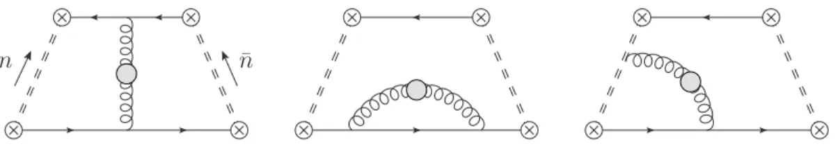
Figure 1: One-loop diagrams contributing to the correlation function of two light-ray operators with an insertion of δ+SR (grey blobs). Wilson lines between the quark fields are shown by the dashed double lines.

the ghost term, so that it does not contribute to the one-loop accuracy as well. Thus, to our ac- curacy, the insertion ofδ+SR generates an effective vertex insertion −2ǫ(¯nx)A^a_α(x)K^αβA^a_β(x) in a gluon line in one loop diagrams:

x

y

= 2ǫn¯·(x+y)

x

y

(37)

Feynman diagrams contributing to the correlation function

δ+SR[O⁽ⁿ⁾](z)[O^(¯n)](x, w) on the r.h.s. of the CWI (31) are shown in Fig. 1. Since the δ₊SR insertion brings the factor ǫg², we only need the divergent parts. The calculation is very easy. For definiteness let us choose the Feynman gauge,ξ = 1, and consider the first diagram in Fig. 1 as an example. This diagram, potentially, has two divergent subgraphs — left and right — but the right one does not contribute due to our choice (¯n, x) = 0, taking into account that the operator O^(¯n)(x, w) only involves quark fields along the line ¯n^µ. Thanks to (37) the divergent part of the left subgraph coincides up to a prefactor 2ǫ(¯n, y+y^′), with the corresponding counterterm for the operatorO⁽ⁿ⁾(z1, z2), which is known from Ref. [12]. One obtains for this contribution

(n¯n)αs

π CFH⁽⁺⁾(z1+z2)G⁽⁰⁾(x, z, w), (38) whereG⁽⁰⁾(x, z, w) is the tree-level correlation function (25) and the integral operatorH⁽⁺⁾ is defined as follows:

H⁽⁺⁾f(z1, z2) = Z 1

0

dα Z α¯

0

dβ f(z₁₂^α, z₂₁^β ). (39) The other diagrams in Fig. 1, similarly, are written in terms of contributions of the correspond- ing counterterms toO⁽ⁿ⁾(z₁, z₂) decorated by multiplicative factors. For the sum of all terms one obtains

δ+SR[O⁽ⁿ⁾](0, z) [O^(¯n)](x, w)

= (40)

= (nn)¯ αs

π CF

h− {Hb₁, z1} − {Hb₂, z2}+

H⁽⁺⁾− 1 2

(z1+z2) +z12Hb^′i

G⁽⁰⁾(x, z, w) +O(ǫ),

where{∗,∗} stands for an anticommutator and b

H₁f(z1, z2) = Z 1

0

dαα¯ α

f(z1, z2)−f(z₁₂^α, z2) , Hb₂f(z₁, z₂) =

Z 1 0

dαα¯ α

f(z₁, z₂)−f(z₁, z₂₁^α) , Hb^′f(z1, z2) =

Z 1 0

dαlnα

f(z₁₂^α, z2)−f(z1, z₂₁^α)

. (41)

The one-loop evolution operatorH⁽¹⁾ in Eq. (8) is written in terms of these kernels as H⁽¹⁾ = 4CF

hHb₁+Hb₂− H⁽⁺⁾+ 1 2

i. (42)

This representation is equivalent to the one in Eq. (10) and, as it is easy to show,H⁽¹⁾commutes withS₊⁽⁰⁾.

Next, we have to consider the second contribution on the r.h.s. of the CWI (31), which involves the conformal variation of [O^(¯n)](x, w),

δ₊[O^(¯n)](x, w) =Zδ₊O^(¯n)(x, w) =Z −x²(¯n∂x)

O^(¯n)(x, w) = −x²(¯n∂x)[O^(¯n)](x, w), (43) and, finally, the third contribution

δ₊[O⁽ⁿ⁾](z) = 2(nn)¯ Zδ₊[O⁽ⁿ⁾](z) = 2(nn)¯ Z

S₊⁽⁰⁾−ǫ(z₁ +z₂)

Z⁻¹[O⁽ⁿ⁾](z)

= 2(nn)¯

S₊⁽⁰⁾−ǫ(z1+z2)− as

2[H⁽¹⁾, z1+z2)]

[O⁽ⁿ⁾](z). (44) This last contribution is discussed in detail in Ref. [10] where the chain of equations in (44) is explained. Collecting all terms we obtain the result quoted in Eq. (15). Note that this expression is different from the corresponding result in scalar field theories,

S₊=S₊⁽⁰⁾+ (z₁+z₂)

−ǫ+1

2a^∗H⁽¹⁾ , see Ref. [10].

5.

We proceed to calculate the NLO evolution kernels (12) making use of the commu- tator relation [S₊⁽⁰⁾,H⁽²⁾] = [H⁽¹⁾,∆S₊⁽¹⁾], Eq. (18). Note that ∆S₊⁽¹⁾ (15) contains terms in b0

and CF 3. Hence the commutator [∆S₊⁽¹⁾,H⁽¹⁾] contains two color structures, b0CF and C_F², respectively. It follows that the kernelCFCAh⁽²⁾₂ (α, β) (12) satisfies the homogeneous equation [S₊⁽⁰⁾,H⁽²⁾2 ] = 0, alias it is SL(2)-invariant and can be written as a function of the conformal ratio,h⁽²⁾₂ (α, β) = h⁽²⁾₂ (τ).

Calculating the commutator we obtain after some algebra

[∆S₊⁽¹⁾,H⁽¹⁾] = 8C_F² A1+ 4CF b0A3, (45)

3To the one-loop accuracy one can replaceǫ= (4−d/2) by −b0a^∗s.

whereA1 and A3 are integral operators of the form Aif(z1, z2) = z12

Z 1 0

dα Ai(α)

f(z₁₂^α, z2)−f(z1, z₂₁^α) +z12

Z 1 0

dα Z α¯

0

dβ Bi(α, β)f(z₁₂^α, z₂₁^β ), with

A1(α) = lnαln ¯α− 3

2α¯−(2−α) lnα+2 +α

α α¯ln ¯α , B1(α, β) = (β−α)h3

2 −ln(1−α−β)i

−αlnα+βlnβ+ 1

αln ¯α− 1 β ln ¯β ,

A3(α) = ¯α , B3(α, β) =α−β . (46)

The simplest way to calculate the evolution kernelsh⁽²⁾₁ , h⁽²⁾₃ is to try the following ansatz:

h⁽²⁾_k (α, β) =−δ+(τ)h

φk(α) +φk(β)i

+ϕk(α, β) +ckδ(α)δ(β). (47) Calculating the commutator [S₊⁽⁰⁾,H⁽²⁾] one obtains first-order differential equations on the functionsφk, ϕk (the terms in ck drop out from the commutator)

¯

α²∂αφk(α) = −Ak(α), αα∂¯ α−ββ∂¯ β

ϕk(α, β) =Bk(α, β), (48)

where∂α =d/dα, etc. The solutions can be chosen as φ1(α) =−ln ¯α

3

2 −ln ¯α+1 + ¯α

¯ α lnα

, φ3(α) = ln ¯α , ϕ1(α, β) =−θ(1−τ)h1

2ln²(1−α−β) + 1

2ln²α¯+1

2ln²β¯−lnαln ¯α−lnβln ¯β

− 1

2lnα− 1

2lnβ+ α¯

αln ¯α+β¯ β ln ¯βi

,

ϕ3(α, β) =−ln(1−α−β)θ(1−τ). (49)

They are defined up to arbitrary solutions of the corresponding homogeneous equations: a constant forφ1,3(α) and a function of the conformal ratio forϕ1,3(α, β). These missing pieces and also the complete kernel h⁽²⁾₂ (τ) can be fixed from the known spectrum of the two-loop anomalous dimensions.

The well-known decomposition

γ_N⁽²⁾ =m⁺_N + (−1)^N−1m⁻_N, (50) where m^±_N can be extended to analytic functions m^±(N) with poles at negative real axis, corresponds for light-ray operators to the decomposition in integration regions where the quark and the antiquark retain their ordering on the light cone or are interchanged

h(τ) =θ(1−τ)h⁺(τ) +θ(τ −1)h⁻(τ⁻¹), (51)

corresponding to α+β <1 and α+β >1, respectively. The equations m^±(N) =

Z 1 0

dα Z α¯

0

dβ h^±(τ) (1−α−β)^N−1 (52) can be inverted as

h^±(τ) = 1 2πi

Z +i∞

−i∞

dN(2N + 1)m^±(N)PN

1 +τ 1−τ

, (53)

where PN is the Legendre function. The integration goes along the imaginary axis such that all poles ofm^±(N) lie to the left of the integration contour. In practice it turns out to be more efficient to start from a certain “educated guess” for the kernels, calculate the moments and find the coefficients.

The final result reads h⁽²⁾₁ (α, β) =−δ+(τ)

φ1(α) +φ1(β)

+ϕ1(α, β) +θ(¯τ)

2 Li2(τ) + ln²τ¯+ lnτ− 1 + ¯τ τ ln ¯τ

+θ(−¯τ)

ln²(−¯τ /τ)− 2

τ ln(−¯τ /τ)

+

−6ζ(3) + 1

3π²+ 21 8

δ(α)δ(β), h⁽²⁾₂ (α, β) = 1

3 π²−4

δ+(τ)−2θ(¯τ)

Li2(τ)−Li2(1) + 1

2ln²τ¯− 1

τ ln ¯τ +5 3

−θ(−¯τ)

ln²(−¯τ /τ)− 2

τ ln(−¯τ /τ)

+

6ζ(3)− 2

3π²+13 6

δ(α)δ(β), h⁽²⁾₃ (α, β) =−δ+(τ)

ln ¯α+ ln ¯β+5 3

−θ(¯τ)

ln(1−α−β) + 11 3

+13

12δ(α)δ(β), (54) where ¯τ = 1−τ, and the functions φ1(α) and ϕ1(α, β) are given in Eq. (49).

6.

Our result for the two-loop evolution of flavor-nonsinglet light-ray operators in Eqs. (12), (54) is equivalent to the corresponding evolution equation for GPDs obtained in Ref. [1] but is more compact and has manifest SL(2) symmetry properties. The latter feature presents the crucial advantage of the light-ray operator (alias position space) representation which makes this technique attractive for higher-order calculations. Exact conformal symmetry of QCD at the critical point proves to be very helpful as it provides one with algebraic group- theory methods to calculate the commutators of integral operators that appear in Eqs. (18).

Evolution equations for GPDs can be obtained from our expressions by a Fourier transforma- tion which is rather straightforward, cf. [21].

Apart from the evolution kernels, another new result is the calculation of the generator of special conformal transformations S+ to the one-loop accuracy, see Eq. (15). The QCD ex- pression differs from the corresponding result in the scalar theory [10] but remains simple. As we have demonstrated, this result can be obtained from the gauge-invariant correlation func- tion of two light-ray operators, thus bypassing the complications due to non-gauge-invariant contributions in the usual approach dealing with Green functions involving fundamental fields.

We expect that the same technique can be used for the flavor-singlet light-ray operators and for the calculation of S+ to the two-loop accuracy, which is the first step towards the NNLO evolution equations. This task, obviously, goes beyond the scope of this Letter.

7. Acknowledgments

We thank D. Mueller for useful discussions. This work was supported by the DFG, grant BR2021/5-2.

References

[1] A. V. Belitsky, A. Freund and D. M¨uller, Nucl. Phys. B 574 (2000) 347.

[2] A. V. Belitsky and D. M¨uller, Nucl. Phys. B537 (1999) 397.

[3] A. V. Belitsky and D. M¨uller, Nucl. Phys. B527 (1998) 207.

[4] S. Moch, J. A. M. Vermaseren and A. Vogt, Nucl. Phys. B 688 (2004) 101.

[5] A. Vogt, S. Moch and J. A. M. Vermaseren, Nucl. Phys. B 691 (2004) 129.

[6] D. M¨uller, Z. Phys. C 49 (1991) 293.

[7] D. M¨uller, Phys. Rev. D 49 (1994) 2525.

[8] D. M¨uller, Phys. Rev. D 58 (1998) 054005.

[9] A. V. Belitsky and D. M¨uller, Phys. Lett. B417 (1998) 129.

[10] V. M. Braun and A. N. Manashov, Eur. Phys. J. C 73 (2013) 2544

[11] V. M. Braun, G. P. Korchemsky and D. Mueller, Prog. Part. Nucl. Phys. 51 (2003) 311.

[12] I. I. Balitsky and V. M. Braun, Nucl. Phys. B 311 (1989) 541.

[13] V. M. Braun, S. E. Derkachov, G. P. Korchemsky and A. N. Manashov, Nucl. Phys. B 553 (1999) 355.

[14] T. Banks and A. Zaks, Nucl. Phys. B196 (1982) 189.

[15] A. Hasenfratz and P. Hasenfratz, Phys. Lett. B297 (1992) 166.

[16] Y. Nakayama, “A lecture note on scale invariance vs conformal invariance,”

arXiv:1302.0884 [hep-th].

[17] S. E. Derkachov, N. A. Kivel, A. S. Stepanenko and A. N. Vasiliev, Theor. Math. Phys.

92, (1992) 1047.

[18] A. N. Vasil’ev, Quantum field renormalization group in the theory of critical behaviour and stohastic dynamics, 774 pages, PNPI Press, Sankt-Petersburg, (1998).

[19] J.C. Collins,Renormalization (CUP, 1984).

[20] M. Ciuchini, S. E. Derkachov, J. A. Gracey and A. N. Manashov, Phys. Lett. B458(1999) 117; Nucl. Phys. B579 (2000) 56.

[21] V. M. Braun, A. N. Manashov and B. Pirnay, Phys. Rev. D80 (2009) 114002 [Erratum- ibid. D 86 (2012) 119902].