Conformal symmetry breaking and evolution equations in Quantum Chromodynamics

and evolution equations in Quantum Chromodynamics

Dissertation zur Erlangung des Doktorgrades der Naturwissenschaften (Dr. rer. nat.) der

naturwissenschaftlichen Fakultät II - Physik der Universität Regensburg

vorgelegt von Matthias Strohmaier

aus Straubing

im Jahr 2018

Prüfungsausschuss: Vorsitzender: Prof. Dr. Karsten Rincke

1. Gutachter: Prof. Dr. Vladimir Braun

2. Gutachter: Prof. Dr. Gunnar Bali

weiterer Prüfer: Prof. Dr. Jascha Repp

sion in the strong coupling constant. The method we use is based on conformal

symmetry arguments. Using Ward identities we derive the conformal symmetry

breaking in QCD in integer dimensions – also known as conformal anomaly – to

two-loop accuracy. This result allows one to define a conformal invariant theory

in d = 4 − 2 dimension by tuning the strong coupling to a certain (critical)

value. The symmetry revealed in that way allows us to solve for the evolution

kernel to the three-loop accuracy. This result is given both in the formulation

of non-local light-ray operators as well as local operators. In the latter case we

present an explicit analytic solution of the NNLO evolution equation on the

example of the pion distribution amplitude.

1 Introduction 11

2 Conformal field theory 15

3 Theory and method 19

3.1 Conformal QCD . . . . 19

3.2 Conformal symmetry of evolution equations . . . . 22

4 Conformal anomaly 27 4.1 Ward identities . . . . 27

4.1.1 Scale Ward identity . . . . 29

4.1.2 Conformal Ward identity . . . . 30

4.2 Perturbative calculation of conformal anomaly . . . . 34

4.2.1 Modified Feynman rules . . . . 34

4.2.2 One-loop anomaly . . . . 36

4.2.3 Two-loop anomaly . . . . 39

5 Evolution equations to NNLO 45 5.1 A short digression on the history of evolution equations . . . . 45

5.2 Details of the method . . . . 46

5.2.1 Similarity transformation . . . . 48

5.2.2 Large-spin expansion and reciprocity . . . . 50

5.3 One-loop evolution kernel . . . . 52

5.4 Two-loop evolution kernel . . . . 52

5.5 Three-loop evolution kernel . . . . 55

5.5.1 Splitting functions . . . . 58

5.5.2 From “x”- to “τ ”-space via Mellin transformation . . . . 62

6 Evolution equation for local operators 65 6.1 Formulation in terms of local operators . . . . 65

6.1.1 Gegenbauer basis operators . . . . 66

6.1.2 Two-loop anomalous dimension matrix . . . . 70

6.1.3 Three-loop anomalous dimension matrix . . . . 71

7 Sample application: Pion distribution amplitude 75 7.1 Definition of the leading-twist pion distribution amplitude . . . . 76

7.2 Perturbative evolution of the pion DA . . . . 79

8 Conclusions 83 8.1 Summary . . . . 83

8.2 Main results . . . . 83

8.3 Outlook . . . . 84

A Collection of renormalization factors 85 B Transformation properties 87 C BRST transformations 89 D Renormalization of gauge invariant operators 91 E Sample Feynman diagram calculation 95 F Results for individual diagrams 97 F.1 Evolution kernel . . . . 97

F.2 Conformal anomaly . . . . 99

G X kernels 103

H Transformation to conformal scheme 107

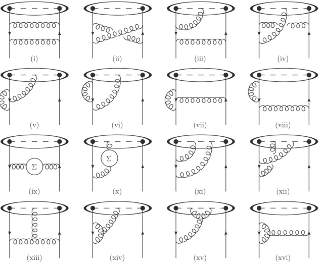
4.1 Feynman diagrams for two-loop evolution kernel . . . . 40

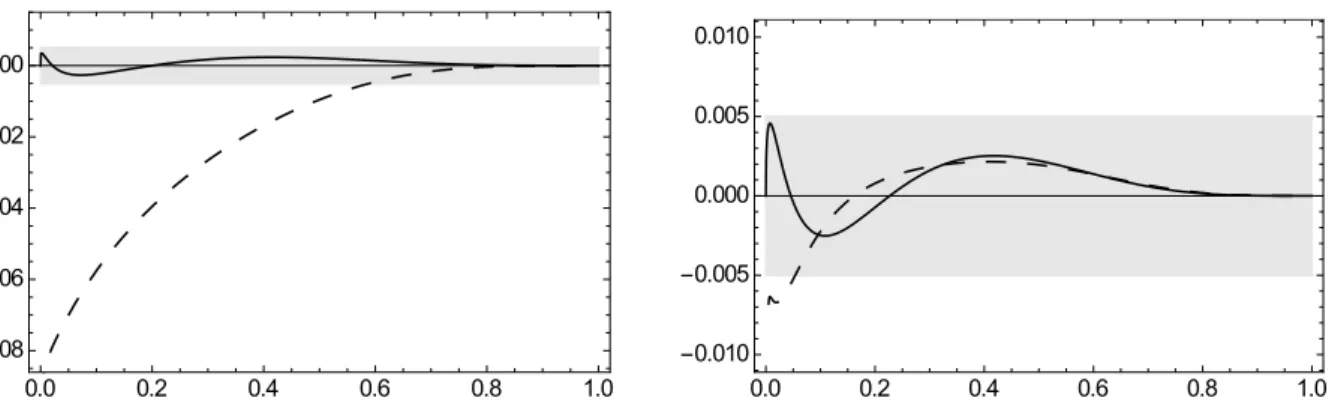
5.1 Error estimate for three-loop evolution kernel . . . . 60

5.2 Invariant kernel functions χ

(τ) and χ

(τ) . . . . 64

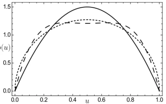
7.1 Models for Pion DA . . . . 79

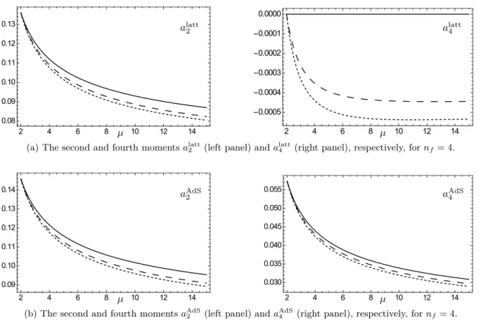
7.2 Scaling of moments of Pion DA . . . . 82

a Lattice moments . . . . 82

b AdS moments . . . . 82

2.1 Conformal transformations and generators . . . . 16

5.1 Fit parameters for δH

(x) . . . . 60

5.2 Analytic parameters for H

(x) . . . . 61

7.1 Moments of Pion DA . . . . 78

Introduction

Half a century has passed since the foundation of Quantum Chromodynamics (QCD) – the theory which

describes the interaction of quarks via exchange of gluons. The concept of quarks was initially introduced

by Gell-Mann and Zweig [1, 2] to avoid limitations due to “fermi’s principle” by additional degrees of

freedom. At that time it was not yet clear whether quarks are actual particles or just some “theoretical

construction”. The first DIS (deep inelastic scattering) experiments at the Stanford Linear Accelerator

(SLAC) [3, 4, 5] encouraged the theoretical picture and gave profound reason to believe that nucleons

are indeed bound states composed of almost free point-like constituents. Shortly later Gell-Mann and

Fritzsch [6] proposed the theory of strong interactions – QCD – which turned out to give a precise

description of the nature. Ever since this time there was an ongoing rally of both experimental and

theoretical activities to gain a better understanding of the strong interaction. Despite all the successes

we are still far from a complete, and in some concerns also detailed, picture. One of the major problems

is that the strong coupling constant α

acquires a peculiar dependence on the energy scale: at high

energies (small distances) it tends to zero, quarks move as free particles and the theory gets trivial. This

phenomenon is known as “asymptotic freedom” [7, 8]. Close to this regime one can construct a series

in the small coupling and truncate this series at a sufficiently high order. However for small energies

(large distances) the coupling grows and perturbation theory cannot be applied. Experiment shows

that quarks and gluons cannot appear as free particles but only as bound states, a phenomenon called

confinement. Among all non-perturbative formulations of the low-energy regime of the theory, Lattice

QCD is the only one based on first principles and certainly the most successful one. Here the space-time

is discretized in a finite volume and the theory is solved numerically. Just as a perturbative approach

fails for large distances, the lattice formulation becomes obviously unreliable for small distances. The

description of most processes requires an understanding of both regimes. The way out is given through

so-called factorization theorems, which allow one to factorize some processes into a hard- (high energy-)

and soft- (low energy-) part. Typically the hard part, often referred to as coefficient functions, depends

on the process under consideration (but not the target particles). The soft part, given in terms of PDFs

(parton distribution functions), TMDs (transverse momentum distributions), GPDs (generalized parton

distributions) or DAs (distributions amplitudes) are process-independent universal functions (but depend

on the particles). Due to their universality they can also be determined by a phenomenological fit to the

data for a certain process and afterwards used for all kind of other processes. The factorization however

introduces an additional unphysical parameter – the factorization scale. In addition the regularization of

both soft- and hard-parts requires the introduction of renormalization scales. The dependence on these

scales is governed by the RGEs (renormalization group equations) or evolution equations. Assuming both hard- and soft-part are exactly known, this ambiguity drops out. However, in reality both are just approximated to some accuracy and therefore some uncertainty in the physical quantities arises. In order to achieve a good precision one needs to keep this uncertainty small.

Studies of hard exclusive reactions contribute significantly to the research program at all major existing and planned accelerator facilities. The relevant non-perturbative input in such processes involves operator matrix elements between states with different momenta, dubbed GPDs, or vacuum-to-hadron matrix elements related to light-front hadron wave functions at small transverse separations, the DAs. The aim of this thesis is to make a step towards the NNLO QCD description of these reactions, which is the calculation of the scale dependence of the relevant parton distributions – GPDs and DAs – to the three-loop accuracy.

This task is more complicated compared to the calculation of the scale dependence of usual parton distributions (DGLAP equations) because the distributions in question involve operator matrix elements sandwiched between states with different momentum. Thus, mixing with the operators containing total derivatives must be taken into account. From the technical point of view, the problem reduces to the calculation of the divergent parts of the relevant three-point functions involving two different external momenta. This is a much harder task as compared to the kinematics of forward scattering where only one external momentum is involved. Whereas in the case of forward kinematics NNLO [9, 10] results are available for quite some time and partial NNNLO results have been published recently [11, 12, 13, 14, 15, 16, 17], in the off-forward case NLO is the current accuracy [18, 19, 20, 21, 22, 23, 24, 25]. Due to the conformal symmetry of QCD at the classical level, the leading order exclusive evolution kernel can be deduced from the inclusive one and the non-trivial off-diagonal part appears at the two-loop level for the first time. It can be shown that this quantity can actually be determined by the conformal symmetry breaking at one-loop. In general it is known [26] that conformal symmetry (breaking) of the QCD Lagrangian allows one to restore full evolution kernels at a given order of perturbation theory from the spectrum of anomalous dimensions – alias the forward kernels – at the same order, and the calculation of the special conformal anomaly at one order less. This result was used to calculate the complete two-loop mixing matrix for twist-two operators in QCD [27, 23, 28], and derive the two-loop evolution kernels in momentum space for the GPDs [29, 24, 25]. In Ref. [30] an alternative technique has been suggested, the difference being that instead of studying conformal symmetry breaking in the physical theory [27, 23, 28] one uses exact conformal symmetry of a modified theory — QCD in d = 4 − 2 dimensions at critical coupling. Exact conformal symmetry considerably simplifies the analysis and also suggests the optimal representation for the results in terms of light-ray operators. It is expected that these features will become increasingly advantageous in higher orders. This modified approach was illustrated in [30]

on several examples to the two- and three-loop accuracy for scalar theories and in [31] to the two-loop accuracy in QCD, reproducing the known results [27, 23, 28].

The outline of the thesis is as follows: The first two chapters 2 and 3 are introductory, we establish the

notion of a conformal field theory (CFT), give a reminder of the QCD Lagrangian and find a connection

between QCD and CFT – conformal QCD at the critical point. We explain the concepts of the running

coupling and evolution equations. Moreover we give a brief overview of the method. In chapter 4 we

study the breakdown of conformal symmetry in integer-dimensional QCD and explicitly restore conformal

symmetry in the modified conformal QCD. As the result we obtain three symmetry generators S

(α

)

which satisfy the conformal algebra to two-loop accuracy. In chapter 5 we use these findings to determine

the evolution equations to the three-loop accuracy. We give explicit results in two different formulations

– in terms of non-local light-ray operators and in terms of local operators. The latter are summarized in

chapter 6, where we first need to establish a convenient conversion from one formulation to the other. In

chapter 7 we apply our results to the evolution of the pion distribution amplitude, that is needed for the

description of hard exclusive reactions involving production of energetic pions:

• the pion transition γ + γ

→ π

and electromagnetic ππγ

form factors

• semi-leptonic and hadronic B-decays B → π`ν

, B → ππ, etc.

• pion electroproduction γ

N → πN and many others.

In chapter 8 we will conclude and give an outline of future progress in this direction. The main text will

be followed by several appendices, which contain technical details and some relevant intermediate results.

Conformal field theory

It is certainly beyond the scope of this thesis to present a comprehensive introduction to conformal field theory. Instead we want to refer to three books, lecture notes and reviews that have been important and in- spiring for studies on that area: Firstly, there is the book by Di Francesco, Mathieu and Senechal [32], that can be seen as the standard book for conformal field theory. Secondly the lecture notes by Ginsparg [33]

give an excellent introduction to the field. Finally, the review by Braun, Korchemsky and Müller [34]

yields an perfect introduction and overview of the application of conformal symmetry to QCD. In the following we will restrict ourselves to a very brief resume of the main ideas from these references with focus on the areas that will be important for this thesis.

Since the dawn of science the concept of symmetries has been appealing to all kind of philosophers and researchers. While in the twentieth-century the idea of symmetries was often used for abstract constructions like gauge-symmetries, the more tangible notion of space-time symmetries is much older and has a long tradition. Even the breakdown of symmetries can be useful, as seen in the theory of phase transitions, critical phenomena [32] and electro-weak interactions. Modern particle physics is based on the concept of (relativistic) quantum field theory, where Poincar´ e-invariance is the fundamental space-time symmetry. A possible extension is given by scale invariance, which is the symmetry under global dilatations. In 1970 Polyakov [35] argued that for physical systems with local interactions it is reasonable to extend scale invariance by dilatations with a local scaling factor, which defines conformal transformations. Moreover, looking for transformations that leave the light-cone invariant, the conformal symmetry group turns out to be the maximal extension of the Poincar´ e-group. More precisely: In a conformal field theory (CFT) the usual Poincar´ e-symmetry of the classical theory is extended by scale transformations x

7→ λx

(λ ∈ R ) and inversion x

7→

. The Poincar´ e group with these new added transformations forms the so-called conformal group. The Lie algebra of the Poincar´ e group is defined by the commutation relations

i[P

, P

] = 0, i[M

, P

] = g

P

− g

P

,

i[M

, M

] = g

M

− g

M

− g

M

+ g

M

, (2.1) and is extended by the following relations that generate the conformal algebra

i[D, P

] = P

, i[D, K

] = −K

,

i[M

, K

] = g

K

− g

K

, i[P

, K

] = −2g

D + 2M

,

i[D, M

] = 0, i[K

, K

] = 0. (2.2)

# finite action generator of inf. action

Translation 4 x

7→ x

+ a

P

= −i∂

Rotation 6 x

7→ ω

x

M

= −i(x

∂

− x

∂

− Σ

)

Dilatation 1 x

7→ λx

D = −i(x · ∂ + ∆

)

SCT 4 x

7→

K

= −i(2x

x · ∂ − x

∂

+ 2∆

x

− 2ix

Σ

)

Table 2.1: The fifteen conformal transformations and their generators, see e.g. Ref. [34]. ∆

is the (canonical) scaling dimension of the field ϕ, for QCD explicit expressions will be given in Eq. (4.7)

For completeness, we collected the transformations and the corresponding generators in table 2.1.

There we introduced the generator of spin rotations Σ

, which takes the following form for scalar, spinor (quark) and vector fields (gluon) fields

Σ

φ = 0, Σ

q = i

2 σ

q, Σ

A

= g

A

− g

A

, (2.3) respectively, where σ

=

[γ

, γ

] is the commutator of two Dirac matrices. As an inversion cannot be generated by an infinitesimal transformation, one usually considers the special conformal transformation (SCT) – the combination of inversion, translation and inversion.

During the past three decades CFT raised a lot of interest in both mathematics and physics and has built an ideal ground for the interplay of these two disciplines in the frame of mathematical physics. The main attention was put on CFT in two dimensions. In this special case the conformal algebra becomes infinite dimensional and thus imposes enough constraints to allow for an exact solution. In particular for string theory great achievements have been made by considering the string surface as a two-dimensional CFT. Despite all these appealing facts one should keep in mind that in dimensions greater than two the conformal algebra reduces to a finite one. Moreover most physical theories involve some natural dimensionful scales, provided by the masses of particles or the renormalization scale, and therefore one cannot expect these theories to feature scale or conformal invariance. Nevertheless it is known [36, 37, 38], that at the fixed point of the renormalization group flow the natural scale of the theory, given by the inverse correlation length, tends to zero and conformal symmetry emerges. This last point makes CFT also appealing for applications to statistical mechanics and condensed matter as it allows for the description of such systems close to the phase transition [39]. In that context the main topic is universality, meaning that several systems share common properties near the critical point and can be grouped into so-called universality classes.

In high-energy physics one most often considers light-cone dominated processes, i.e. ultra-relativistic particles moving close to the light-cone. To describe such kinematics it is appropriate to use light-cone variables

x

= x

n

+ x

n ¯

+ x

, x

= n · x, x

= ¯ n · x, (2.4) where n

= 0 and ¯ n

= 0 define the two light-like directions, for convenience we can assume n · n ¯ = 1. In this picture a hadron is described by partons propagating along a collinear light-like direction

ϕ(x) 7→ ϕ(zn) ≡ ϕ(z), (2.5)

with some real number z. Whenever these kinematics apply for a process, the full conformal group

reduces to a set of three symmetry generators acting non-trivial on the light-cone. These three generators

correspond to the so–called collinear subgroup, SL(2, R ), of the conformal group, which consists of Moebius transformations,

z 7→ z

= az + b

cz + d , where a, b, c, d, z ∈ R , ad − bc = 1. (2.6) Field transformations are given by:

ϕ(z) 7→ T

ϕ(z) = 1

(cz + d)

ϕ( az + b

cz + d ), (2.7)

where the conformal spin j =

(∆ + s) of the field ϕ is given by half of the sum of the spin s and the scaling dimension. The generators for these three transformations are

L

= −iP

, L

= i

2 K

, L

= i

2 (D − M

). (2.8) They obey the SL(2, R ) - algebra

[L

, L

] = ±L

, [L

, L

] = 2L

. (2.9) While the action of the generators on the quantum fields can be easily obtained from the definitions in table 2.1, it turns out to be more convenient to trade them for differential operators acting on the auxiliary variable z

[L

, ϕ(z)] = −∂

ϕ(z) ≡ S

ϕ(z),

[L

, ϕ(z)] = (z

∂

+ 2jz)ϕ(z) ≡ S

ϕ(z),

[L

, ϕ(z)] = (z∂

+ j)ϕ(z) ≡ S

ϕ(z), (2.10) which obey the same algebra

[S

, S

] = ±S

, [S

, S

] = 2S

. (2.11) The n–particle generators are given by the sum of one–particle generators

S

= z

∂

+ 2j

z

+ . . . + z

∂

+ 2j

z

, S

= z

∂

+ j

+ . . . + z

∂

+ j

,

S

= −(∂

+ . . . + ∂

). (2.12)

The quadratic Casimir operator reads

C = S

− S

+ S

S

, (2.13)

and commutes with all three generators

[ C , S

] = 0. (2.14)

Its spectrum, as function of the conformal spin j, is given by C = j(j − 1). The collinear subgroup will

play the central role in our analysis.

Theory and method

3.1 Conformal QCD

We consider massless QCD in the d = 4 − 2 dimensional Euclidean space. The action reads S =

Z d

x n

¯ q / Dq + 1

4 F

F

− ¯ c

∂

(D

c)

+ 1

2ξ (∂

A

)

o

, (3.1)

where D

= ∂

− ig

A

T

is the covariant derivative with T

being the SU (N) generators in the fundamental (adjoint) representation for quarks (ghosts). The field strength tensor is defined as usual

F

= ∂

A

− ∂

A

+ g

f

A

A

. (3.2) Using dimensional regularization the dimension-shift serves as the regulator. For our purpose it will be useful in another context as we will explain later on. The bare coupling constant is g

= gµ

where µ is the scale parameter, introduced by the requirement to leave the action dimensionless. The most natural renormalization scheme in dimensional regularization is the (modified) minimal subtraction (MS)-scheme [40]. The renormalized action is obtained from (3.1) by the replacements

q → Z

q, A → Z

A, c → Z

c, g → Z

g, ξ → Z

ξ, (3.3) where Z

= Z

and the renormalization factors take the form (in (MS)-scheme)

Z = 1 +

∞

X

j=1

∞

X

k=j

z

α

4π

, α

= g

4π . (3.4)

where z

are -independent constants. The anomalous dimensions of the fundamental fields

γ

= µ∂

Z

, (3.5)

are collected in appendix A to the three-loop accuracy. Note that we do not send → 0 in the action

and the renormalized correlation functions so that they explicitly depend on .

Formally the theory has two charges — g and ξ. The corresponding beta-functions are β(a) = µ da

dµ = −2a + ¯ β(a)

β

(ξ, g) = µ dξ

dµ = −2ξγ

, (3.6) where β ¯ = γ

is the anomalous dimension of the coupling constant [8, 7, 41, 42, 43]

β(a) =µ∂ ¯

ln Z

= β

a + β

a

+ β

a

+ O(a

), β

= 11

3 N

− 2

3 n

, β

= 2 3

17C

− 5C

n

− 3C

n

, β

= 2857

54 C

− 1415

54 C

n

+ 79

54 C

n

+ 11

9 C

n

− 205

18 C

C

n

+ C

n

. (3.7) Here and in what follows we use the notation

a = α

4π . (3.8)

At the classical level one can set d = 4 and drop the scale parameter µ in (3.1), which becomes then invariant under conformal and scale transformations. In the interacting theory the introduction of the scale µ, however, explicitly breaks conformal symmetry of the theory. Even in the limit d → 4, which can be taken after a proper renormalization prescription is done, the crucial µ-dependence remains.

The same holds true for all known regularization schemes, e.g. a UV-cutoff or a lattice (where not even Poincar´ e-symmetry is preserved). To recover a conformal field theory and utilize all the powerful tools associated with it we will use the notion of renormalization-group-flow fixed points, which we will introduce in what follows.

It is known [37, 38] that there exists a critical value of the coupling (fixed point), a = a

() such that β (a

) = 0. For a sufficiently large number of flavors n

, the leading order beta-function changes its sign β

< 0. Therefore, in non-integer dimensions d = 4 − 2, we find the critical point

β (a

) = 0, a

= − β

−

β

β

β

−

β

2β

− β

β

β

+ O(

). (3.9) From Eq. (3.6) we see that beta-function associated with the gauge parameter ξ vanishes identically in Landau gauge ξ = 0. As a consequence, Green’s functions of quark and gluon fields in Landau gauge at critical coupling enjoy scale invariance. This can be seen as just a technical trick to consider QCD in d = 4 − 2 as a scale invariant theory. We clearly need to stress that QCD in integer dimensions is not a scale invariant field theory.

So far we just discussed scale invariance. Although Bogoliubov’s famous quote [44] – “There is no

mathematical difference [between scale and conformal symmetry], but when some young people want

to use a fancy word they call it conformal symmetry” – was certainly incorrect in the mathematical

sense, in a physical context it seems to be true that scale invariance usually comes hand in hand with

conformal invariance of the theory: It is believed that “physically reasonable” scale invariant theories are

also conformally invariant, see Ref. [45] for a discussion. In non-gauge theories conformal invariance for

the Green’s functions of basic fields can be checked in perturbative expansions [46]. For local composite

operators a proof of conformal invariance is based on analysis of pair counterterms for the product of

the trace of the energy-momentum tensor and local operators [47]. In gauge theories, including QCD,

conformal invariance does not hold for the correlators of basic fields and can be expected only for the

Green’s functions of gauge-invariant operators. In addition there are extra complications due to mixing

of gauge-invariant operators with BRST variations and equation-of-motion (EOM) operators. We will discuss these issues briefly in what follows.

Renormalization ensures finiteness of the correlation functions of the basic fields that are encoded in the QCD partition function. Correlation functions with an insertion of a composite operator O

– built of n fundamental fields ϕ – possess additional divergences that are removed by the operator renormalization,

[O

] = X

j

Z

O

, (3.10)

where the sum goes over all operators with the same quantum numbers that get mixed; Z

are the renormalization factors that have a similar expansion in inverse powers of as in Eq. (3.4)

Z =

∞

X

i=1

Z

(a)

, Z

(a) =

∞

X

`=i

a

Z

. (3.11) Here and below we use square brackets to denote renormalized composite operators (in a minimal sub- traction scheme).

Renormalized operators satisfy a RG equation with the anomalous dimension matrix (or evolution kernel, in a different representation)

H = −(µ∂

Z ) Z

= 2 X

`

`a

Z

. (3.12)

(up to field renormalization) which has a perturbative expansion with coefficients that in a minimal subtraction scheme do not depend on by construction. As a consequence, the anomalous dimension matrices are exactly the same for QCD in d dimensions that we consider at the intermediate step, and physical QCD in integer dimensions that is our final goal. To be specific, if in d-dimensional QCD at the critical point

µ∂

+ H (a

)

[O] = 0, H (a

) = a

H

+ a

H

+ . . . (3.13) then in d = 4 dimension and for arbitrary coupling

µ∂

+ β(a)∂

+ H (a)

[O] = 0, H (a) = a H

+ a

H

+ . . . (3.14) with the same matrices H

. All what one has to do in going over to the four-dimensional theory is to re-express consistently all occurrences of = (4 − d)/2 in terms of the critical coupling = β

a

+ . . . and replace a

7→ a in the resulting expressions. In other words: there is a hidden symmetry of RG equations in physical QCD in minimal subtraction schemes to all orders in perturbation theory. The requirement of large n

for existence of the critical point is not principal since, staying within perturbation theory, the dependence on n

is polynomial. In this sense the statement above holds for arbitrary number of flavors.

Let us briefly sketch the idea:

• As a first step we go over to a theory in non-integer dimensions, which enjoys exact scale and

conformal invariance at the critical point.

• Using conformal Ward identities we will construct the explicit expressions for the symmetry gener- ators of translations, dilatations and special conformal transformations.

• For QCD in integer dimensions this means we have found three operators that commute with the evolution kernel H and form an SL(2) algebra.

• As we will see below, perturbative expansion of these commutation relations produces a nested set of equations that allow one to determine the non-diagonal parts of the anomalous dimension matrices with a relatively small effort.

Some parts of the construction become simpler and more transparent going over from local operators to the corresponding generating functions that are usually referred to as light-ray operators. This represen- tation is introduced in the next section.

3.2 Conformal symmetry of evolution equations

In this chapter we explain this approach on a more technical level.

In order to make use of the (approximate) conformal symmetry of QCD it is natural to use a coordinate-space representation in which the symmetry transformations have a simple form, see [34] a review. The suitable objects are light-ray operators (see e.g. [48]) which can be understood as generating functions for the renormalized leading-twist local operators. For example

[O

](x; z

, z

) ≡ [¯ q(x + z

n)/ nq(x + z

n)] ≡ X

m,k

z

z

m!k! [(D

q)(x)/ ¯ n(D

q)(x)]. (3.15) Here the Wilson line is assumed between the quark fields on the light-cone, D

= n

D

is a covariant derivative, n

is an auxiliary light-like vector, n

= 0, that ensures symmetrization and subtraction of traces of local operators. The square brackets [. . .] stand for the renormalization using dimensional regularization and MS subtraction. We tacitly assume the quarks to be of different flavor. Unless we denote it differently, the light-ray operator will be aligned in the “plus”-direction n.

The local composite operators defined by the OPE (3.15) do not have simple properties under the transformations defined in table 2.1. Therefore we aim to find operators that can be classified according to the irreducible representations of the SL(2)-algebra. This basis set of operators defines the so-called conformal tower of operators. The highest weight vector of the representation is the lowest operator in the conformal tower and defines the so-called conformal operator Q

(x). It is an eigenfunction of the evolution equation (3.14). There are several equivalent ways to define a conformal operator, upon which the most common reads: The conformal operator must have the same transformation properties as the fundamental field, see. table 2.1. For operators located at the origin x = 0 this just means that it gets annihilated by a special conformal transformation

[L

, Q

(x = 0)] = i

2 K

Q

(x = 0) = 0 (3.16)

The higher operators in the conformal tower are obtained by adding total derivatives

Q

= (n∂)

Q

= [L

, [L

, . . . , [L

, Q

]]] , k = 0, 1, 2, . . . (3.17)

From this definition and the SL(2)-algebra (2.9) one derives the transformation properties

[L

, Q

] = Q

,

[L

, Q

] = (j

+ k)Q

,

[L

, Q

] = −k(2j

+ k − 1)Q

, (3.18) where j

= N + 2 + ¯ β(a

) +

γ

(a

) is the conformal spin of the operator Q

. Obviously all operators Q

in the tower have the same anomalous dimensions γ

. The generators L

act as raising and lowering operators on this representation. The OPE of the light-ray operator (3.15) in terms of this set of basis operators reads

[O](z

, z

) = X

N k

Ψ

(z

, z

)Q

, (3.19)

where the coefficient functions Ψ

(z

, z

) are homogeneous polynomials of degree N + k. To fix the form of these coefficient functions we will trade the generators L

for the differential operators S

a la Eq. (2.10)

[L

, O(z

, z

)] = X

N k

Ψ

(z

, z

) [L

, Q

] = X

N k

S

Ψ

(z

, z

)Q

. (3.20) A simple algebra reveals that the generators S

act as raising and lowering operators on the basis of coefficient functions

S

Ψ

(z

, z

) = −Ψ

(z

, z

), S

Ψ

(z

, z

) = (j

+ k)Ψ

(z

, z

),

S

Ψ

(z

, z

) = (k + 1)(2j

+ k)Ψ

(z

, z

). (3.21) Thus the lowest weight coefficient function is annihilated by translations

S

Ψ

(z

, z

) ≡ S

Ψ

(z

, z

) = 0, (3.22) and therefore must be a shift-invariant function Ψ

(z

, z

) ' (z

− z

)

. The higher weight functions are then obtained by successive action of the conformal generator

Ψ

(z

, z

) ' (S

)

Ψ

(z

, z

) ' (S

)

(z

− z

)

. (3.23) Explicit expressions for the proportionality factors are irrelevant for the moment but will be given later in the text.

Light-ray operators satisfy a renormalization-group equation

(µ∂

+ β(α)∂

+ H ) [O(z

, z

)] = 0, (3.24) where H is an integral operator acting on the light-cone coordinates of the fields. It can be written as

H [O](z

, z

) = Z

0

dα Z

0

dβh(α, β)[O](z

, z

) + 2γ

[O](z

, z

), (3.25)

1Here we still assumex= 0. The action of the symmetry generators on operators at arbitrary space-time pointsxtakes more involved form and is derived in appendix B

where γ

is the quark anomalous dimension,

z

= ¯ αz

+ αz

, α ¯ = 1 − α (3.26)

and h(α, β) is a certain weight function, often also associated with the term “evolution kernel”. The spectrum of the evolution kernel

H (z

− z

)

= (γ

+ 2γ

)(z

− z

)

, (3.27) is given by the well-known forward anomalous dimensions [9, 11, 12, 13, 14, 15, 16, 17]

γ

= Z

dαdβ h(α, β)(1 − α − β )

. (3.28)

In general the function h(α, β) is a function of two variables and therefore the knowledge of the eigenvalues – that are the anomalous dimensions γ

– is not sufficient to fix it. However, to leading order the theory is conformally invariant and H must commute with the generators of the SL(2) transformations [ H , S

] = 0, where to the leading order, cf. Eqs. (2.12),

S

= z

∂

+ z

∂

+ 2(z

+ z

) + O(a

) ≡ S

+ O(a

), S

= z

∂

+ z

∂

+ 2 + O(a

) ≡ S

+ O(a

),

S

= − ∂

− ∂

≡ S

. (3.29)

In this case it can be shown that the function h(α, β) takes the form [49]

h(α, β) = ¯ h(τ ), τ = αβ

¯

α β ¯ (3.30)

and is effectively a function of one variable τ called the conformal ratio. This function can easily be reconstructed from its spectrum, alias from the anomalous dimensions.

Conformal symmetry of QCD is broken at the level of quantum corrections which implies that the symmetry of the evolution equations is lost at the two-loop level. In other words, writing the evolution kernel as an expansion in the coupling constant

H = a H

+ a

H

+ . . . ↔ h(α, β) = ah

(α, β) + a

h

(α, β) + . . . (3.31) one expects that h

(α, β) only depends on the conformal ratio whereas higher-order contributions remain to be nontrivial functions of two variables α and β . This prediction can be confirmed by an explicit calculation which reveals that the first-order kernel in QCD has a remarkably simple form

h

(α, β) = C

δ

(τ) − θ(1 − τ ). (3.32) Taking appropriate matrix elements and a Fourier transformation to the momentum space one can check that the expression in Eq. (3.32) reproduces all classical LO QCD evolution equations: DGLAP, ERBL and GPD evolution equation [50, 51, 52]. The idea of Refs. [30, 31] is to consider a modified theory, QCD in non-integer d = 4 − 2 dimensions. This theory enjoys exact scale and conformal invariance [37, 38] at the so–called critical point a

∼ , where β(a

) = 0.

As a consequence, the renormalization group equations are exactly conformally invariant: the evolu- tion kernels commute with the generators of the conformal group:

[ H , S

] = 0. (3.33)

The generators are, however, modified by quantum corrections as compared to their canonical expressions (3.29):

S

= S

+ a

∆S

+ a

∆S

+ . . . (3.34) One can show that [31]

S

= S

, S

= S

− + 1

2 H (a

), S

= S

+ (z

+ z

)

− + a

H

+ a

(z

− z

)∆

+ O(

) (3.35) where

∆

[O](z

, z

) = −C

Z

α ¯

α + ln(α)

[O](z

, z

) − [O](z

, z

)

(3.36) i.e. the generator S

(translation) is not deformed at all, the deformation of S

(dilatation) can be calculated exactly in terms of the evolution kernel (to all orders in perturbation theory), whereas the deformation of S

(special conformal transformation) is nontrivial and has to be calculated explicitly to the required accuracy. It can always be arranged in the form (3.35):

S

= S

+ (z

+ z

)

− + 1 2 H (α

)

+ (z

− z

)∆(α

). (3.37) and the main task will be to calculate the perturbative expansion for

∆(a) = a∆

+ a

∆

+ O(a

). (3.38) From the pure technical point of view, this calculation replaces the evaluation of the conformal anomaly in the theory with broken symmetry in integer dimensions in the approach by D. Müller [27, 23, 28].

In order to derive ∆ one needs to consider Conformal Ward identities (CWI) for the Green’s function of two light-ray operators, one contracted with the auxiliary light-like vector n

, and the other one with

¯ n

:

G(x, z, w) = h[O

](0, z)[O

](x, w)i

= N

Z

Dϕ e

[O

](0, z)[O

](x, w), (3.39) where ϕ ≡ {q, q, A, c, ¯ ¯ c} is the set of all fundamental fields and z = {z

, z

}, w = {w

, w

}.

The statement is the following: conformal symmetry (in the modified theory at the critical point) imposes a constraint on this Green’s function, called CWI. This Ward identity follows from the invariance of the Green’s function under a change of variables ϕ 7→ ϕ + δϕ in the functional integral,

hδ[O

](0, z)[O

](x, w)i + h[O

](0, z)δ[O

](x, w)i

− hδS

[O

](0, z)[O

](x, w)i = 0,

(3.40)

2 both chosen orthogonal tox, i.e.(nx) = (¯nx) = 0and normalized as(¯nn) = 1

where δ corresponds to either a dilatation δ = δ

or a special conformal transformation δ = δ

. This equation is called Conformal Ward identity (CWI) and will be analyzed in great detail later on.

Conformal symmetry of the modified QCD at the critical coupling implies that the generators satisfy the usual SL(2) commutation relations

[S

, S

] = ±S

, (3.41a)

[S

, S

] = 2S

. (3.41b)

Due to the general form (3.35) only the first commutator, i.e. Eq. (3.41a) with a “+” sign, contains non-trivial information. Performing an expansion in powers of the coupling a

one obtains a nested set of commutator relations

[S

, H

] = 0,

[S

, H

] = [ H

, ∆S

],

[S

, H

] = [ H

, ∆S

] + [ H

, ∆S

], .. .

[S

, H

] =

`−1

X

k=1

[ H

, ∆S

]. (3.42)

Note that the commutator of the canonical generator S

with the evolution kernel at order ` on the l.h.s. is given in terms of the evolution kernels H

and the corrections to the generators ∆S

at one order less, k, m ≤ ` − 1. The commutation relations Eq. (3.42) can be viewed as, essentially, inhomogeneous first-order differential equations on the evolution kernels. Their solution determines H

up to an SL(2)-invariant term (solution of a homogeneous equation [ H

, S

] = 0), which can, again, be restored from the spectrum of the anomalous dimensions. Last but not least, in MS-like schemes the evolution kernels (anomalous dimensions) do not depend on the space-time dimension by construction.

Thus the expressions derived in the d-dimensional (conformal) theory for the critical coupling allow one to restore the results for the theory in integer dimensions for arbitrary coupling; this procedure is straightforward and exact to all orders. This approach has been checked in calculations in scalar field theories to the three-loop accuracy [30] and in QCD to two loops [53, 31]. In both cases this technique proves to be very effective and the results can be presented in a compact analytic form.

3This is completely equivalent to the restriction[H, S+] = 0

Conformal anomaly

In this chapter we will calculate the CWI to two-loop accuracy, which determines the corrections to the conformal generators.

4.1 Ward identities

Ward identities (WI) follow from invariance of path integrals under a change of variables, that corresponds to a symmetry transformation. The standard choice is the correlation function of the composite operator in question with a set of fundamental fields. In gauge theories and in particular in QCD it is more convenient to consider the correlation functions of light-ray operators, which are gauge-invariant.

As mentioned above, the operator S

in the light-ray operator representation is defined as the gen- erator of special conformal transformations in the “minus” direction n ¯ acting on the light-ray operator aligned in the “plus” direction n and centered at the origin, x = 0:

L

, [O

](0, z

, z

)

= i 2

nK, ¯ [O

](0, z

, z

)

= S

O

(0, z

, z

). (4.1) (Here we display explicitly the dependence on the auxiliary vector n in the definition of the light-ray operator). On the other hand, taking the transformation and operator along the “minus” direction ¯ n and choosing x such that (x · n) = 0 ¯ one gets, see Eq. (B.11)

L

, [O

](x, z

, z

)

= i 2

nK, ¯ [O

](x, z

, z

)

= − 1

2 x

(¯ n∂

) O

(x, z

, z

). (4.2) Let us consider the Green’s function of these two light-ray operators [O]

(0, z) and [O]

(x, w) that are separated by a transverse distance (x · n) = (x · n) = 0: ¯

G(x; z, w) = D

[O

](0, z) [O

](x, w) E

. (4.3)

Here we use the shorthand notation z = {z

, z

}, w = {w

, w

}. The path-integral representation reads G(x; z, w) = N

Z

Dϕ e

[O

](0, z) [O

](x, w). (4.4)

Here N is a normalization factor, S

(ϕ) is the renormalized QCD action, ϕ = {A, q, q, c, ¯ ¯ c} and the functional integration goes over all fields.

Let us perform the infinitesimal field transformations from table 2.1 in the path-integral ϕ 7→ ϕ + λδ

ϕ, δ

ϕ = x∂

+ ∆

ϕ(x), (4.5)

ϕ 7→ ϕ + a

δ

ϕ, δ

ϕ =

2x

(x∂) − x

∂

+ 2∆

x

− 2Σ

x

ϕ(x), (4.6) corresponding to the dilatation and special conformal transformations, respectively. Ghost fields are scalars, thus they transform under spin rotations as follows, see Eq. (2.3),

Σ

c = Σ

¯ c = 0.

The definition for the scaling dimensions ∆

of the fundamental fields is a matter of taste, a convenient choice is [24]:

∆

= 3

2 − , ∆

= 1, ∆

= 0, ∆

= 2 − 2. (4.7)

The choice ∆

= 1 ensures that the gluonic field strength tensor transforms covariantly under conformal transformations

δ

F

= h

2x

(x∂) − x

∂

+ 4x

− 2Σ

x

i

F

, (4.8)

and the reason for ∆

= 0 is that for this choice a covariant derivative of the ghost field D

c(x) transforms as a vector field of dimension one, i.e. in the same way as the gluon field A

.

Demanding invariance of the Green’s function G(x; z, w) in the path-integral representation under conformal variations implies the Ward identities

D δ[O

](0, z) [O

](x, w) E + D

[O

](0, z) δ[O

](x, w) E

− D

δS

[O

](0, z) [O

](x, w) E

= 0, (4.9)

where δ = δ

or δ = δ

= ¯ n

δ

for either scale or conformal transformations, (4.5) and (4.6). The variation of the QCD action δS

takes in both cases the following form

δ

S

= Z

d

x N (x), δ

S

=

Z

d

x 2x

N (x) − (d − 2)∂

B

(x)

, (4.10)

where

N (x) = 2 L

= 2 1

4 Z

F

+ 1 2ξ (∂A)

, B

(x) = Z

cD ¯

c − 1

ξ A

(∂A). (4.11)

It is known [46] that for QFTs with certain properties

one finds

2x

δ

L

= δ

L

, (4.12)

and accordingly scale invariance implies conformal invariance of the theory. For QCD, however, these properties are spoiled by an extra term ∼ ∂

B

(x) in the conformal variation that does not vanish in the limit → 0. Hence the QCD action is not invariant under conformal transformations even for integer d = 4 dimensions. Luckily, since we only consider the correlator of gauge-invariant operators one can show that this operator B

(x) does not give any contributions, as it can be written as a BRST variation of ¯ c

A

[24], see Appendix C.

On the other hand, conformal invariance of QCD at the critical point implies the constraint D [L

, [O

](0, z)] [O

](x, w) + [O

](0, z) [L

, [O

](x, w)] E

=

=

S

− 1

2 x

(¯ n∂

)

G(x; z, w) = 0, (4.13)

where the superscript S

reminds that it is a differential operator acting on the z

, z

coordinates.

Equation (4.13) can be seen as a definition for what is meant by conformal symmetry at the critical point. By comparing the equations (4.9) and (4.13) one finds an expression for the exact conformal generator S

in the conformal theory.

In what follows we analyze the structure of the Ward identities (4.9) in detail.

4.1.1 Scale Ward identity

We start our analysis with the scale WI (SWI). First, the variation of the renormalized light-ray operator is given by

δ

[O

](x, z) = Zδ

O

(x, z) =

x∂

+ X

i=1,2

z

∂

+ 3 − 2

[O

](x, z). (4.14)

Here we used Zδ

Z

= δ

, which is true since the term

x∂

+ P

i=1,2

z

∂

+ 3 − 2

counts the canonical dimension of the operators and renormalization mixes only operators with the same canonical dimension. Thus we derive for Eq. (4.9)

x∂

+ X

i=1,2

(z

∂

+ w

∂

) + 6 − 4

G(x; z, w) = D

δ

S

[O

](0, z) [O

](x, w) E

. (4.15)

The l.h.s. is nothing else than the logarithmic derivative w.r.t. scale parameter P

i

(∆

+ x

· ∂

) = µ∂

, and making use of the evolution equation (3.14) we arrive at the final form for the SWI

D

δ

S

[O

](0, z) [O

](x, w) E

= −

β (a)∂

+ H

(a) + H

(a)

G(x; z, w). (4.16)

1i. Interaction contains only fields without derivatives ii. Translation- and rotation-invariance

iii. Kinetic terms in action are scale and conformally invariant

This results reflects the common wisdom that the SWI is nothing else than a renormalization group equation. Another way to understand this equation is to compare it with the standard way to derive the RGE. In the usual approach one calculates the Green’s function and takes the 1/ pole part, while in the SWI one considers an insertion δ

S

∼ R

d

xL

and takes the finite part. The two methods differ by additional insertions in gluon propagators, three- and four-gluon vertices, and gauge-fixing terms.

Hence both Green’s functions must be equal up to combinatorial factors. This factor is given by the number of gluon-lines and vertices of each diagram and is just equal to the number of loops of each diagram minus one , i.e. the eigenvalue of the operator a∂

− 1.

4.1.2 Conformal Ward identity

The two terms on the l.h.s. of the conformal Ward identity (CWI), Eq. (4.9), correspond to the variation of the light-ray operators. The first one can be expressed in terms of S

,

δ

[O

](0, z) = Zδ

O

(0, z) = 2ZS

O

(0, z) = 2ZS

Z

[O

(0, z)], (4.17) where S

= S

− (z

+ z

), the term −(z

+ z

) is due to the modification of the quark scaling dimension ∆

=

− , cf. (4.7).

The conformal variation of the second light-ray operator retains its leading order form (for our choice (x · n) = 0) ¯

δ

[O

](x, w) = −x

(¯ n · ∂

)[O

](x, w). (4.18) Thus the CWI takes the form

2ZS

Z

− x

(¯ n · ∂

)

G(x; z, w) = D

δ

S

[O

](0, z) [O

](x, w) E

= 2 Z

d

y (¯ n · y) D

N (y)[O

](0, z) [O

](x, w) E

, (4.19) where in the second line we have discarded the term due to the BRST operator ∂

B

(4.10) as it does not contribute to gauge-invariant correlation functions. Comparison with eq. (4.13) yields the following constraint for the full conformal generator

S

G(x; z, w) = Z S

Z

G(x; z, w) + Z

d

y (¯ n · y) D

N (y)[O

](0, z) [O

](x, w) E

(4.20)

The product Z S

Z

can be expanded (see Ref. [30]) as Z S

Z

= S

− 1

2 Z

0

du u

h

H (u), z

+ z

i + . . .

= S

− 1

2 a [ H

, z

+ z

] − 1

4 a

[ H

, z

+ z

] + O(a

) + . . . (4.21)

where the ellipses denote singular 1/ terms. An explicit expression for the singular contributions is

not needed since they must cancel in the sum of both terms on the right hand side of eq. (4.20). The

remaining task is to determine the contribution due to the variation of the action. This will be done in

a perturbative expansion by evaluation of the corresponding Feynman diagrams.

First we want to point out that correlation functions of elementary fields with the operator insertion N (x) must be finite. Hence we can express the operator insertion in terms of finite operators. The result reads [54, 25, 24, 34, 55, 47]

N (y) = − β (a) a

L

− (γ

+ γ

)E

− X

ϕ6=A

γ

E

+ γ

ξ [(∂A)

] + r

∂

E

+ r

∂

[B

], (4.22) where E

= [E

] are EOM operators, E

= ϕ(y)

δS

/δϕ(y)

and ∂

E

= E

− E

= ∂

[¯ cD

c − ∂

c c]. ¯ The derivation of this expression can be found in Appendix D. The method explained there, however, does not work to constrain the constants r

(a, ξ) and r

(a, ξ). As we will see this issue will not cause any trouble, since the corresponding operators do not contribute to the CWI (4.20).

Let us analyze the individual terms in Eq. (4.22) separately.

i. The EOM contributions are simple, as they give rise to contact terms that can be evaluated using integration by parts in the path-integral

D E

(y)O

O

E

= D

ϕ(y) δO

δϕ(y) O

E + D

O

ϕ(y) δO

δϕ(y) E

. (4.23)

The contribution due to the quark EOM reads D

δ

S

[O

] [O

] E

Eq

= −2γ

(z

+ z

)G(x; z, w) + singular terms. (4.24) As it was mentioned we will drop singular terms since they must cancel in the end. The ghost EOM operator do not give any contribution to the correlator. In fact this is trivial since

[O

] [O

]

= 0. In the case of gauge fields the situation is more peculiar due to the gauge links in the light-ray operators that produce an infinite amount of gluons. Later on we will find that this term will play a special role.

ii. The last three terms in Eq. (4.22) drop out in the CWI (4.20), as they are ghost EOM and BRST operators, see Eq. (C.6).

iii. The next contribution is due to D

δ

S

[O

] [O

] E

L

= − β(a) a

Z

d

y 2(¯ n · y) D

[L

(y)] [O

] [O

] E

. (4.25)

We want to stress here again that the correlator is accompanied by an factor −

= 2(+ ¯ β). At the critical point β(a

) = 0 we only need to find the divergent part of the correlation function [46, 47].

Since all three operators are renormalized, the divergent part must arise due to pair counterterms from the integration regions y → x and y → 0. Thus we split

D [L] [O

] [O

] E

= Dh

LO

O

iE

− D PCt

LO

[O

] E

− D

[O

] PCt

LO

E

. (4.26)