Investigation of the Charge Symmetry Breaking Reaction dd −→ 4He

Breaking Reaction dd − → ⁴ Heπ ⁰ with the WASA-at-COSY Facility

I ^NAUGURAL - D ISSERTATION

zur

Erlangung des Doktorgrades

der Mathematisch-Naturwissenschaftlichen Fakultät der Universität zu Köln

vorgelegt von

Maria Katarzyna ˙Z UREK aus Chrzanów, Polen

Köln 2017

Prof. Dr. Jan Jolie

Tag der mündlichen Prüfung: 08.11.2016

Abstract

Probing elementary symmetries and symmetry breaking tests our understanding of the theory of strong forces, Quantum Chromodynamics. The presented study concen- trates on the charge symmetry forbidden reaction dd →

Heπ

. The aim is to provide experimental results for comparison with predictions from Chiral Perturbation The- ory (χ

) to study effects induced by quark masses on the hadronic level, e.g., the proton-neutron mass difference.

First calculations showed that in addition to the existing high-precision data from TRIUMF and IUCF, more data are required for a precise determination of the param- eters of χ

. These new data should comprise the measurement of the charge sym- metry forbidden dd →

Heπ

reaction at sufficiently high energy, where the p-wave contribution becomes important. A first measurement with the WASA-at-COSY ex- periment at an excess energy of ε = 60 MeV was performed, but the results did not allow for a decisive interpretation because of limited statistics.

This thesis reports on a second measurement of the dd →

Heπ

reaction at ε = 60 MeV using an improved WASA detector setup aiming at higher statistics. A sample of 336 ± 43 event candidates have been extracted using a data set from an eight-week long beamtime, and total and differential cross sections have been determined. The angular distribution has been described with a function of the form dσ/dΩ = a + b cos

θ

, where θ

is the scattering angle of the pion in the c.m. coordinate system.

The obtained parameters a and b and the total cross section are:

a = 1.75 ± 0.46(stat.)

(syst.)

pb/sr , b = 13.6 ± 2.2(stat.)

(syst.)

pb/sr ,

σ

= 79.1 ± 7.3(stat.)

(syst.) ± 8.1(norm.) ± 2.0(lumi. syst.) pb .

For this experiment a modified detector setup optimized for a time-of-flight mea- surement of the forward going particles has been used. After detector calibration and track reconstruction, signal events have been selected using a chain of cuts and a kine- matic fit. For absolute normalization the integrated luminosity has been obtained us- ing the dd →

Henπ

reaction. The final acceptance correction has been performed using a Monte Carlo signal generator with the measured angular distribution.

The obtained differential cross section indicates the presence of higher partial waves in the final state. A combined interpretation of these results with the other measure- ments of the dd →

Heπ

reaction allowed to determine the square of the magnitude of the p-wave amplitude |C|

= 520 ± 290(stat.)

(syst.)

pb/ sr · (GeV/c)

and the real part of the s − d interference term <{A

A

} = 1670 ± 320(stat.)

(syst.) pb/ sr · (GeV/c)

neglecting any further initial and final state interactions. The result

shows that any theoretical attempt to describe the reaction has to include, in addition

to p-waves, also d-wave contributions.

Zusammenfassung

Die Untersuchung elementarer Symmetrien und ihrer Brechung testet unser Ver- ständnis der Theorie der starken Wechselwirkung, der Quantenchromodynamik. Die vorliegende Doktorarbeit konzentriert sich auf die Reaktion dd →

Heπ

, welche die Ladungssymmetrie verletzt. Das Ziel ist es, die experimentellen Ergebnisse mit den Vorhersagen der chiraler Störungstheorie (χ

) zu vergleichen, um die Effekte von Quarkmassen auf hadronischer Ebene zu untersuchen. Ein Beispiel ist der Einfluß auf die Massendifferenz von Proton und Neutron.

Erste theoretische Rechnungen zeigten, dass zusätzlich zu den bestehenden Hoch- präzisionsdaten von TRIUMF und IUCF weitere Daten für eine genaue Bestimmung der χ

Parameter erforderlich sind. Diese neuen Daten zur Ladungssymmetrie ver- letzenden dd →

Heπ

Reaktion müssen bei ausreichend hoher Energie gemessen werden, da dort die Beiträge von p-Wellen wichtig werden. Eine erste Messung wurde mit dem WASA-at-COSY Experiment bei einer Überschussenergie von ε = 60 MeV durchgeführt, allerdings ließen die Ergebnisse wegen der begrenzten Statistik keine endgültige Interpretation zu.

Diese Dissertation besckäftigt sich mit einer zweiten Messung der Reaktion dd →

4

Heπ

bei ε = 60 MeV mit einem verbesserten Aufbau des WASA-Detektors und dem Ziel einer höheren Statistik. Aus den Daten einer acht Wochen langen Messung wurden 336 ± 43 Eventkandidaten extrahiert. Dabei wurden der totale und differ- entielle Wirkungsquerschnitt bestimmt und die Winkelverteilung mit der Funktion dσ/dΩ = a + b cos

θ

gefittet. Die dadurch erhaltenen Parameter a und b und der totale Wirkungsquerschnitt ergeben sich zu:

a = 1.75 ± 0.46(stat.)

(syst.)

pb/sr , b = 13.6 ± 2.2(stat.)

(syst.)

pb/sr ,

σ

= 79.1 ± 7.3(stat.)

(syst.) ± 8.1(norm.) ± 2.0(lumi. syst.) pb .

Der modifizierte Detektoraufbau, welcher für die Messung verwendet wurde, ist auf die Nutzung der Flugzeit für nach vorne emittierte Teilchen ausgelegt. Die Sig- nalereignisse wurden nach erfolgter Detektorkalibrierung und Spurrekonstruktion mit- tels eines kinematischen Fits und verschiedenen Analyseschnitten ausgewählt. Für die absolute Normalisierung wurde die integrierte Luminosität mit der dd →

Henπ

Reaktion bestimmt. Die endgültige Akzeptanzkorrektur wurde auf der Basis einer Monte-Carlo Simulation durchgeführt, welche die gemessene Winkelverteilung berück- sichtigt.

Der erhaltene differentielle Wirkungsquerschnitt zeigt das Vorhandensein von höhe- ren Partialwellen im Endzustand. Eine gemeinsame Analyse dieser Ergebnisse mit den anderen Messungen der dd →

Heπ

Reaktion erlaubt die Bestimmung des Qua- drats der p-Wellenamplitude |C|

= 520 ± 290(stat.)

(syst.)

pb/ sr · (GeV/c)

und des Realteils des s −d Interferenzterms <{A

A

} = 1670 ± 320(stat.)

(syst.) pb/ sr · (GeV/c)

, ohne die Berücksichtigung von weiteren Anfangs- und Endzus-

tandswechselwirkungen. Das Ergebnis zeigt, dass jede theoretische Beschreibung der

Reaktion zusätzlich zu p-Wellen auch d-Wellen-Beiträge berücksichtigen muss.

Acknowledgements

Undertaking this PhD project has been a truly life-changing experience for me and it would not have been possible to do without the support and guidance that I received from many people.

I would like to express my sincere gratitude to my thesis advisor Prof. Dr. Hans Ströher for making it possible for me to write this thesis at the Forschungszentrum Jülich. Thank you for the support of my research, for your patience, motivation, and immense knowledge in the field of hadron physics. Your guidance helped me con- stantly during research and writing of this thesis. Thank you also for giving me lots of precious advice about how to present my work and the opportunity to participate in workshops and conferences.

I am sincerely grateful to my scientific advisor Dr. Volker Hejny for his excellent guid- ance. Thank you for all the time you spent with me on countless discussions about the analysis, for helping me to understand deeply the experimental and theoretical side of this project, for motivating me to find creative solutions to non-obvious problems, and showing how important carefulness and precision are in experimental work. I am grateful for proofreading this thesis and for all comments on my work, especially these critical ones, because they helped me to improve. I could not imagine having a better mentor. Your experience is really astonishing, I wish every physics collaboration had its own "Volker"!

I would like to thank Prof. Dr. Jan Jolie for reviewing my thesis, as well as Prof. Dr.

Alexander Altland and Prof. Dr. Detlev Gotta for being members of my examination committee.

I am grateful to Prof. Dr. Christoph Hanhart and Dr. Florian Hauenstein for proof- reading this dissertation.

I also want to thank the "charge symmetry breaking team" from Jagiellonian Univer- sity - Prof. Dr. Andrzej Magiera and Dr. Aleksadra Wro ´nska for their help during the experiment, all the discussions and lots of useful advice. Also warm thanks to Dr. Edward Stephenson for wise comments and deep interest in the project.

I would like to express my gratitude to Prof. Dr. Michael Albrow for sharing his passion and enthusiasm for scientific work during our "free-time" project in diffraction physics. I am grateful for your supervision during the internships in Fermilab, when my adventure with particle physics started 6 years ago, and for continuing it when I am at the beginning of my scientific career. I am really lucky I have the opportunity to work with you.

I am grateful to the whole WASA-at-COSY collaboration, especially all people who

were helping me during the beamtime. In total we had 183 eight-hour long shifts to

monitor the experiment. It would not have been possible without you! Big thanks to the "pellet target team": Florian, Kay, Niels and Karsten, for your enormous help and the strength to work even after being called in the middle of the night. I am also grateful to the COSY crew for delivering stable beam and solving all the problems that arose during the beamtime.

I would like to thank all my colleagues from the IKP-1 and IKP-2 institutes for making my workplace more enjoyable every day. Here I would like to especially mention Zara, Lu, Dariusch, Ilhan, Simone, Albrecht, Florian, Andi, Malkhaz, Andro, Irakli, Farha, Michael, Ale, Daniel, Fabian, David, Jenny, Elisabetta, Tobias, Yury, Huagen and André.

Accomplishing such a demanding project would not be possible without support from my friends. I want to thank all amazing people who are or were sharing with me a bit of their life in Jülich. Zara and Andrea, Oli and Pancho, Ellen and Vijay, Aude, Zhana, and Stas, thank you for making my time here enjoyable even during the harshest work periods. Big thanks for my dear friends from Bonn and Cologne: Giovannino, Vassil, Emilio and Elena and from Poland: Picek and Lili, Natka, Mateusz and Asia. It is simply impossible to mention here all the nice people who were present in my life during these 3 years, but I want to express my deep thankfulness for all your kindness.

I am deeply grateful to my lovely family, especially my parents and my babcia. All the support I have received from you has helped me to wade through the most difficult parts of my project. Thank you for keeping such an amazing relationship despite the hundreds of kilometers that separate us and for being so understanding during the busiest period a few months before the submission. Thank you for organizing small travels at every possible chance to enjoy our free time together. You encouraged me to live my life doing things I love and motivated me to achieve my goals, but you also showed me that the most precious things one can have are family and true friends.

Finally, I would like to express my deepest gratitude to the person who has been my

pillar of strength every single day of my PhD studies. Thank you, Ludo, for sharing

every small piece of happiness during my work, when I finished some part of my

analysis, when I finally found a bug in my code, when I got a talk during a conference,

or when I managed to finish another chapter of my thesis. Thank you for supporting

me during the worst time, when I was spending every night working in my office,

when I was stressed before deadlines, or when I could not find any solution to my

problems. Thank you for making the laundry, bringing me food to the office, and

taking care of all the things normal people should do in their everyday life but PhD

students before submission simply cannot. You are the best companion and the silliest

person, apart of me, I know. A real treasure!

To my family and true friends

Contents

Abstract iii

Zusammenfassung v

Acknowledgements vii

Contents xi

List of Figures xv

List of Tables xix

List of Abbreviations xxi

1 Introduction 1

1.1 Standard Model . . . . 2

1.1.1 Elementary Particles and Interactions . . . . 2

1.1.2 Color Confinement . . . . 3

1.2 Origin of Mass . . . . 5

1.3 Chiral Perturbation Theory . . . . 6

1.4 Isospin . . . . 7

1.4.1 Isospin Multiplets . . . . 7

1.4.2 Isospin Symmetry Violation . . . . 9

1.4.3 Charge Symmetry Violation . . . . 9

2 Experimental and Theoretical Status 11 2.1 Forward-Backward Asymmetry in np → dπ

. . . 11

2.2 Total and Differential Cross Section of dd →

Heπ

. . . 12

2.2.1 dd →

Heπ

Cross Section Close to Threshold . . . 12

2.2.2 Theory . . . 13

2.2.3 Charge Symmetry Breaking with WASA-at-COSY . . . 14

Measurement of the dd →

Henπ

Reaction . . . 15

First dd →

Heπ

Measurement with WASA-at-COSY . . . 16

3 Experiment 19 3.1 Cooler Synchrotron COSY . . . 19

3.2 WASA Detector System . . . 20

3.2.1 Pellet Target . . . 22

3.2.2 Forward Detector . . . 23

Forward Window Counter . . . 24

Forward Proportional Chamber . . . 25

Forward Veto Hodoscope . . . 26

3.2.3 Central Detector . . . 26

Mini Drift Chamber . . . 27

Plastic Scintillator Barrel . . . 28

Superconducting Solenoid . . . 28

Scintillating Electromagnetic Calorimeter . . . 29

3.2.4 Data Acquisition System . . . 29

3.2.5 Trigger . . . 30

3.3 Run Summary . . . 31

4 Data Analysis and Simulations 35 4.1 Analysis Software . . . 35

4.1.1 RootSorter . . . 35

4.1.2 WASA Monte Carlo . . . 36

4.1.3 Event Generator . . . 36

4.2 Track Reconstruction . . . 37

4.2.1 Forward Detector . . . 38

4.2.2 Central Detector . . . 39

4.3 Detector Calibration . . . 41

4.3.1 Time-of-flight in the Forward Detector . . . 41

Adjustment of the FWC Offsets . . . 43

Adjustment of the FVH Offsets . . . 43

Correction for the Polar Angle . . . 44

Rate and Run-Dependent Corrections . . . 46

4.3.2 Energy Loss in the Forward Window Counters . . . 49

Determination of the Calibration Function . . . 49

Run-dependent Correction . . . 49

4.3.3 Kinetic Energy Reconstruction . . . 52

4.3.4 Scintillator Electromagnetic Calorimeter . . . 54

4.4 Efficiency of the Forward Proportional Chamber . . . 55

4.5 Matching Simulations and Data . . . 56

4.5.1 Resolution of the Time Readout . . . 57

4.5.2 Energy Losses in the FWC . . . 58

4.5.3 Energy Losses in SEC . . . 58

4.5.4 FPC Efficiency . . . 61

4.5.5 Comparison of Kinetic Energy . . . 61

5 Selection of Signal Events 65 5.1 Preselection . . . 66

5.2 Kinematic Fit . . . 68

5.2.1 Error Parametrization . . . 69

5.2.2 Results . . . 70

5.3 Main Cuts of the Signal Selection . . . 73

5.4 Missing Mass Fit . . . 76

6 Luminosity Determination 81 6.1 Analysis of the dd →

Henπ

Reaction . . . 81

6.2 Systematic Effects . . . 82

7 Results 85 7.1 Results with the Phase Space Generator . . . 85

7.1.1 Systematic Effects . . . 85

7.1.2 Fit of Angular Distribution . . . 88

7.2 Results with the New Event Generator . . . 89

8 Discussion and Outlook 97 8.1 Common Interpretation with the Other Measurements . . . 98 8.2 Future Plans . . . 102 8.3 Final Conclusions . . . 102

Bibliography 103

Erklärung 111

Lebenslauf 113

List of Figures

1.1 Elementary particles included in the Standard Model. . . . 2

1.2 Schematic behaviour of the coupling constants of QCD and QED. . . . . 4

2.1 Scheme of np → dπ

reaction in the c.m. system. . . 12

2.2 Leading order diagram for the CSB s-wave amplitudes of the np → dπ

reaction. . . 12

2.3 Missing mass of

He from the first measurement of the dd →

Heπ

reaction close to threshold. . . 13

2.4 Formally leading operators for p-wave pion production in dd →

Heπ

. 15 2.5 Missing mass plot for the reaction dd →

HeX at p

= 1.2 GeV/c from [53]. . . 17

2.6 Energy dependence of the dd →

Heπ

reaction amplitude squared |A|

from [53]. . . 17

2.7 Differential cross section of dd →

Heπ

at p

= 1.2 GeV/c from [53]. . . 18

3.1 Schematic view of the COSY facility. . . 21

3.2 Schematic side view of the WASA detector setup. . . 22

3.3 Schematic side view of the WASA detector setup before modification in 2013. . . 22

3.4 Scheme of the pellet target system. . . 23

3.5 Sketch of the two layers of the Forward Window Counter. . . 24

3.6 Schematic view of the Forward Proportional Chamber. . . 25

3.7 Shematic view of the Forward Veto Hodoscope. . . 26

3.8 Schematic view of the Mini Drift Chamber. . . 27

3.9 Sketch of three parts of the Plastic Scintillator Barrel. . . 28

3.10 Map of the magnetic field produced by the Superconducting Solenoid. . 29

3.11 Schematic picture of the Scintillating Electromagnetic Calorimeter. . . . 30

3.12 Structure of the DAQ system of the WASA detector. . . 31

3.13 Definition of the high trigger threshold for element 13 of FWC1. . . 32

3.14 Beamtime statistics: Pellet rate, beam intensity and DAQ life time dur- ing one beam cycle. . . 33

4.1 Sketch of the quasi-free dd →

Henπ

reaction mechanism. . . 37

4.2 Ilustration of the track reconstruction procedure. . . 39

4.3 Distributions of the track multiplicities after every of step of the track- ing algorithm. . . 40

4.4 Time-of-flight versus energy losses in the FWC1 for the selected dd →

Hen events. . . 42

4.5 Result of the adjustment of the relative FWC offsets of the time readout. 44

4.6 Result of the adjustment of the relative FVH offsets of the time readout. 45

4.7 Correction to the ToF calibration depending on the polar angle. . . 45

4.8 Time-of-flight of

He from the dd →

Hen reaction for different stages

of the calibration. . . 46

4.9 Rate-dependence of the ToF calibration. . . 47

4.10 Run-dependence of the ToF calibration. . . 48

4.11 Time-of-flight resolution for the 1st and the 2nd part of the beamtime. . 48

4.12 Calibration function for the energy loss in the 2nd element of the FWC1. 50 4.13 Impact of the gain drop on the energy loss in the FWC. . . 51

4.14 Run-dependent correction factor of the energy loss in the FWC. . . 51

4.15 Energy loss resolution for the 1st and the 2nd part of the beamtime in the FWC. . . 52

4.16 Parametrization of the deposited energy in the FWC layers and the time-of-flight for

He as a function of the initial kinetic energy. . . 53

4.17 χ

obtained from the E

reconstruction procedure. . . 54

4.18 Difference between the reconstructed E

and the true value from the Monte Carlo simulation for

He from dd →

Henπ

and

He from dd →

Heπ

. . . 55

4.19 Invariant mass of two photons in the SEC after the calibration. . . 56

4.20 Efficiency of the FPC planes used for the tracking. . . 57

4.21 Smearing of the time readout for the simulated detector responses. . . . 59

4.22 Resolution of the energy losses in the FWC from data and simulation. . . 59

4.23 Fitted invariant mass of two photons for data and simulation. . . 60

4.24 FPC efficiency for data and simulation. . . 62

4.25 Comparison of

He ToF for data and simulation. . . 63

4.26 Kinetic energy versus scattering angle for

He from the simulation of the dd →

Henπ

reaction and data. . . 63

4.27 Kinetic energy versus θ angle for

He from the simulation of the dd →

Heπ

reaction and data. . . 64

5.1 Calibrated energy losses versus time-of-flight. . . 66

5.2 Cuts on the energy losses of particles in the FWC1. . . 67

5.3 The E

, θ and φ error parametrization for

He. . . 70

5.4 The E

, θ and φ error parametrization for

He. . . 71

5.5 The E

, θ and φ error parametrization for γ . . . 72

5.6 p-value and χ

distributions for the kinematic fit of the dd →

Henγγ hypothesis. . . 72

5.7 p-value and χ

distributions for the kinematic fit of the dd →

Henπ

hypothesis. . . 73

5.8 p-value and χ

distributions for the kinematic fit of the dd →

Heγγ hypothesis. . . 73

5.9 Comparison of θ and E

of

He and

He originating from the dd →

Heπ

and dd →

Henπ

reactions. . . 74

5.10 Two-dimensional distributions of the p-value from the kinematic fits of the dd →

Heγγ hypothesis and the dd →

Henγγ hypothesis. . . 75

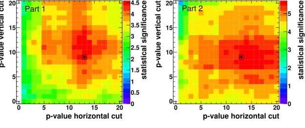
5.11 Statistical significance of the π

mass peak in the spectra of missing mass for the dd →

HeX reaction for different p-value cuts. . . 76

5.12 cos θ

of outgoing particle X in the c.m. coordinate system versus the missing mass for dd →

HeX. . . 77

5.13 Missing mass for the dd →

HeX reaction for −0.9 ≤ cos θ

≤ 0.4. . . 77

5.14 Missing mass for the dd →

HeX reaction for every cos θ

bin for 1st

part of the beamtime. . . 78

5.15 Missing mass for the dd →

HeX reaction for every cos θ

bin for the 2nd part of the beamtime. . . 79 6.1 Kinematic variables cos

, cos

, M

, ϕ describing the dd →

Henπ

reaction. . . 83 6.2 Difference between the reference luminosity and the luminosity for dif-

ferent cuts on p-value form the kinematic fit and the value of χ

of the kinetic energy reconstruction. . . 84 7.1 Angular distribution for the 1st and the 2nd part of the beamtime ob-

tained with the 2-body phase space generator of the signal. . . 86 7.2 Missing mass for the dd →

HeX reaction the most backward angular

bin −0.9 ≤ cos θ

< −0.6 fitted with the modified Monte Carlo template with the low mass region included. . . 87 7.3 Differential cross section for different p-value cut variation. . . 88 7.4 Differential cross section used to fix the parameters in the new signal

generator. . . 89 7.5 Missing mass for the dd →

HeX reaction for every angular bin for all

data. . . 90 7.6 Missing mass for the dd →

HeX reaction for −0.9 ≤ cos θ

≤ 0.4 for all

data. . . 91 7.7 Comparison of the acceptance times cut efficiencies for the dd →

Heπ

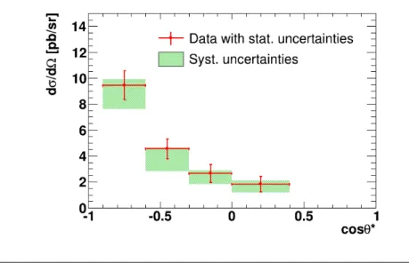
reaction for new and old generator as a function of cos θ

. . . 91 7.8 Differential cross sections for every angular bin. . . 93 7.9 Systematic uncertainties for the combined differential cross sections for

every angular bin. . . 94 7.10 Check of the systematic effects on the total cross section and the fit pa-

rameters of the angular distribution. . . 95 7.11 Final angular distribution. . . 96 8.1 Comparison between the angular distribution obtained in this thesis

and the previous WASA measurement of dd →

Heπ

. . . 98 8.2 World data on the unpolarised dd →

Heπ

total cross section. . . 99 8.3 Fit of the angular distribution with the fixed s-wave contribution from

the world data. . . 100 8.4 Correlation plot with the confidence regions for the parameters |C|

and

<{A

A

} . . . 101

List of Tables

3.1 Beam cycle structure. . . 32

3.2 Main properties of the beamtime. . . 34

4.1 Comparison of the fit parameters of M

for data and simulation. . . 61

5.1 Preselection conditions. . . 67

6.1 Results of the luminosity calculation for the 1st and the 2nd part of the beamtime. . . 82

7.1 Number of signal events in every angular bin. . . 90

7.2 Signal acceptance times cut efficiencies for every angular bin for the 1st

and the 2nd part of the beamtime. . . 91

List of Abbreviations

QCD Quantum Chromodynamics QED Quantum Electrodynamics SM Standard Model

χ

Chiral Perturbation Theory EFT Effective Field Theory CSB Charge Symmetry Breaking TRIUMF Tri-University Meson Facility WASA Wide Angle Shower Apparatus COSY COoler SYnchrotron

ToF Time-of-Flight FD Forward Detector CD Central Detector

FWC Forward Window Counter FPC Forward Proportional Chamber FVH Forward Veto Hodoscope MDC Mini Drift Chamber PSB Plastic Scintillator Barrel SCS Superconductive Solenoid

SEC Scintillator Electromagnetic Calorimeter DAQ Data Acquisition

FPGA Field-Programmable Gate Array

QDC Charge-to-Digital Converter

TDC Time-to-Digital Converter

FIFO First In First Out

Chapter 1

Introduction

Why does the Universe exist as it is?

For decades a multitude of physicists have been trying to understand and describe the structure of matter and basic interactions in Nature. Many mysteries of the existence of our Universe have been solved by curiosity-driven studies, but a lot of fundamental questions are still open.

Nowadays, we know that protons and neutrons, collectively called nucleons, form nuclei. Together with electrons, they build all the stable elements in the visible Uni- verse. Nucleons are not elementary particles, but they are built of quarks and gluons.

The basic constituents of protons and neutrons are the up (u) and down (d) quarks.

In the constituent quark model, the proton is made of two u and one d quark, while the neutron comprises of one d and two u quarks. In units of the elementary charge e, the charges of the u and d quarks are +2/3 and −1/3, respectively. Therefore, the proton has a positive charge 1e, and the neutron is neutral. However, in addition to the difference in charge, there is also a small difference in the u and d quark masses.

This tiny difference is vital for our very existence. In a world with equal masses of u and d quarks, the proton-neutron mass difference would be based exclusively on elec- tromagnetic effects. This would result in the proton being heavier than the neutron.

In such a world the proton, not the neutron, would have a finite lifetime, and stable hydrogen atoms would not exist. Our whole universe would not exist in the way it is now.

The importance of light quark mass effects has driven many theoretical and ex- perimental studies. The goal is to describe the effects induced by quark masses in hadronic reactions. It is to show that our understanding of the theory of strong inter- action — Quantum Chromodynamics (QCD), and especially the calculations based on it — is correct. The measurement of the dd →

Heπ

reaction provides an important experimental input to the calculations which trace the proton-neutron mass difference induced by the difference of u and d quark masses.

In this Chapter an introduction to the topic is given. Basic information about the

structure of matter, the origin of mass and the idea of isospin is discussed. A short de-

scription and the formalism of low energy hadron physics is described. In Chapter 2

the theoretical and experimental status of the selected charge symmetry breaking ob-

servables is presented. The experimental setup used in this measurement and the run

conditions are described in Chapter 3. The basic data analysis procedure, including the calibration of the detector and the tracking procedure as well as the Monte Carlo simulations, is reported in Chapter 4. The selection of the dd →

Heπ

reaction is described in Chapter 5. The luminosity determination is reported in Chapter 6. The results are presented in Chapter 7. A discussion of these results and an outlook in Chapter 8 complete the thesis.

1.1 Standard Model

1.1.1 Elementary Particles and Interactions

All the matter in the Universe is built of basic building blocks called elementary parti- cles, interacting with each other by four fundamental forces, namely the gravitational, electromagnetic, weak and strong force. Elementary particles and the interactions between them (with the exception of the gravitational force) are described within a quantum field theory called the Standard Model (SM). The schematic depiction of el- ementary particles included in the SM is presented in Fig. 1.1.

F

1.1: Elementary particles included in the Standard Model. The three generations of quarks and leptons are presented in the first three columns, gauge bosons are in the fourth column, and the Higgs boson

in the fifth one. Source: [1].

The elementary particles building all matter are fermions, which means they have a spin equal to

~. They are divided in two groups — leptons and quarks. Within each group there are three generations of pairs of particles. The first generation consists of the most stable and lightest particles, while the less stable and heavier ones belong to the higher generations.

Leptons are particles which do not interact via the strong force. For leptons, every

generation consists of one negatively charged particle, and one neutral partner, called

neutrino. Therefore, we have: electron and electron neutrino (e, ν

), muon and muon neutrino (µ, ν

), tauon and tauon neutrino (τ, ν

). Quarks interact strongly in addition to the other interactions. They are carriers of one of three colour charges. Quarks possess also an electric charge of +2/3 or −1/3 of the elementary charge e. The three families of quarks ordered by mass are: up and down quark (u, d), strange and charm quark (s, c), and bottom and top quark (b, t). In addition, every matter particle has an antiparticle with identical mass.

The Standard Model describes the interactions as the result of the exchange of force-carrier particles. These particles are the so-called gauge bosons and have a spin of ~. The weakest interaction described in the SM is the weak force. It is described as an exchange of W

, W

, and Z

bosons. They couple to quarks and leptons. Because of the large gauge bosons masses (M

= 80.4 GeV/c

, M

= 91.2 GeV/c

), the weak interaction has only a short range of about 10

m [2].

The exchange particles for the electromagnetic force are photons, which couple to all particles with an electromagnetic charge. Photons are massless, therefore this in- teraction has an infinite range. The theory of electromagnetic interactions — quantum electrodynamics (QED) — is unified with the theory of weak forces in the so-called Glashow-Weinberg-Salam model [3] (electroweak interactions).

The strongest of all four fundamental interactions is the strong force. It is carried by eight massless gluons which couple to quarks and to themselves. The range of the strong force is about the radius of a nucleon. In the theory of strong forces, Quan- tum Chromodynamics (QCD), there are three types of strong charges, called colour charges. A quark can carry one of three primary colours (red, blue and green), and its antiquark carries the corresponding anticolour. Gluons carry one colour and one anti- colour. All composite particles made of quarks, called hadrons, have zero net colour, i.e., they are colour singlets. Particles built of quark and anti-quark are called mesons, while particles consisting of three quarks are called baryons [4].

1.1.2 Color Confinement

The Standard Model is a quantum field theory based on the gauge invariance of the group SU (3)

× SU (2) × U (1). Quantum Chromodynamics is the SU (3)

component of the Standard Model symmetry group. The remaining SU (2) ×U (1) is the symmetry group of the electroweak theory. For an introduction to quantum field theory see, e.g., [5, 6].

Most calculations in Quantum Field Theory are performed in an approximated

way using perturbative methods based on an expansion in powers of the coupling

constant. This method is applicable only in the limit of a small coupling constant

α 1. The coupling constant determines the strength of the force exerted in an in-

teraction. The effective coupling constant varies with the energy scale. For QED it

grows with energy. At large distances, i.e, low four-momentum transfer Q

, it is about

α ≈ 1/137, at the scale of the Z boson it is about α ≈ 1/128 [2]. At very high ener-

gies, where the Standard Model is no longer applicable, the coupling becomes large

and eventually diverges. In QCD the self-coupling of gluons affects significantly this so-called running of the coupling constant α

. The strong coupling becomes weak for processes involving large four-momentum transfers. This phenomenon is called asymptotic freedom. At the scale of the Z boson α

is about 0.12 [2]. At small four- momentum transfers α

diverges.

One can introduce a QCD energy scale Λ

— the energy scale at which the perturbatively-defined coupling constant α

would diverge. The effective strong cou- pling constant can be presented then as:

α

(Q

) = 2π

β

log(Q

/Λ

) , (1.1) where β

= 11 − 2/3n

, and n

is the number of quark flavours. The value of Λ

can be determined experimentally by measuring the dependence of α

on the four- momentum transfer Q

. The obtained value is about Λ

≈ 250 MeV [7].

For the perturbative region, Q

Λ

, the quark and gluon degrees of free- dom dominate. At low four-momentum transfer, below Λ

, quarks and gluons are strongly confined. They cannot be observed as a free particles, but they form colour neutral objects, called hadrons. The theoretical description of strong interaction in this region, referred to as "strong QCD", relies on lattice gauge theory, phenomenological models or effective field theories.

The strong coupling constant α

is one of the parameters of QCD. Like α, it has to be extracted from measured observables by theoretical calculations [3]. The general properties of the QCD and QED coupling constant are presented in Fig. 1.2.

F

1.2: Schematic behaviour of the coupling constants of QCD and QED. In QED, for low four-momentum transfers Q

the coupling con- stant is small. It increases as a function of Q

and at very high energy it diverges. For QCD the coupling at small Q

diverges and for high Q

it asymptotically goes to zero. Note that this picture shows only the general behaviour for the coupling constant of QCD and QED and the

scale on the x-axis is different for these two curves. Source: [8].

1.2 Origin of Mass

The Standard Model includes one additional particle - the recently discovered Higgs boson [9, 10]. The discovery confirmed the theory of the Brout-Englert-Higgs mech- anism [11–15]. This mechanism explains the generation of the intrinsic mass of the gauge W and Z bosons. Elementary particles can couple to the quantum excitation of the Higgs field (Higgs boson) and this endows them with an effective mass. The par- ticles coupled to this field are quarks, leptons, W and Z bosons, and the Higgs boson by itself.

The ordinary matter in the Universe is built of protons, neutrons and electrons, and protons and neutrons are made of quarks and gluons. However, only a few percent of the nucleon mass is coming from the intrinsic masses of the quarks themselves [16].

For example, for the proton (M

= 938 MeV/c

) the intrinsic masses of u and d quarks would contribute only about 10 MeV/c

to its mass. All the rest has its origin in the dynamics of the strong processes inside the nucleon [17, 18].

In the limit of massless quarks, the global chiral symmetry (SU (n)

× SU (n)

= SU (n)

× SU (n)

, where n is the number of quark flavours) of the QCD Langrangian is not broken explicitly. It is broken spontaneously through the formation of a quark condensate in the ground state to the isospin symmetry group SU (n)

. This quark condensate is a fermionic condensate formed by quark-antiquark pairs [19]. Quarks interact with this environment as though they had mass. One can imagine it as mass- less quarks traveling at the speed of light which are slowed down by the interaction with the quark condensate. Thus, they can be described as massive quarks in a free environment [17]. The nonperturbative scale of the dynamical chiral symmetry break- ing Λ

is about 1 GeV [2, 20]. Because of the small non-zero quark masses, the chiral symmetry is also broken explicitly. For quarks with masses M > Λ

the explicit chiral symmetry breaking dominates (c, b and t, the so-called "heavy" quarks). For M < Λ

the spontaneous chiral symmetry breaking is dominating (u, d and s).

As a result of the spontaneous chiral symmetry breaking for vanishing quark masses, according to the Goldstone theorem [21], massless Nambu-Goldstone bosons should be observed. Their number is determined by the structure of the symmetry group. For the SU (2)

× SU (2)

→ SU (2)

symmetry (u, d quarks considered) there are three Nambu-Goldstone bosons, one for each of the three generators of the sponta- neously broken symmetry, corresponding to the three pions (π

, π

, π

). The sponta- neously broken SU (3)

× SU (3)

symmetry (u, d and s quarks considered) has eight generators, therefore there are eight Nambu-Goldstone bosons (π

, π

, π

, η

, K

, K ¯

, K

, K

). Because of the explicit chiral symmetry breaking caused by non-zero quark masses, the Nambu-Goldstone bosons have also small finite masses [22].

The main origin of the ordinary mass is thus not the Higgs mechanism, but rather

is a consequence of the spontaneous breaking of chiral symmetry. For a popular intro-

duction to the topic see [16, 23]. Detailed information about the origin of mass can be

found in [17].

1.3 Chiral Perturbation Theory

An analytic derivation of hadronic interactions from the fundamental QCD La- grangian is still not achieved. However, what is known are the symmetry features of the strong interaction. The chiral symmetry properties of QCD are the key compo- nents of Chiral Perturbation Theory (χ

) [24, 25], which is an effective field theory (EFT) for low energy QCD.

The concept of an EFT can be presented as a theorem [25, 26] which states that, if the calculations are based on the most general interaction consistent with the symme- tries and symmetry-breaking patterns of the underlying fundamental theory (in our case QCD), the results will be consistent with those of the underlying theory up to a given order in perturbation theory. In χ

the dynamic degrees of freedom [27] are not the fundamental quarks and gluons but the lightest pseudoscalar mesons identi- fied as the Nambu-Goldstone bosons of the spontaneously broken chiral symmetry, which are non-interacting in the chiral limit for vanishing momenta.

As χ

is built for low energy QCD, it takes explicitly into account the relevant degrees of freedom, which are the states with M Λ

, where Λ

is a hadronic scale already mentioned in Sec. 1.2. Heavier excitations are integrated out from the action.

Only because the pseudoscalar octet is separated on the mass scale from the rest of the hadronic spectrum, it is possible to construct this EFT.

The fields of the Nambu-Goldstone bosons are represented in the chiral La- grangian by the unitary matrix U = exp(i √

2Φ/f ), where the most common form of Φ is:

Φ =









√1

2

π

+

6

η

π

K

π

−

2

π

+

η

K

K

K ¯

−

2

η









, (1.2)

and f is the Nambu-Goldstone boson decay constant in the chiral limit.

At low energies, the interaction between Nambu-Goldstone bosons can be ex- panded in powers of their momenta p, which are small compared to Λ

. Powers of momenta correspond to powers of derivatives of the Nambu-Goldstone boson fields in the χ

Lagrangian. The explicit chiral symmetry breaking is introduced in the χ

Lagrangian via the quark mass matrix M . Therefore, in addition to the derivative ex- pansion, the effective Lagrangian is expanded simultaneously in powers of M , which is possible since the quark masses are much smaller then Λ

. Below, the lowest order effective chiral Lagrangian L

is presented. It shares the same symmetry patterns with QCD: C, P, T, Lorentz invariance and, in particular, chiral symmetry. The first term in L

represents the effective χ

Lagrangian for the limit of massless quarks.

The second term introduces the explicit chiral symmetry breaking [28].

L

= f

4 h∂

U

∂

Ui + f

B

2 hU

M + M

U i, (1.3)

where M is the quark mass matrix for p = 0. The constants B and f are not fixed

by symmetry requirements alone. The physical meaning of the chiral coupling f at the considered order is, that — in the chiral limit — it is the pion decay constant (f

≈ 92.4 MeV). Also in the chiral limit, B is directly related to the chiral condensate:

h0|¯ qq|0i = −Bf

+ O(M

). Thus, B is the order parameter of spontaneous chiral symmetry breaking. The value of B ≈ 1800 MeV has been extracted from the sum- rule value h0|¯ qq|0i = −(250 MeV)

[29].

An effective field theory can be also introduced for mesonic resonances and baryons [30, 31]. However, the fact that in the chiral limit baryon masses do not vanish and that they are not small compared to Λχ complicates the chiral analysis of baryons [27]. χ

has been successfully extended to pion production where typical momenta are in the order of √

m

M , where M is the nucleon mass (for a review see [32]). A com- plete description of the interactions in the baryonic sector based on χ

requires to fix the strength of the hadronic operators either from experiment or from lattice QCD cal- culations. For the πN interaction, at leading order the only parameters are the pion mass and pion decay constant [33, 34], but for higher orders the number of unknown parameters increases. The theory, however, can provide non-trivial links between the different operators, which need to be fixed by experiment. Therefore, an investigation of the basic symmetries of the strong interaction requires an joint effort of experiment and theory.

1.4 Isospin

1.4.1 Isospin Multiplets

After the discovery of the neutron in 1932 by Chadwick [35], the similarity between the proton p and the neutron n led to the idea of the existence of an approximate symmetry. It was suggested that both may be treated as two states of the same par- ticle, namely the nucleon N . This requires that neutron and proton have the same mass. In fact, their masses are only approximately equal (m

= 939.57 MeV/c

, m

= 938.28 MeV/c

[2]). It was suggested that nucleons behave identically under the strong interaction and that the only difference between these two states has its origin in their charge content: isospin symmetry would be a good symmetry of the strong interaction. A strong isospin quantum number was introduced, with the projection coordinate T

equal to +1/2 for protons and −1/2 for neutrons.

The symmetry group of the rotation operators in isospin space is a SU (2)

group with operators represented as:

U ˆ

(α) = ˆ U

(α

, α

, α

) = e

= e

. (1.4) The angles α = {α

, α

, α

} describe the rotations around three axes in the abstract isospin space, and τ

are the Pauli matrices.

The isospin multiplets can be introduced in the same way as the angular momen-

tum and spin multiplets. Each multiplet is (2T + 1) times degenerate. The nucleon

isospin doublet |T, T

i consists of proton and neutron states with T =

:

1 2 , 1

2

≡ |pi ,

1 2 , − 1

2

≡ |ni .

(1.5)

The isospin triplet with T = 1 is realized in nature, e.g., for π mesons:

|1, 1i ≡ π

,

|1, 0i ≡ π

,

|1, −1i ≡ π

.

(1.6)

Let us now consider the isospin of the deuteron. Each deuteron consists of one proton and one neutron and its wave function can be described in terms of the con- stituent nucleons. Therefore, the third component of its isospin T

equals to 0. The first possibility is that the deuteron is an isospin singlet state |0, 0i :

|0, 0i = 1

√

2 (|pi |ni − |ni |pi) . (1.7) Another option is that the deuteron is the isospin state |1, 0i from the triplet:

|1, 1i = |pi |pi ,

|1, 0i = 1

√ 2 (|pi |ni + |ni |pi) ,

|1, −1i = |ni |ni .

(1.8)

Because of isospin symmetry, all triplet states should have comparable energy. Thus, if the deuteron was an isotriplet |1, 0i , nn and pp bound states should have been ob- served in nature. This is not the case. Therefore, the deuteron has to be the isospin sin- glet state |0, 0i . With similar arguments one can show that the nucleus of

He (which is build of two protons and two neutrons) is also an isosinglet state.

Within the Standard Model, the isospin symmetry of the proton and the neutron can be reinterpreted as the isospin symmetry of the u and d quarks. Then the funda- mental isospin doublet of the up and down quark states is:

|ui ≡ 1 2 , 1

2

,

|di ≡ 1 2 , − 1

2

.

(1.9)

In the framework of the constituent quark model the proton and the neutron can be

represented as totally symmetric uud and udd states. The pion triplet can be presented

as:

π

≡ u d ¯

,

|π

i ≡ 1

√

2 |u¯ ui − d d ¯

, π

≡ |d¯ ui .

(1.10)

1.4.2 Isospin Symmetry Violation

In the Standard Model there are two sources of isospin symmetry violation. The first natural source is the charge difference of the different quarks. The charges of the lightest quarks are Q

= 2/3e and Q

= −1/3e (convention: e > 0). In addition, isospin symmetry is broken by the strong interaction because the quarks also have slightly different masses [36, 37]. In order to study the effects caused by the quark mass difference, these two sources of isospin symmetry breaking need to be disentangled.

The isospin symmetry breaking on the hadronic level manifests itself in several static observables. One observable, which is important for our very existence, is the proton-neutron mass difference ∆M

. As the quark mass difference, it has two ori- gins: an electromagnetic and a strong one. If isospin symmetry was broken only be- cause of the different charges of the lightest quarks, ∆M

would be a purely electro- magnetic effect, with the result that the proton would be heavier then the neutron, and that stable hydrogen atoms would not exist. However, nature shows that this is not the case and that the proton as a stable particle (with a mean lifetime τ

> 10

yr) is lighter then the neutron (τ

≈ 880 s). Thus, ∆M

has an additional contribution from the strong interaction:

∆M

= ∆M

+ ∆M

. (1.11)

The electromagnetic part ∆M

can be calculated based on QED considerations and dispersion theory [38], where ∆M

can be obtained indirectly (∆M

=

∆M

− ∆M

) [37, 39], from lattice QCD [40], or from χ

calculations. Chiral per- turbation theory provides an interesting link between the static isospin breaking ob- servable ∆M

and, at leading order, the dynamic isospin violating πN scattering length [36].

In general, experimentally it is difficult to get access to quark mass effects in low energy hadron physics, where the effect of the pion mass difference ∆π = M

− M

, which is of electromagnetic origin, is by far dominant [41]. Therefore, any observables where ∆π does not contribute are of interest. Here, charge symmetry breaking (CSB) play a major role.

1.4.3 Charge Symmetry Violation

Charge symmetry is a special case of isospin symmetry. It is the invariance under the

rotation of an angle of 180

in isospin space around the T

axis. The charge symmetry

operator is:

U ˆ

= e

. (1.12)

The pion mass difference ∆π is invariant under this rotation and does not contribute to charge symmetry observables. U ˆ

transforms the π

state into a π

, and m

= m

because of CPT symmetry. Simply speaking, charge symmetry is the symmetry under interchange of the u and d quarks [42]:

U ˆ

|ui = − |di ,

U ˆ

|di = |ui . (1.13)

Charge symmetry breaking (CSB) manifests itself in many phenomena like the differ- ent scattering lengths in nn and pp systems after correcting for electromagnetic effects [43], neutron–proton elastic scattering at intermediate energies [44], π − η mixing [45, 46], or the Nolen–Schiffer anomaly in the binding energy difference of

H and

He [47, 48]. In 1977 Weinberg predicted an effect of CSB in πN scattering [36]: the differ- ence in the scattering lengths for nπ

and pπ

should be huge (up to 30%) and directly proportional to M

. However, the direct measurement of f (π

p) − f (π

n) in πN scattering is practically impossible experimentally, because of the lack of π

beams.

Thus, there was the suggestion [49, 50] to use N N induced pion production as an alternative access to CSB pion–nucleon scattering. There have been three successful experiments in which the corresponding CSB observables were measured:

• the forward-backward asymmetry A

in the np → dπ

reaction [51],

• the total cross section of the reaction dd →

Heπ

near the threshold [52],

• the total and differential cross section of the reaction dd →

Heπ

at an excess energy of Q = 60 MeV [53].

The study presented in the thesis concentrates on a new measurement of the dd →

4

Heπ

reaction. In the next chapter the theoretical and experimental status of the CSB

reactions presented above is discussed.

Chapter 2

Experimental and Theoretical Status

In this chapter a description of the experimental and theoretical status of three CSB observables — the forward-backward asymmetry A

in the np → dπ

reaction and the total and differential cross section of the reaction dd →

Heπ

near the threshold

— is presented. These observables provide an alternative access to CSB effects of the pion–nucleon scattering.

2.1 Forward-Backward Asymmetry in np → dπ ⁰

The forward-backward asymmetry A

of the np → dπ

reaction was measured at Canada’s National Laboratory for Particle and Nuclear Physics TRIUMF. A neutron beam with an energy of 279.5 MeV was impinged on a proton target, corresponding to an excess energy, ε, of about 2 MeV [51]. A

is defined as:

A

= R

0

h

dΩ

(θ) −

(θ − π) i

sin θdθ R

0

h

dΩ

(θ) +

(θ − π) i

sin θdθ

, (2.1)

where θ is the emission angle of the deuteron in the center of mass frame. In Fig. 2.1 the scheme of the np → dπ

reaction in the c.m. system before and after an interchange of u and d quarks is presented. The angle between the proton and deuteron before the interchange is equal to θ, and afterwards it is equal to π − θ. Therefore, if the charge symmetry is broken, the differential cross section is not symmetric and A

6= 0. The experimentally obtained value is A

= [17.2 ± 8(stat.) ± 5.5(syst.)] · 10

[51]. The result has a quite big uncertainty: within two standard deviations of the statistical uncertainty it is compatible with zero.

The first theoretical calculations of A

based on a meson-exchange coupled-

channel formalism are presented in [54]. It was predicted that π − η mixing should

completely dominate this observable. The calculated asymmetry A

= −28 · 10

is negative, contrary to the experimental result. First calculations based on χ

[49],

where the CSB effects were modeled by a charge symmetry violating π

N interaction,

lead to a value of A

= 60 · 10

which is much larger than the one observed exper-

imentally. Both calculations were performed before the results appeared describing

mechanisms of isospin conserving pion production in the NN − − → NNπ reactions in

χ

[55, 56]. These developments provided a good base for studying isospin violation

F

2.1: Scheme of np → dπ

reaction in the c.m. system, before (left) and after (right) an interchange of u and d quarks.

effects and brought the total cross section and the angular distribution into agreement with the experiment [50, 57]. It has been shown that at leading order (LO) A

is di- rectly proportional to M

, while the effect of π − η mixing is subleading. The leading order diagram for the CSB s-wave amplitudes of the np → dπ

reaction is depicted in Fig. 2.2. From the experimental value of A

, M

was obtained as

∆M

= 1.5 ± 0.8(exp.) ± 0.5(th.) MeV . (2.2) This value is in agreement with lattice predictions [40] and the indirect extraction from

∆M

= ∆M

− ∆M

[37, 39].

F

2.2: Leading order diagram for the CSB s -wave amplitudes of the np → dπ

reaction. The solid lines represent nucleons, the dashed lines denote pions, the cross indicates the CSB vertex and the dot rep-

resents a leading order charge invariant vertex. Source [50].

2.2 Total and Differential Cross Section of dd → ⁴ He π ⁰

2.2.1 dd →

Heπ

Cross Section Close to Threshold

The total cross section of the dd →

Heπ

reaction was first measured at the In-

diana University Cyclotron Facility at two different beam energies. The results are

σ = 12.7 ± 2.2 pb and σ = 15.1 ± 3.1 pb at 228.5 MeV and 231.8 MeV beam energy

[52], respectively. In Fig. 2.3 the

He missing mass for dd →

HeX is presented. Each

spectrum shows a prominent signal on top of a continuous background. The spectra

are described by a Gaussian peak and a continuum, presented as curves. The energy dependence of these results are comparable with s-wave pion production.

F

2.3: Candidate events at the two deuteron bombarding ener- gies 228.5 MeV and 231.8 MeV as a function of the

He missing mass for dd →

He X . The smooth curves show the reproduction of these

histograms with Gaussian peak and a continuum. Source [52].

2.2.2 Theory

When the charge symmetry operator acts on the particular hadronic states from the dd →

Heπ

reaction, one gets:

U ˆ

|di = |di , U ˆ

He

=

He

, U ˆ

π

= − π

. (2.3)

The dd →

Heπ

reaction violates charge symmetry because the system

Heπ

, odd under charge symmetry, should not be produced from the dd system, which is even under charge symmetry. Therefore, the total cross section is proportional to the CSB amplitude |M

|

.

First calculations for the dd →

Heπ

reaction can be found in [58, 59]. In [58] a simplified set of d and

He wave functions and a plane-wave approximation for the initial dd state were used. The ordering scheme of χ

was used to classify and iden- tify different contributions. At leading order, there is only the contribution from πN re-scattering; no next-to-leading order contribution is identified. It occurred that the formally leading πN re-scattering term is suppressed due to selection rules in spin and isospin space. The contributions from next-to-next-to-leading order (NNLO) di- agrams were too small to account for the observed cross section. It was shown that better agreement could only be obtained if short-range pion emission was taken into account.

More reliable calculations were performed in [59], where realistic two- and three-

nucleon interactions in a χ

calculation were used. This allowed a proper treatment

of the effects of the deuteron-deuteron interaction in the initial state and to use a re-

alistic

He bound-state wave function. The contribution of the leading order term

for the s-wave channel is confirmed to be suppressed. The contributions at NNLO individually give results of the same order as the experimental cross section. This demonstrates the significant influence of the initial-state interaction. A complete cal- culation to NNLO — including pion loops and CSB in the initial state — is still under investigation.

The effects of initial-state Coulomb interactions were investigated in [60] using a simplified set of d and

He wave functions and a plane-wave approximation for the initial dd state. It was shown that the cross sections for dd →

Heπ

can be significantly enhanced by the soft photon exchange.

Furthermore, [61] shows that using parameters consistent with the CSB induced difference between the strong pp and nn scattering one can provide significant con- straints on the calculated amplitude for the dd →

Heπ

reaction. However, the result is very sensitive to the choice of the nuclear potential model, which demonstrates that a simultaneous analysis of the N N scattering length and the dd →

Heπ

reaction is needed.

There is one more important test for the theoretical description of the CSB ob- servables. At NNLO the first counter term enters the s-wave pion production with unknown strength D. In addition, the isospin violating ¯ πN N coupling constant β

contributes. The reaction dd →

Heπ

near threshold can be used together with the forward-backward asymmetry in np → dπ

to NNLO to fix D ¯ and β

(the required evaluation of the transition operator to one loop is in progress). Once the parameters are fixed, the p-wave contribution can be predicted parameter-free to leading and next- to-leading order, which will provide an important cross-check for the χ

predictions [62].

In Fig. 2.4 some formally leading operators for p-wave pion production are pre- sented. The coupling strengths are given by the leading CSB πN amplitude (Fig. 2.4 a) and the leading CSB πN N vertex (Fig. 2.4 b and 2.4 c). However, as for the s-wave pion production, the contribution of diagram (a) is suppressed as a consequence of selection rules. Therefore, p-wave pion production provides direct access to the CSB πN N coupling constant β

. A measurement of the p-wave contribution in dd →

Heπ

is therefore complementary to the np → dπ

measurement from [51] which is mostly sensitive to the leading isospin violating πN amplitude [62].

In addition, higher partial waves are predicted to be sensitive to the CSB NN − − → N∆ transition potential which is difficult to access in other reactions. This potential is known in chiral perturbation theory in LO. Therefore, the measurement of higher partial waves provides an additional non-trivial test of the understanding of isospin violation in hadronic reactions [53].

2.2.3 Charge Symmetry Breaking with WASA-at-COSY

The investigation of higher partial waves of the pion production in the dd →

Heπ

reaction at ε = 60 MeV is one of the main goals of the WASA-at-COSY experiment.

The program started with the measurement of the isospin conserving dd →

Henπ