Minicharged Particles from the Sun:

Prepared for submission to JCAP

MPP-2015-199

Minicharged Particles from the Sun:

A Cutting-Edge Bound

N. Vinyoles,

H. Vogel

a

Institute of Space Sciences (CSIC-IEEC),

Campus UAB, Carrer de Can Magrans, S/N, 08193 Cerdanyola del Vall` es, Spain

b

Max Planck Institute for Physics (Werner Heisenberg Institute), F¨ ohringer Ring 6, D-80805 M¨ unchen, Germany

E-mail:

Abstract. We study the impact on the Sun of an exotic energy-loss channel caused by

plasmon decay into fermionic minicharged particles with charge e and mass m

. We

compare solar models with this extra emission to helioseismological and neutrino data,

obtaining a bound < 2.2

10

(95% CL) for m

25 eV. Our result is comparable

to previous limits from the cooling of globular cluster stars, while at the same time it is

better understood and takes theoretical and observational errors into account.

Contents

1 Introduction 1

2 The Sun 4

2.1 Observables

2.2 Standard Solar Models

3 Minicharged particles 5

3.1 Models without a hidden photon

3.2 Models with a hidden photon

3.3 Production and propagation of minicharged particles

3.3.1 Production

3.3.2 Propagation

3.4 Analytical estimate

4 Statistical method 9

5 Minicharged particles in the Sun 10

5.1 Sound speed profiles

5.2 Neutrino fluxes

6 Results 14

7 Discussion and summary 16

A Collider constraints on minicharged particles 18

B Neutrino magnetic moments 18

1 Introduction

Our Sun is a powerful laboratory. Its large density, temperature and shear size allow us to study physics in environments that are hard to reproduce in earth-based experiments.

Its proximity, on the other hand, allows us to measure and understand the Sun in great detail. Major breakthroughs have been achieved in the past by observing, e.g., neutrinos from proton–proton fusion [1] or neutrino flavor oscillations [2].

The Sun is the most studied star and information from observations and theoretical

models are available to look into its inside. Helioseismology [3], the study of the global

oscillations of the Sun, allows us to extract information on the Sun’s structure, e.g., the

sound speed profile, the convective radius and the surface helium abundance. Moreover,

the measurement of the solar neutrino fluxes enables us to extract information on the solar

interior through an independent channel. These observations combined with the accurate

Standard Solar Models (SSMs) [4,

evolution. Although some inconsistency remains [6,

broadly agree.

This agreement allows us to constrain any contribution that might arise from non- standard physics. Weakly-interacting, low-mass particles like the axion [8] and axion-like particles (ALPs), hidden photons [9–11], or minicharged particles (MCPs), e.g. [10,

can be produced copiously inside the Sun. If the couplings of the exotic particles are so large that they are trapped, they contribute to the Sun’s energy transport, potentially changing its composition and evolution drastically. For smaller couplings, they carry energy out of the Sun which changes the solar evolutionary structure. By comparing this structure with observations, one can derive stringent bounds on extra energy sinks. This energy-loss argument has been applied a number of times to the cooling of WDs [13–17]

and supernovae (SNe) [18,

of horizontal branch (HB) stars [14,

the Sun [21,

extreme objects since it is less dense and hot. However, we will show that this detriment is compensated by the quality and amount of data available.

In this work, we focus on the energy-loss argument for minicharged particles produced in the Sun. Although the charge of all observed particles seems to be quantized and a multiple of the down-quark’s charge, there is no a priori theoretical reason for charge quantization in the particle Standard Model (SM). This mystery has led to a continuous effort of experimental searches [31,

quantization allows theorists to postulate the existence of a particle that couples to the SM photon with an arbitrary charge, the MCP. Such a particle can either be studied as an ad hoc extension of the SM, or it might be predicted by more intricate models, for example theories with an additional unbroken U (1)

gauge symmetry [10,

sectors (e.g. [43,

e, where is the minicharge parameter (’minicharge’) and e is the charge of the electron. The size of the minicharge depends on the model assumptions and can be very small (e.g. [45–50]).

We will in the following consider as a free parameter.

Minicharged particles couple to the electromagnetic plasma inside the Sun, which con- tains a thermal bath of collective excitation modes (’plasmons’). These plasmons can de- excite, thereby emitting a pair of MCPs. The rate of this decay depends on the minicharge but also on the plasma frequency ω

of the Sun and the MCP mass m

since the decay into MCPs becomes kinematically disfavored for large MCP masses, 2m

> ω

. Once produced, the small minicharges we consider here allow the MCPs to escape the Sun unimpeded, giving rise to an additional energy-loss channel.

To limit this emission from the Sun, we use the statistical method described in ref. [26]

that combines most of the available information on the Sun: observational (neutrino fluxes and helioseismology) and theoretical (SSMs) data taking into account the corresponding errors and correlations. This leads to a conservative bound (95% CL) of

< 2.2

10

for m

< 25 eV , (1.1) on the minicharge for low-mass MCPs, which is comparable to the limits < 2

10

obtained by red giants and horizontal branch stars [14]. Equivalently, we find that an emission of up to 1.5% of the Sun’s total luminosity can still be viable for these MCPs.

The exact mass dependence of our bound can be seen in fig.

together with a summary of limits that have been obtained previously from various experiments and observations

.

1Figure1also includes updated limits from dark radiation [29] and colliders [31,32].

2 4 6 8 10 12 14 -14

-12 -10 -8 -6 -4 -2 0

Log10(mf/eV) Log10(ϵ)

RG WD HB

OPOS

COLL

SLAC

BBN Yp

CMB Neff

SN 1987A

CMB DM LHC

TEX

E613

Sun

XENON10

2 4 6 8 10 12 14

-14 -12 -10 -8 -6 -4 -2 0

Log10(m_f/eV) Log10(ϵ)

RG WD HB

OPOS

COLL

SLAC

B B N SN 1987A

LHC TEX

E613

Sun

XENON10

DM CMB

Figure 1. Summary of constraints on fermionic MCPs in the mass/minicharge plane. The result of this work is depicted in yellow. Left panel: Models with a massless hidden photon for aU(1)h

gauge coupling g⁰= 0.1 (see sec. 3). We updated the CMB and BBN bounds from ref. [29] using 2015 Planck data [30], and the collider bounds (COLL) from refs. [31,32]. The remaining bounds are from DM [31], CMB [33], LHC [34], SLAC [35], OPOS [36], TEX [37], E613 [38], and HB, WD, RG [14, 29]. The Xenon10 bound is plotted with dashed lines since it is an estimate taken from a higgsed model of minicharged particles [39]. Right panel: Bounds on models without a hidden photon. The dark radiation bounds from ref. [29] disappear but the limits from overproduction [31]

and distortions of the CMB [33] become far more constraining.

The plots show the two most popular scenarios that involve MCPs. The bottom-up approach minimally adds an additional particle with arbitrary charge, the MCP, to the Standard Model. This is plotted in the right panel of fig.

scenarios generate a minicharge through the kinetic mixing of the SM photon with a new massless photon. Some bounds on MCPs rely on this new ’hidden’ photon, so that the summary plot changes drastically for large MCP masses. The bounds for this model are shown in the left panel of fig.

yellow. As apparent from the figure, the bound of this work is among the most constraining for low-mass MCPs.

Our result is especially interesting because the bound is more robust than previous limits and contains statistical information that is absent for bounds obtained from RGs and HB stars. Additionally, our Sun is not only better observed than any other astrophysical object, future improvement of our understanding is to be expected as well. Additional insight can be achieved by the new generation of neutrino experiments, the possibility of observing g-modes [51], which will give direct information on the center of the Sun, or new opacity experiments (e.g. [52]) among other improvements. This will very likely make the Sun the most constraining source for low-mass MCPs in the foreseeable future.

The plan of the paper is as follows. We present the observational and theoretical

status of the Sun in sec.

comments on their propagation can be found in sec.

by the

statistical method applied in this paper. We then introduce the MCP into the SSMs in

AGSS09 Observables Ref.

Y

0.232(1

0.013) 0.2485

0.0035 [55],[6]

R

/R

0.7238(1

0.0033) 0.713

0.001 [55],[6]

Φ(

Be) 4.56(1

0.06) 4.82(1

) [56], [57]

Φ(

B) 4.60(1

0.11) 5.00(1

0.03) [56],[57]

Table 1. Theoretical and observational values for the surface helium Ys, the convective radius RCZ, the neutrino flux from⁷Be and from ⁸B. The second column shows the SSM values for the AGSS09 composition with the corresponding model errors [53]. The third column summarizes the observational and experimental values and errors. Neutrino fluxes are in 10⁹cm⁻²s⁻¹ for Φ(⁷Be) and 10⁶cm⁻²s⁻¹ for Φ(⁸B).

sec.

and comment on changes of the observables. The values of our resulting bounds on are presented in sec.

2 The Sun

The key advantage in using the Sun lies in the amount of available information. Our goal is to combine the helioseismology data and the neutrino solar observations (see sec.

with solar models (see sec.

minicharged particles. In this section, we describe the available information on the Sun that we use for this purpose.

2.1 Observables

The most important information on the Sun comes from helioseismology and from the detected neutrino fluxes. Helioseismology allows us to determine the sound speed profile.

This can be done by inverting the observed frequencies of solar oscillations, providing a direct test of the structure of the solar interior. From helioseismology, we can also derive the surface helium abundance and the radius of the convective zone [3]. In particular, we use as observables 30 points of the sound speed profile with radii r < 0.8R

from ref. [54], the surface helium Y

and the convective radius R

. From the neutrino observations, we consider the neutrino fluxes from

B and

Be. We do not use the pp and pep neu- trino fluxes because the experimental errors are still too large to be statistically relevant.

The observational values and the corresponding errors of the surface helium, radius of the convective zone and the neutrino fluxes are the same values as used in ref. [26] and are summarized in tab.

together with the values of the AGSS09 solar model and the corresponding theoretical errors.

2.2 Standard Solar Models

Standard Solar Models are theoretical descriptions of the Sun that are calibrated to match

the Sun’s present status. They are calculated by adjusting three initial quantities (initial

helium, mixing length and initial metallicity) to satisfy the present solar luminosity L

=

3.8418

10

erg s

, the solar radius R

= 6.9598

10

cm and the metal-hydrogen

ratio (Z/X )

. This last ratio will determine the composition and distribution of metals in

the interior of the Sun. Nowadays, the solar value of this ratio is still under debate. The

main discussion is among two different compositions: The old compilation of abundances,

GS98 [58], gives a value of Z/X

= 0.0229 and a resulting thermal stratification close to observation. On the other hand, the new composition AGSS09 [59] has been extracted using a more accurate analysis with 3D hydrodynamical models of the solar atmosphere and an improved solar spectroscopic analysis giving a metal-hydrogen ratio (Z/X)

= 0.0178. However, the resulting thermal stratification is worse compared to observations than for the older composition. This is the so-called

One reason for this discrepancy could be that the radiative opacities, that together with the composition define the thermal stratification of the Sun, should be revised [53,

recent calculation of the iron opacity [52] gives a larger value than the one predicted for solar temperatures, which goes in the direction of relieving the solar abundance problem.

For more details about the compositions and the solar abundance problem, we refer the reader to refs. [6,

In this work, we use GARSTEC (GARching STEllar Code) [61] to calculate the SSMs.

Details on the parameters used can be found in section 2.1 of ref. [26]. In order to accommodate MCPs, the code has to be modified to account for the extra energy carried away. This energy-loss from MCPs will be explained in the next section.

3 Minicharged particles

The Standard Model of particle physics can be extended by consistently introducing new fields. In this work, we derive a bound for the minimal extension of just adding a minicharged field to the SM Lagrangian. However, our bounds are also applicable to more extended models like MCPs accompanied by a massless hidden photon and more intricate hidden sectors with very massive degrees of freedom.

3.1 Models without a hidden photon

The Standard Model gauge groups do not prevent us from adding charged, massive par- ticles to our theory. Indeed, a SU (2)

singlet, the MCP, can always be added to the SM Lagrangian

,

L

=

+ ¯ f (i / ∂

m

)f + eA

f γ ¯

f , (3.1) where f denotes the minicharged fermion with a mass m

(the MCP), is the minicharge parameter (’minicharge’) and A

is the SM photon’s vector potential. The minicharge is given by the charge quantum number of the MCP, which can be arbitrary small. This charge leads to a coupling between the MCP and photons, which also allows plasmons inside the Sun to decay into MCPs.

3.2 Models with a hidden photon

Minicharged particles can be naturally obtained when a local, unbroken gauge group U (1)

is added to the SM groups [10,

h denotes ’hidden’ meaning that SM particles will not be charged under the U (1)

. The Lagrangian for this model reads

L

=

+ ¯ f (i / D

m

)f

1

4 F

F

κ

2 F

F

, (3.2)

where the U (1)

manifests itself in a field strength tensor F

with a vector potential A

,

which describes the hidden photon. Again, ’hidden’ means that no SM particle couples

to the hidden photon. In contrast, F

is the field strength tensor of the SM photon.

Both photons have identical quantum numbers such that they can mix kinetically with an approximate mixing angle κ [last term of eq. (3.2)]. Such a mixing should not be omitted in generic models, and can also arise from loops of heavy particles charged under both, hypercharge and the hidden U (1)

[42]. The covariant derivative is

D

= ∂

ig

A

, (3.3)

where g

is the U (1)

gauge coupling of the fermion f . We also assume that f does not interact through other channels than the hidden photon.

The fermion f manifestly becomes a MCP when the equations of motion of the pho- tons are diagonalized via a redefinition A

A

κA

and a rescaling of A

. This reparametrization induces a coupling of the fermion f to the SM photon with a strength g

κ = e, where absorbs the degeneracy of g

and κ. We, again, obtain a massive fermion with a minicharge , while the hidden photon decouples from any SM particle [42].

3.3 Production and propagation of minicharged particles

Light particles that are being produced inside the Sun might alter its evolution drastically.

If these particles escape from the Sun, they carry away energy that would change the temperature profile and neutrino fluxes among others (see sec.

conflict with observations. Should the MCPs not be able to escape the Sun freely due to scattering or magnetic fields, they will contribute significantly to the energy transport inside the Sun, changing its composition and temperature distribution even more radically.

In the following, we will concentrate on MCPs that escape from the Sun unimpeded. Their production will be discussed now, followed by an estimate for the validity of the assumption that scattering of MCPs during their propagation can be neglected.

3.3.1 Production

MCPs are dominantly produced through plasmon decay γ

f f ¯ while other processes like e

e

-annihilation (e

e

f f ¯ ) or vector boson fusion γγ

f f ¯ are suppressed due to the small number of positrons and hidden photons. On the other hand, SM photon fusion γγ

f f ¯ is of higher order in the small parameter . Hence, in the remainder we will only consider plasmon decay.

Plasmons are excitations of the dense electron-proton plasma. Alternatively, they can be viewed as photons that propagate inside the plasma and obtain a non-trivial dispersion relation with an effective mass. There are two types of such excitations: transversal and longitudinal plasmons. Since the number density of longitudinal photons in the Sun is much smaller than the number of transversal photons due to phase space limitations (ω

T

), we will only consider transversal excitations in the remainder of this work (see [62]).

The energy emission rate per volume

= dE/(dV dt) for plasmons decaying into MCPs reads [62]

Q

= 2 2π

Z ∞ 0

dkk

ωΓ

e

1 , (3.4)

where T is the temperature of the Sun and the plasmon’s frequency ω is related to its

momentum k through the dispersion relation ω

k

= ω

, which holds for a trans-

verse plasmon in a non-relativistic, non-degenerate plasma [62]. In this limit, the plasma

frequency is given by

ω

= 4παn

m

, (3.5)

with the fine-structure constant α, electron density n

and electron mass m

. The decay rate Γ

reads

Γ

=

α 3

Z

ω ω

+ 2m

1

4m

ω

, (3.6)

where the renormalization factor Z is of order unity. Finally, a factor 2 in eq. (3.4) arises because of the two different polarization states of transversal plasmons.

Equation (3.4) is valid as long as ω

2m

so that plasmons that fulfill the dispersion relation (’on-shell’ plasmons) can decay into MCPs. However, even when ω

< 2m

, plasmonic excitations that are not on-shell (’off-shell’ plasmons) produce MCPs. These off-shell plasmons are thermally distributed [63] and their emission rate can be obtained straight-forwardly [29],

Q

=2

0

k

dk 2π

Z ∞ q

4m²_f+k²

ωdω π

2Im Π

(K

Re Π)

+ (Im Π)

ωΓ

(K

)

e

1 , (3.7) where K

= ω

k

, the decay rate is given by eq. (3.6) with ω

replaced by K

, and the self energy is Π = ω

+ iωΓ

. The decay rate for plasmons with ω

< 2m

, Γ

, is controlled by Thomson scattering Γ

= n

σ

= n

(8πα

)/(3m

), as can be seen by analyzing the two-loop self energies of the photons [63].

Using eqs. (3.4) and (3.7), we are able to compute the production of MCPs with non- zero masses in all areas of the Sun. On-shell decay eq. (3.4) is valid in high density regions while eq. (3.7) can be used in low-density areas of the Sun.

3.3.2 Propagation

After being produced, MCPs start to propagate inside the dense solar medium. If the coupling strength of the MCPs is very weak, they will free-stream out of the Sun. For larger they will lose successively more energy during their propagation. In our computations, we assume that the MCPs do not lose energy while leaving the Sun, thereby carrying away all their initial energy.

We can estimate the validity of this assumption by comparing the MCPs’ mean free path λ to the radius of the Sun R

. If λ

R

, the probability for a MCP to scatter while leaving the Sun is high. On the other hand, such a scattering becomes more and more unlikely as λ becomes larger than R

.

The mean free path is controlled by Coulomb scattering on ambient electrons and protons. However, Coulomb scattering is strongly peaked in the forward direction in which MCPs are not deflected. Weighing the cross section with the deflected angle yields the more relevant transport cross section [14]

σ

= 2π

α

E

2 + z 2 ln

2 + z z

−

1

, (3.8)

where z = k

/(2E

), which takes into account the screening effects via the Debye screening

scale k

= 4παn

/T . Here, n

is the number density of protons, which approximately

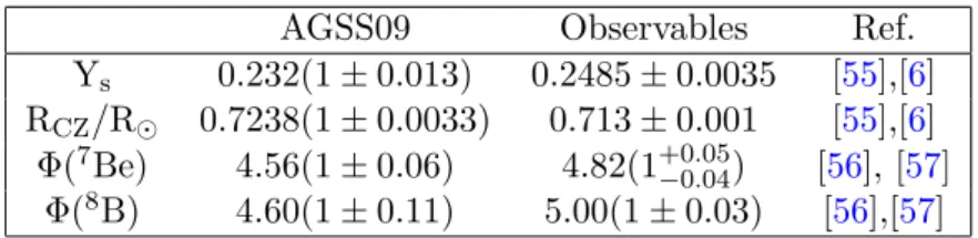
0.5 1.0 1.5 2.0 2.5 3.0 3.5 4.0 -15

-14 -13 -12 -11 -10 -9

Log₁₀(mf/eV) Log10(ϵ)

RG WD HB

Sun

Magnetic Trapping

XENON10

Figure 2. Trapping of MCPs inside the Sun due to a magnetic field. For MCPs with large masses trapping becomes more effective and our assumptions of free streaming break down.

equals the number density of electrons, and E

(3/2)T is the energy of the emitted MCPs, where the approximation holds for MCPs produced by typical thermal plasmons.

In terms of this cross section, the mean free path reads λ = 1

2σ

n

, (3.9)

where we took into account electrons and protons by setting n

n

. Comparing this to the radius of the Sun R

7

10

cm, we obtain that scattering of MCPs only becomes significant for

> 4.6

10

. (3.10)

Minicharged particles can also be trapped by magnetic fields if they force the MCPs on a Larmor radius that is of the order of the radius of the Sun. Even MCPs that leave the Sun might reenter while following a magnetic field line.

The Larmor radius r

can be found to be

r

= γβm

eB =

E

m

eB , (3.11)

where we take B

1 G as the polar magnetic field of the Sun [64,

γ = E/m

and β = p/E are the usual parameters of a Lorentz boost with energy E and momentum p. A comparison of this radius with 10 times the Sun’s radius leads to a trapping for low-mass MCPs of the order

8.8

10

. (3.12)

The exact behavior with mass compared to the bound from fig.

is shown in fig.

For values below the red dot-dashed curve, our assumption of free-streaming is valid. For

larger , our assumptions are invalidated and more intricate computations have to be done.

Note, however, that such large- MCPs change the Sun’s evolution even more drastically.

Hence, our results tentatively hold for larger couplings as well.

3.4 Analytical estimate

An analytical bound on MCPs from the Sun has been derived before in ref. [24] by using a maximum excess luminosity for MCPs L

of L

/L

< 10%, thereby obtaining a limit < 6

10

for m

= 0 eV. Interestingly, this bound is already very close to the one obtained by RGs and HB stars (both < 2

10

[14]), where also an energy sink of 10% of the star’s created energy was assumed.

That the RGs and HB stars are not much better in constraining MCPs can be un- derstood from the structure of the energy-loss rate eq. (3.4). For m

= 0 the rate is proportional to T

ω

T

n

. Whereas the temperatures of the Sun, RGs and HB stars are not very different (T

/T

8), the densities vary by orders of magni- tude ω

/ω

100. While this difference leads to a higher emissivity of the denser stars, RGs and HB stars are more luminous than the Sun as well. This can be taken into account by comparing the energy creation rate per unit mass

. Dividing by the local density,

becomes proportional to T

alone. Using a maximum energy loss for HB stars of

< 10 erg/s/g, an average temperature profile

= 0.44 [62], and a maximum energy loss of the Sun of

< 0.2 erg/s/g, we obtain that the bounds from [14,

behave like

/

3, as seen above.

Conversely, a luminosity constraint for the Sun of L

< 1% L

, which corresponds to an order of magnitude improvement over the assumption by ref. [24], allows us to obtain similar bounds for RGs, HB stars and the Sun. We show in sec.

that such an improvement can actually be obtained by carefully studying the SSMs.

4 Statistical method

We follow the statistical procedure that was introduced in ref. [53] and applied in ref. [26]

to obtain constraints on axions and massive hidden-photons. We construct a χ

-function that is used to quantify the quality of the solar models with respect to the 34 observables described in sec.

using a method that is equivalent to a covariance matrix. To do so, we use the formula described in ref. [66]

χ

= min

{ξ_I}



 X

Q

δ

I

ξ

C

U

2

+

I

ξ





, (4.1)

where δ

= 1

obs

is the relative difference between the model and observational data, U

corresponds to the uncorrelated experimental errors and C

are the correlated theoretical uncertainties that are calculated by propagating the uncertainties of the input parameters I of the SSMs to the observables, as in ref. [53]. These input parameters are:

age, diffusion coefficients, luminosity, opacity and six astrophysical S-factors for the most relevant nuclear reactions.

In this method, ξ

is a random variable with a standard normal distribution, and a shift ξ

C

is introduced to account for the correlations of the errors. This shift can be understood as a correction to the theoretical predictions of Q

when the input parameters are varied. The penalty term

I

ξ

is included in the χ

to account for

Figure 3. Energy-loss distribution of spheres with radius r for different values ofm_f. The left panel corresponds to the case where 2m_f < ω_p so that the emission is not suppressed at least somewhere inside the Sun. The right panel corresponds to the suppressed emission 2m_f > ω_p.

the situation where the input parameters are away from their expected values, and thus, unrealistic in terms of the solar evolution. The values of ξ

that minimize the χ

are called the pulls and they give information about tensions between parameters and data (e.g. it is not possible to change the luminosity and the opacity in different directions).

As we do not want our results to be affected by the solar abundance problem (see sec.

2.2), we construct as a reference a new solar model by letting the composition free, within

realistic input parameters, in order to minimize the χ

-function and to best reproduce the observations. Following ref. [53], we group the elements into two different classes,

(Mg, S, Si, Fe) and

(C, N, O, Ne). We vary them with a multiplicative factor (1 + δ

) and look for the values of δ

and δ

that minimize the χ

function.

For the case without dark emission, the solar model thus obtained is called the

[26,

For the case with MCP emission, we proceed in a similar way. We fix an MCP mass m

and then, for different minicharges , calculate the χ

-function letting the composition free as before. Comparing the resulting χ

-values, we can obtain a bound in the (, m

) plane as is shown in sec.

while fixing m

, this corresponds to a χ

with two degrees of freedom.

As has been pointed out in ref. [26], this procedure is valid when the emission depends only on the stratification of the temperature and mass density in the solar interior and not on its detailed composition. This is the case for MCPs as can be seen from the analytical emission rates in eqs. (3.4) and (3.7). Therefore, our results will not depend on the composition, and we present all results using the more recent composition compilation AGSS09.

5 Minicharged particles in the Sun

We now include the energy loss of MCPs in the SSMs. The MCPs change the internal

structure of the Sun, especially the temperature and density profile. In fig.

the exotic energy-loss distribution as a function of the solar radius for different m

with

= 2.2

10

and in fig.

we show the values of ω

as a function of the solar radius. For

m

= 0, on-shell plasmon decay is possible everywhere inside the Sun because 2m

< ω

is always fulfilled. For m

> 0, less dense regions do not allow for on-shell decay anymore

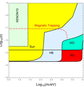
Figure 4. Solar plasma frequency as a function of the solar radius for the SSM (= 0).

and the weaker off-shell decay occurs. Hence, the emission rate is strongly suppressed for larger radii.

On-shell emission is completely suppressed when 2m

> ω

everywhere inside the Sun.

The maximum value for the plasma frequency of the SSMs, we consider in the following, peaks at around ω

290 eV such that for m

175 eV only off-shell decay is possible.

For m

= 150 eV, fig.

shows a two-peaked structure. The reason for this is that quasi on-shell emission occurs in a small sphere around the core of the Sun. Here, the emission rate is dominated by the flank of the quasi-particle Breit-Wigner profile which rises quickly when ω

approaches 2m

.

As apparent from fig.

m

lead to different energy-loss distribu- tions and, thus, different results for the solar structure. To show the different effects, in figs.

and

we have plotted the resulting sound speed profiles and neutrino fluxes for MCP models with four different masses. The results are the outputs of AGSS09 when including MCPs and before the variation of the composition. The results for Y

and R

are not presented in this paper because they do not change substantially for the range of considered here. They will contribute to the global value of the χ

but they are not significant in giving constraints on .

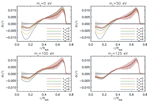
5.1 Sound speed profiles

The effect of the radial distribution of the energy-loss on the sound speed profile can be understood by comparing MCP models with equal minicharges but different masses. For small values of m

, the deviation of the profile with energy-loss from the Standard Solar Model without extra energy-loss is apparent all along the sound speed profile (see fig.

For larger masses m

, the total energy-loss is reduced so that the change in the sound speed profile becomes less relevant. Moreover, the MCP emission is more localized in the inner part of the Sun where on-shell emission still takes place, so that the sound speed profile is altered more drastically in the inner region.

5.2 Neutrino fluxes

When we calculate solar models with exotic energy-loss, we observe changes on the neu-

trino fluxes as can be seen in fig.

in the following way: When we add some extra energy-loss to a solar model, we need to

Figure 5. Sound speed profiles of AGSS09. Each of the panels represents one value formf. Grey shade corresponds to the observational errors and red shade to the theoretical ones.

increase the energy production through nuclear reactions in order to reach the observed solar luminosity (L

= L

L

) resulting in an increase of the neutrino fluxes.

This situation should not be confused with the one described in ref. [67] (a case without exotic energy losses) where it is shown that the

neutrino flux depends on a negative power of the temperature. The difference is that in the situation of ref. [67], the condition to fulfill is L

= L

, so that when neutrinos are neglected all the energy created through nuclear reactions contributes to the solar luminosity. Then, if we increase the temperature, the ratio between the ppI process of the pp-chain and the more energetic ppII process will change favoring the latter. Hence, the

production decreases to maintain L

= L

. In our work, we fulfill L

+ L

= L

instead so that the nuclear energy has to increase in order to account for the extra energy loss.

The reaction rates of

Be + e

Li + ν

and

B

Be + e

+ ν

increase strongly with rising temperature making these neutrino fluxes very sensitive to temperature changes.

Their emissivity of high energy neutrinos can be measured experimentally and poses an independent probe of the solar interior.

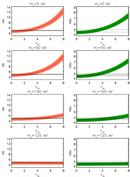
In fig.

B (left panel) and

Be (right panel) neutrino fluxes as a function of for models with different masses. For the cases with m

= 0, 50, 100 eV, both neutrino fluxes increase with increasing and, hence, energy-loss. This shows that in the regions where those nuclear reactions take place the temperature is higher than the SSM.

The case m

= 125 eV is rather peculiar. In fig.

the -range that we have plotted, meaning that the energy-loss rate is too low to produce

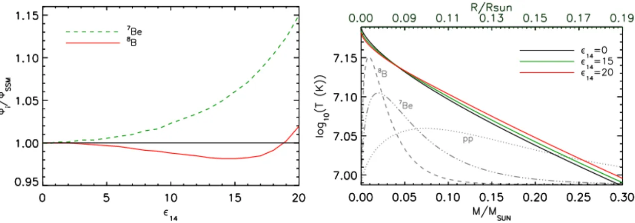
noticeable changes in the Sun. In fig.

(left panel), we extend the parameter space and

show the relative variation in the range of where the changes are significant. We can

observe that the trend of the

B flux differs from the cases seen before. The

B flux

initially decreases with while the flux of

Be increases with it.

Figure 6. ⁷Be (right panel) and ⁸B (left panel) neutrino fluxes as a function of ₁₄ =×10¹⁴. Each row represents one value form_f. Dashed lines correspond to the observational errors whereas the colored regions correspond to theoretical errors. The fluxes are in 10⁹cm⁻²s⁻¹for Φ(⁷Be) and 10⁶cm⁻²s⁻¹ for Φ(⁸B).

This interesting behavior can be explained if we study how the temperature profile in

the interior behaves for cases with different . In the right panel of fig.

profile for three different cases with = 0, = 15

10

(∼ 0.1 L

) and = 20

10

(∼ 0.2 L

). In the interior (r < 0.08 R), the temperature decreases when we include

extra energy-losses, while in the rest of the Sun the temperature increases. The change

in the temperature profile results in different flux variations depending on where the

reactions take place. In the right panel of fig.

distribution as a function of radius of the fluxes Φ(pp), Φ(

B) and Φ(

Be). We see that

Φ(

B) is localized in the region where the temperature decreases with increasing energy-

loss, which explains why the flux initially decreases with . On the other hand, the Φ(

Be)

flux lies in both (increasing and decreasing temperature) regions. The result is going to be

Figure 7. Left panel: Relative neutrino flux of them_f = 125 eV model with respect to AGSS09 as a function of₁₄. The green dotted line corresponds to the⁷Be neutrino flux and the solid red line to the⁸B neutrino flux. Right panel: Temperature profile for the model withm_f = 125 eV for three different values ofas a function of mass and radius. The normalized probability distribution of the production as a function of radius for the different neutrino fluxes are given by grey dotted, dashed and dash-dotted lines.

a combination of the decrease of the

Be production rate in the inner part and the increase of the production of neutrinos in the more exterior part. In this particular situation, this results in an increase of the

Be neutrino production as a function of . In general, it is hard to predict the behavior of the neutrino fluxes for highly localized exotic emission since the variation depends on more factors than just the temperature profile (abundance of protons,

He equilibrium abundance, etc.).

Finally, we would like to mention that some works, as e.g. ref. [67], show that the neutrino fluxes can be expressed as power-laws of the central temperature of the Sun (Φ

T

). In contrast, in this work, we have shown that this relation should be used with great care because it does not apply to all situations. We show that one should take the whole temperature profile into consideration and not just focus on the central temperature of the Sun.

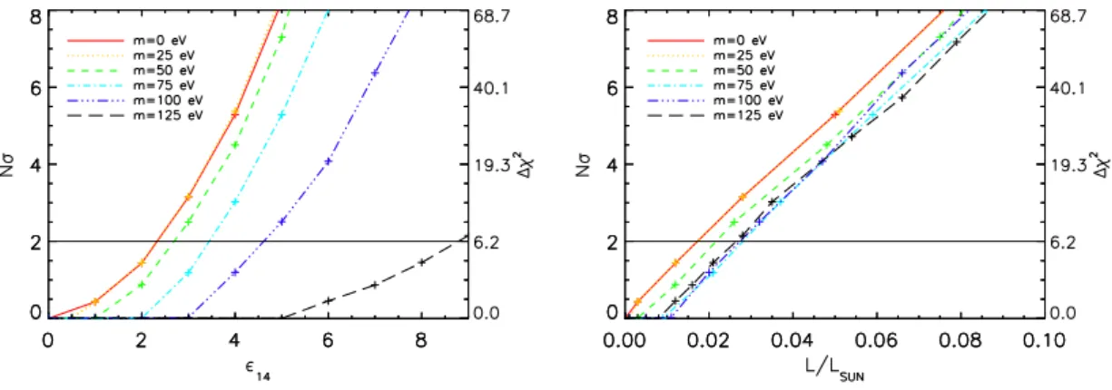
6 Results

We have calculated the χ

-function for different MCP masses varying the composition as described in sec

χ

= 38.5 using 34 observables, which is also the minimal χ

for almost all the masses. For some values of m

, however, the minimum is not exactly at = 0 (SSM) but close to it, which could be due to some small tensions between the sound speed profile and the radius at the convective zone. However, these deviations are not statistically significant. Hence, we come to the conclusion that for all the models, the presence of MCPs does not improve the agreement of the models with the observations. On the other hand, when the energy-loss starts being important, χ

grows smoothly and we use this function to limit an MCP contribution.

In this paper, we derive an upper limit at 2σ CL in the (m

, )-plane. The confidence level can be determined with ∆χ

= χ

, where for a two degrees of freedom problem

∆χ

= 2.3, 6.2, 11.8, 19.3 correspond to confidence levels of N σ = 1, 2, 3, 4 σ. In fig.

plot the resulting values of N σ as a function of (left panel) and the exotic luminosity

Figure 8. N σ and ∆χ² as a function of₁₄ (left panel) and MCP luminosity L_MCP/L (right panel) for models with differentm_f.

m

(eV)

10

at 2σ L

/L

(%) m

(eV)

10

at 2σ L

/L

(%)

0 2.2 1.5 150 460 -

25 2.2 1.5 175 460 2.3

50 2.6 2.0 200 500 2.4

75 3.4 2.7 316 600 2.3

100 4.5 2.6 1000 1090 2.3

125 8.7 2.6 3160 7720 2.8

Table 2. Bounds onat 2σCL and the corresponding luminosity for different values ofmf. For mf= 150 eV, we take the limit of mf = 175 eV (see the main text).

(right panel). The bounds at 2σ and the corresponding exotic luminosity are summarized in tab.

We find that the 2σ bounds on become weaker for larger masses. That is because the MCP emission is reduced and more localized in the inner part as it was shown in fig.

However, when we consider this bound as a function of luminosity (right panel of fig.

can see that for all the cases this luminosity is in a similar range (L

/L

= 1.5

2.7%).

This dispersion in luminosity at 2σ is related to the fact that the distribution of energy-loss in the Sun is different for each of the masses which will translate into different effects on the structure of the Sun. That means that we cannot use a general value for the exotic luminosity to constrain the MCPs parameter space because the luminosity depends on the exact emission of the particle-model studied, as it was already mentioned in ref. [26].

While fig.

shows the MCP models where 2m

< ω

at least in some parts of the Sun so that stringent limits on can be achieved, the energy-loss is strongly suppressed everywhere for 2m

> ω

where only off-shell emission is present. This suppression will lead to bounds that are much weaker.

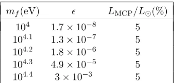
Using the statistical method described above, we compute bounds on MCPs until

3160 eV. For larger masses, MCPs from the Sun are already disfavored so that it suffices

to analytically estimate the behavior of the bound. For m

> T , the emission rate (3.7)

approximately scales like m

exp(−2m

/T ). Conservatively assuming an emission rate of

5%L

, we obtain the values in tab.

for m

> 3160.

m

(eV) L

/L

(%) 10

1.7

10

5 10

1.3

10

5 10

1.8

10

5 10

4.9

10

5

10

3

10

5

Table 3. Analytical estimate for the bound onform_f >3160. We assume an exotic luminosity of 5%L.

Finally, a comment on the model with m

= 150 eV. This case is peculiar because of the two-peaked structure that is present in the center (see fig.

very narrow which resulted into convergence problems of the solar models. In order to be conservative, for m

= 150 eV we use the bound obtained for the model m

= 175 eV corresponding to a value of = 4.6

10

. This is warranted because the emission rate of the m

= 150 eV model is stronger than the emission rate for m

= 175 eV (see fig.

The limit on would, hence, be stronger for m

= 150 eV than the value adopted here.

7 Discussion and summary

Light, weakly-interacting particles can be well constrained by astrophysical sources. For a global picture, we present in tab.

limits on various characteristics of light particles that have been mainly obtained from the energy-loss argument. In the table, we also updated the result for MCPs from the Sun and the constraint on the magnetic moment of the neutrino. In general, constraints derived from the Sun are much weaker than those obtained from red giants, horizontal branch stars, white dwarfs or supernovae because of their more extreme environments. This argument is confirmed by the new limit on the neutrino magnetic moment that we have derived using the same method as for MCPs (see app.

from more massive objects.

To derive this limit, we use the statistical approach described in ref. [26] to compare the results of solar simulations with the emission of minicharged particles to models without a contribution from minicharged particles. Using helioseismology and neutrino data, we are able to derive a limit < 2.2

10

(95% CL) on minicharged particles with masses m

< 25 eV, which corresponds to a maximum excess luminosity of L

/L

< 1.5%. We also computed the behavior of this bound for higher masses of the MCP using on-shell and off-shell plasmon decay. The results are presented in fig.

giving the most comprehensive summary on the available parameter space for MCPs with and without a hidden photon.

Our low-mass bound (m

= 0) is close to the ones derived from red giants and horizontal

branch stars. The importance of the Sun for MCPs can be understood by noting that the

emission rate per unit mass of MCPs is mostly sensitive to the temperature but not to

the density. Moreover, the luminosity constraint for the Sun is more stringent, but also

better understood: whereas the usual assumption of L

/L

< 10% is rather ad

hoc, the result of this paper makes use of the well studied environment of the Sun to

yield L

/L

< 1.5%. This statement also contains statistical information that is not

available for other stars.

MCPs () L-HP κm

[eV] T-HP κ Sun 2.2

10

4.2

10

[21] 2

10

[23]

Red Giant 2

10

[14,

2.1

10

[21] 9

10

[23]

Horizontal Branch 2

10

[14,

1

10

[21,

1

10

[23]

White Dwarf 1.5

10

[14] - -

Supernova 1987a 10

> > 10

[18] - - µ

/µ

g

[GeV

] g

Sun 1.4

10

(App.

4.1

10

[26] 2.3

10

[28]

Red Giant 4.5

10

[20] 0.66

10

[22] 4.3

10

[20]

Horizontal Branch 1.4

10

[24] 0.66

10

[22] 4.3

10

[20]

White Dwarf 5

10

[68] 1.5

10

[69]

2.8

10

[70]

Supernova 1987a 4

10

[19] 5.3

10

[71]

-

†These bounds are not derived directly from the energy-loss argument

Table 4. Summary of bounds on various light, weakly-interacting particles: The minicharge of minicharged particles (MCPs), the product of kinetic mixing and mass κm_V of longitudinal hidden photons (L-HP), and the kinetic mixing κ of transversal hidden photons (T-HP), the diagonal magnetic momentsµ_ν of Dirac neutrinos, the ALP-photon couplingg_aγand ALP-electron couplingg_aefrom various astrophysical sources. The bounds for MCPs are valid roughly up to half the plasma frequency of the source. For L-HP the bound becomes less strict already before the mass of the hidden photon reaches the plasma frequency. For T-HP we quote the most stringent values. Limits on neutrino magnetic momentsµν were again obtained from plasmon decay. Note that from red giants the best 68% CL bound has been found in refs. [72,73]. The presented value forµν from the Sun is a new limit obtained by using the same statistical method as for MCPs (see appendix). Note that the bound on the ALP photon coupling from white dwarfs does not rely on the cooling argument but on spectral distortion. The bound from the supernova 1987a is derived from the non-observance of a gamma-ray signal in the GRS instrument and is valid for very small masses ma<4.4×10⁻¹⁰eV [71].

We would also like to highlight, that for certain parameters of MCP emission, it is possible to increase the neutrino emission of

Be while at the same time decreasing the emission of

B. This interesting feature arises, because for large MCP masses the emission is confined to a small region around the center of the Sun.

Since the Sun is our closest astrophysical object, future improvement in our available data and understanding are to be expected. Interestingly, also dark matter experiments are close to being sensitive to tiny fluxes of MCPs from the Sun. The new data to come will allow us to either further constrain the emission of MCPs from the Sun or to ultimately encounter new signs of physics beyond the Standard Model.

Acknowledgments

We are indebted to Aldo Serenelli and Javier Redondo for a series of insightful remarks,

and to Georg Raffelt for all the support during this project. NV thanks Francesco Vil-

lante and Jordi Isern for their useful advice. HV would like to thank Ignacio Izaguirre

for helpful suggestions and Sacha Davidson for a useful correspondence. NV acknowl-

edges funding support from ESP2013-41268-R (MINECO), 2014SGR-1458 (Generalitat

de Catalunya) and the MICINN grant AYA2011- 24704. HV acknowledges support by the

Mass m

[GeV] minicharge Mass m

[GeV] minicharge

< 84 > 2/3 < 0.1 > 0.01

< 45 > 0.24 < 0.01 > 3

10

< 13 > 0.2 < 2

10

> 10

< 10 > 0.09 < 1

10

> 6

10

< 5 > 0.08 < 2

10

> 3

10

< 1 > 0.03

Table A. Collider constraints according to refs. [14,31].

Deutsche Forschungsgemeinschaft (DFG) under Grant No. EXC-153 (Excellence Cluster

”Universe”), and by the Research Executive Agency (REA) of the European Union under Grant No. PITN-GA-2011-289442 (FP7 Initial Training Network Invisibles).

A Collider constraints on minicharged particles

We updated the collider constraints in fig.

on minicharged particles including the con- straints by both ref. [31] and ref. [32]. The values are given in tab.

B Neutrino magnetic moments

Using the same method as for MCPs, we can also derive a bound on neutrino magnetic moments. The emission rate of massless neutrinos via plasmon decay is again given by

Q

= 2 2π

Z ∞ 0

dkk

ωΓ

e

1 , (B.1)

where the decay rate is [62]

Γ

= µ

24π

Z

ω ω

. (B.2)

Here µ

is the neutrino magnetic moment, which we want to constrain. Note that the rate depends on ω

instead of ω

as was the case for MCPs. This stronger dependence of the density makes the Sun a weaker probe than the more dense RGs and HB stars.

The obtained bound is

µ < 1.4

10

µ

, (B.3)

which corresponds to a luminosity of L

< 1.3% L

. This limit is better than previous estimates from the Sun [24] but worse than the values obtained from RGs in ref. [20].

References

[1] BorexinoCollaboration, O. Yu. Smirnov et al.,Measurement of neutrino flux from the primary proton–proton fusion process in the Sun with Borexino detector,

[arXiv:1507.02432].

[2] SNOCollaboration, Q. R. Ahmad et al.,Direct evidence for neutrino flavor transformation from neutral current interactions in the Sudbury Neutrino Observatory,Phys. Rev. Lett.89 (2002) 011301, [nucl-ex/0204008].

[3] J. Christensen-Dalsgaard,Helioseismology, Reviews of Modern Physics74 (2002) 1073–1129, [astro-ph/0207403].

[4] J. N. Bahcall, M. H. Pinsonneault, and S. Basu,Solar Models: Current Epoch and Time Dependences, Neutrinos, and Helioseismological Properties,ApJ555(2001) 990–1012, [astro-ph/0010346].

[5] A. M. Serenelli, W. C. Haxton, and C. Pe˜na-Garay,Solar Models with Accretion. I.

Application to the Solar Abundance Problem,ApJ743(2011) 24, [arXiv:1104.1639].

[6] S. Basu and H. M. Antia,Constraining Solar Abundances Using Helioseismology,ApJL606 (2004) L85–L88, [astro-ph/0403485].

[7] A. M. Serenelli, S. Basu, J. W. Ferguson, and M. Asplund,New Solar Composition: The Problem with Solar Models Revisited,ApJL705(2009) L123–L127, [arXiv:0909.2668].

[8] R. D. Peccei and H. R. Quinn, CP Conservation in the Presence of Instantons,Phys. Rev.

Lett.38(1977) 1440–1443, [inSPIRE].

[9] P. Galison and A. Manohar,Two Z’s or not two Z’s?,Phys. Lett.B136(1984) 279, [inSPIRE].

[10] B. Holdom,Searching forCharges and a New U(1),Phys.Lett.B178(1986) 65, [inSPIRE].

[11] L. B. Okun,Limits of electrodynamics: paraphotons?,Sov. Phys. JETP56(1982) 502. [Zh.

Eksp. Teor. Fiz.83,892(1982)], [inSPIRE].

[12] R. Foot, G. C. Joshi, H. Lew, and R. R. Volkas,Charged neutrinos?,Mod. Phys. Lett.A5 (1990) 95. [Erratum: Mod. Phys. Lett.A5,2085(1990)], [inSPIRE].

[13] J. Isern, M. Hernanz, and E. Garcia-Berro,Axion cooling of white dwarfs, ApJL5(1992) 392.

[14] S. Davidson, S. Hannestad, and G. Raffelt,Updated bounds on milli-charged particles, Journal of High Energy Physics5(2000) 3, [hep-ph/0001179].

[15] Isern, J. and Garc´ıa-Berro, E. and Torres, S. and Catal´an, S.,Axions and the Cooling of White Dwarf Stars ApJL(2008) 682.,[arXiv:0801.1527].

[16] Isern, J. and Garc´ıa-Berro, E. and Althaus, L. and C´orsico, A. H,Axions and the pulsation periods of variable white dwarfs revisited A& A(2010) 512.,[arXiv:1001.5248].

[17] M. M. Miller Bertolami, B. E. Melendez, L. G. Althaus, and J. Isern,Testing Fundamental Particle Physics with the Galactic White Dwarf Luminosity Function, [arXiv:1410.1677].

[ASP Conf. Ser.493,133(2015)].

[18] R. N. Mohapatra and I. Z. Rothstein,Astrophysical constraints on minicharged particles, Phys. Lett.B247(1990) 593–600, [inSPIRE].

[19] A. Ayala, J. C. D’Olivo, and M. Torres,Bound on the neutrino magnetic moment from chirality flip in supernovae,Phys. Rev.D59 (1999) 111901, [hep-ph/9804230].

[20] N. Viaux et al.,Neutrino and Axion Bounds from the Globular Cluster M5 (NGC 5904), Physical Review Letters111(2013) 231301, [arXiv:1311.1669].

[21] J. Redondo and G. Raffelt,Solar constraints on hidden photons re-visited,JCAP1308 (2013) 034, [arXiv:1305.2920].

[22] A. Ayala, I. Dominguez, M. Giannotti, A. Mirizzi, and O. Straniero,Revisiting the bound on axion-photon coupling from Globular Clusters,ArXiv e-prints(2014) [arXiv:1406.6053].

[23] H. An, M. Pospelov, J. Pradler, and A. Ritz,Direct Detection Constraints on Dark Photon Dark Matter,Phys. Lett.B747(2015) 331–338, [arXiv:1412.8378].

[24] G. G. Raffelt,Limits on neutrino electromagnetic properties - an update.,Phys Rep320 (1999) 319–327, [inSPIRE].

[25] H. An, M. Pospelov, and J. Pradler,New stellar constraints on dark photons,Phys. Lett.

B725(2013) 190–195, [arXiv:1302.3884].

[26] N. Vinyoles, A. Serenelli, F. L. Villante, S. Basu, J. Redondo, and J. Isern,New axion and hidden photon constraints from a solar data global fit,JCAP10(2015) 15,

[arXiv:1501.01639].

[27] J. Redondo,Helioscope Bounds on Hidden Sector Photons,JCAP0807 (2008) 008, [arXiv:0801.1527].

[28] J. Redondo,Solar axion flux from the axion-electron coupling,JCAP1312(2013) 008, [arXiv:1310.0823].

[29] H. Vogel and J. Redondo,Dark Radiation constraints on minicharged particles in models with a hidden photon,JCAP1402 (2014) 029, [arXiv:1311.2600].

[30] PlanckCollaboration, P. A. R. Ade et al.,Planck 2015 results. XIII. Cosmological parameters, [arXiv:1502.01589].

[31] S. Davidson, B. Campbell, and D. C. Bailey,Limits on particles of small electric charge, Phys. Rev.D43(1991) 2314–2321, [inSPIRE].

[32] S. Davidson, S. Hannestad, and G. Raffelt,Updated bounds on millicharged particles, JHEP (2000) 003, [hep-ph/0001179].

[33] S. Dubovsky, D. Gorbunov, and G. Rubtsov,Narrowing the window for millicharged particles by CMB anisotropy,JETP Lett. 79(2004) 1–5, [hep-ph/0311189].

[34] J. Jaeckel, M. Jankowiak, and M. Spannowsky,LHC probes the hidden sector,Phys. Dark Univ.2(2013) 111–117, [arXiv:1212.3620].

[35] A. Prinz, R. Baggs, J. Ballam, S. Ecklund, C. Fertig, et al.,Search for millicharged particles at SLAC,Phys.Rev.Lett. 81(1998) 1175–1178, [hep-ex/9804008].

[36] A. Badertscher, P. Crivelli, W. Fetscher, U. Gendotti, S. Gninenko, et al.,An Improved Limit on Invisible Decays of Positronium,Phys.Rev.D75 (2007) 032004, [hep-ex/0609059].

[37] S. Gninenko, N. Krasnikov, and A. Rubbia,Search for millicharged particles in reactor neutrino experiments: A Probe of the PVLAS anomaly,Phys.Rev.D75(2007) 075014, [hep-ph/0612203].

[38] D. E. Soper, M. Spannowsky, C. J. Wallace, and T. M. P. Tait,Scattering of Dark Particles with Light Mediators,Phys. Rev.D90 (2014), no. 11 115005, [arXiv:1407.2623].

[39] H. An, M. Pospelov, and J. Pradler,Dark Matter Detectors as Dark Photon Helioscopes, Phys. Rev. Lett.111(2013) 041302, [arXiv:1304.3461].

[40] A. Haas, C. S. Hill, E. Izaguirre, and I. Yavin,Looking for milli-charged particles with a new experiment at the LHC,Phys. Lett.B746(2015) 117–120, [arXiv:1410.6816].

[41] E. Izaguirre and I. Yavin,New window to millicharged particles at the LHC,Phys. Rev.D92 (2015), no. 3 035014, [arXiv:1506.04760].

[42] B. Holdom,Two U(1)’s and Epsilon Charge Shifts,Phys. Lett.B166(1986) 196, [inSPIRE].

[43] R. Foot and S. Vagnozzi,Dissipative hidden sector dark matter,Phys. Rev.D91 (2015) 023512, [arXiv:1409.7174].

[44] M. Farina,Asymmetric Twin Dark Matter, [arXiv:1506.03520].

[45] C. P. Burgess, J. P. Conlon, L.-Y. Hung, C. H. Kom, A. Maharana, and F. Quevedo, Continuous Global Symmetries and Hyperweak Interactions in String Compactifications, JHEP07(2008) 073, [arXiv:0805.4037].

[46] R. Blumenhagen, G. Honecker, and T. Weigand,Loop-corrected compactifications of the heterotic string with line bundles,JHEP0506 (2005) 020, [hep-th/0504232].