3 4 5
Should metacognition be measured by logistic regression?
6 7 8 9
Manuel Rausch 1,2 and Michael Zehetleitner 1,2 10
11
1 Katholische Universität Eichstätt-Ingolstadt, Eichstätt, Germany 12
13
2 Ludwig-Maximilians-Universität München, Munich, Germany 14
15 16
Correspondence should be addressed at:
17
Manuel Rausch 18
Katholische Univerität Eichstätt-Ingolstadt 19
Psychologie II 20
Ostenstraße 25, "Waisenhaus"
21
85072 Eichstätt 22
Germany 23
Phone: +49 8421 93 21639 24
Email: manuel.rausch@ku.de 25
http://www.ku.de/ppf/psychologie/psych2/mitarbeiter/m-rausch/
26 27
This manuscript was accepted for publication in Consciousness and Cognition. Please cite 28
this work as: Rausch, M., Zehetleitner, M. (2017). Should metacognition be measured by 29
logistic regression? Consciousness and Cognition. 49, 291-312. The final publication is 30
available at http://dx.doi.org/10.1016/j.concog.2017.02.007 31
© 2017. This manuscript version is made available under the CC-BY-NC-ND 4.0 license 32
http://creativecommons.org/licenses/by-nc-nd/4.0/
33 34
Abstract 35
Are logistic regression slopes suitable to quantify metacognitive sensitivity, i.e. the efficiency 36
with which subjective reports differentiate between correct and incorrect task responses? We 37
analytically show that logistic regression slopes are independent from rating criteria in one 38
specific model of metacognition, which assumes (i) that rating decisions are based on sensory 39
evidence generated independently of the sensory evidence used for primary task responses 40
and (ii) that the distributions of evidence are logistic. Given a hierarchical model of 41
metacognition, logistic regression slopes depend on rating criteria. According to all 42
considered models, regression slopes depend on the primary task criterion. A reanalysis of 43
previous data revealed that massive numbers of trials are required to distinguish between 44
hierarchical and independent models with tolerable accuracy. It is argued that researchers 45
who wish to use logistic regression as measure of metacognitive sensitivity need to control 46
the primary task criterion and rating criteria.
47
Keywords: metacognition; metacognitive sensitivity, logistic regression; signal detection 48
theory; type 2 signal detection theory; generalized linear regression, cognitive modelling 49
50
1 Introduction 51
Metacognitive sensitivity, also called type 2 sensitivity or resolution of confidence, refers to 52
the efficiency with which participants’ subjective reports during an experimental task 53
discriminate between correct and incorrect responses in a primary task (Baranski & Petrusic, 54
1994; Fleming & Lau, 2014; Galvin, Podd, Drga, & Whitmore, 2003). It relates to a key 55
aspect of metacognition: If participants possessed any knowledge about their performance in 56
the task, their subjective reports about the task should differentiate between correct and 57
erroneous trials. Consequently, measures of metacognitive sensitivity are relevant for all 58
research areas where quantifying participants’ insight into their task performance is of 59
interest, including consciousness research (Dienes, 2004). Given the theoretical importance 60
of metacognitive sensitivity, a universally accepted measure is desirable. However, various 61
competing measures of metacognitive sensitivity were proposed in the literature:
62
• gamma correlation coefficients (Nelson, 1984), 63
• a’/type 2 d’ (Kunimoto, Miller, & Pashler, 2001) 64
• type-2 receiver operating characteristic ( Fleming, Weil, Nagy, Dolan, & Rees, 65
2010) 66
• meta-d’ (Maniscalco & Lau, 2012) 67
• logistic regression analysis (Sandberg, Timmermans, Overgaard, &
68
Cleeremans, 2010) 69
Logistic regression has been widely used in empirical studies as measure of the association 70
between verbal reports and task accuracy (Rausch, Müller, & Zehetleitner, 2015; Rausch &
71
Zehetleitner, 2014; Sandberg et al., 2010; Siedlecka, Paulewicz, & Wierzchoń, 2016;
72
Wierzchoń, Asanowicz, Paulewicz, & Cleeremans, 2012; Wierzchoń, Paulewicz, Asanowicz, 73
Timmermans, & Cleeremans, 2014). However, while gamma correlations, a’, and meta-d’
74
have been extensively examined using both empirical and analytical methods (Barrett, 75
Dienes, & Seth, 2013; Evans & Azzopardi, 2007; Galvin et al., 2003; Masson & Rotello, 76
2009), the conditions for logistic regression to be an appropriate measure of metacognitive 77
sensitivity have never been systematically investigated.
78
1.1 Logistic regression as measure of metacognitive sensitivity 79
Logistic regression is a specific case of a generalized linear regression model (GLM). In 80
general, it is a method to quantify the relationship between a binary outcome variable and one 81
or several dichotomous or continuous predictors. The standard approach to quantify 82
metacognitive sensitivity by means of logistic regression is to model the probability of being 83
correct in the primary task P(T) as a linear function of a subjective report C, e.g. a confidence 84
judgment or a visibility rating. A linear relationship between predictors and outcome is 85
obtained by transforming the probability of being correct into the logarithm of the odds of the 86
primary response being correct to being incorrect:
87
log( 𝑃(𝑇)
1 − 𝑃(𝑇)) = 𝑎 + 𝑏 ∗ 𝐶 (1)
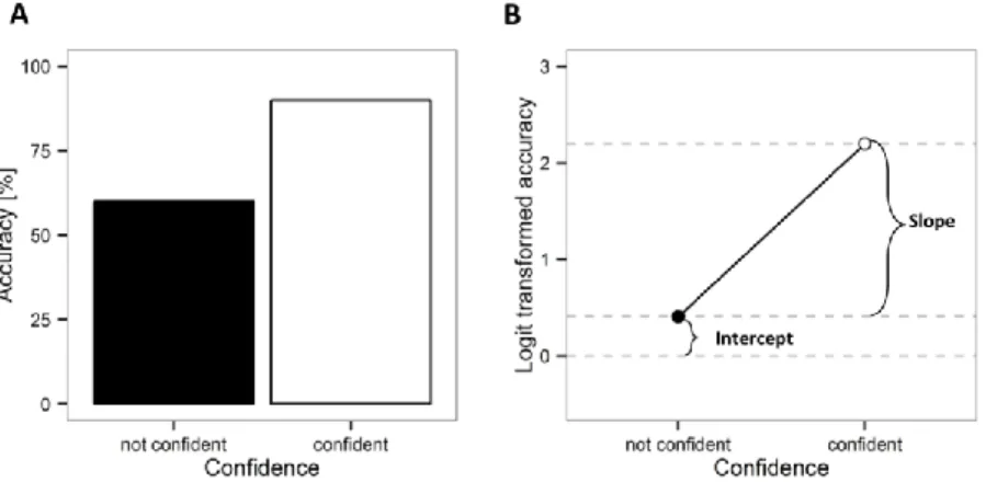
As can be seen from Fig. 1, metacognitive sensitivity is indexed by the slope b of the 88
regression line: the steeper the regression line, the stronger are subjective reports associated 89
with the probability of being correct (Sandberg et al., 2010). Logistic regression is also used 90
to quantify the minimal criteria participants apply when they make a subjective report: The 91
more conservative participants’ reporting strategy is, the better they perform while still giving 92
the lowest possible subjective report. As the intercept a is just the transformed accuracy when 93
the subjective report is zero, it is interpreted as measure of criterion (Wierzchoń et al., 2012).
94
Quantifying metacognition by logistic regression is tempting due to three reasons: First, the 95
hierarchical structure of the data often found in behavioral experiments can be explicitly 96
included into the model by using nested random effects (Sandberg, Bibby, & Overgaard, 97
2013; Siedlecka et al., 2016): For example, two experimental groups with several participants 98
each contributing a number of trials can be described by a random effect of trial nested within 99
a random effect of participant nested within groups. As such an analysis can be conducted on 100
a single trial level without the need for summary statistics to be computed for each 101
participant, logistic regression may also be a promising way to increase statistical power 102
(Sandberg et al., 2010). Second, using random effects allows the data to be unbalanced, i.e.
103
the number of observations can vary between conditions or there can be empty cells in the 104
design matrix (Rausch et al., 2015; Siedlecka et al., 2016). Consequently, slopes on the group 105
level can be obtained even when not all participants made errors in all experimental 106
conditions. This is particularly useful in studies of metacognitive sensitivity because the 107
number of errors may vary heavily between participants and conditions. Finally, it has been 108
argued that logistic regression, unlike SDT-measures, does not make any assumptions about 109
the sources of the evidence involved in making subjective reports (Siedlecka et al., 2016).
110
However, logistic regression as measure of metacognition may also suffer from at least two 111
drawbacks: First, it depends on the assumption that the relation between subjective reports 112
and transformed accuracy is linear. A non-linear relationship implies that there is no single 113
slope of the regression line that could be interpreted as measure of metacognitive sensitivity.
114
A previous analysis suggested non-linear trends between subjective reports and logit- 115
transformed accuracy occur relatively frequently, although there were also some data sets 116
where the assumption of a linear relationship appeared to be justified (Rausch et al., 2015). It 117
should be noted that this critique only applies to rating scales with more than two response 118
options because two data from two response options always can be connected by a straight 119
line.
120
The present analysis explores a potential second and more principal problem of logistic 121
regression: An adequate measure of metacognitive sensitivity should depend exclusively on 122
the amount of evidence available for subjective reports, and should not be confounded by 123
other factors such as rating criteria and response biases (Barrett et al., 2013). Although the 124
distinction between slopes and intercepts appears superficially similar to a separation 125
between metacognitive sensitivity and criteria, it has never been systematically investigated 126
what exactly are the assumptions that have to be fulfilled so that slopes are independent from 127
criteria.
128
1.2 Models of metacognition 129
A systematic investigation of the impact of rating criteria and primary task criterion on 130
logistic regression models requires a mathematically formulated model that accounts for both 131
task responses as well as subjective reports. One of the most prominent models of perceptual 132
decision making under uncertainty is signal detection theory (SDT) (Green & Swets, 1966;
133
Macmillan & Creelman, 2005; Wickens, 2002). Standard SDT applies to tasks where 134
participants are instructed to correctly classify a binary stimulation S. For the purpose of 135
present analysis, it is not relevant whether the two variants of the stimulation are interpreted 136
as signal and noise or as two different stimuli. Each stimulus provides the participants with 137
sensory evidence which of the two response options he or she should select. Participants 138
select their responses based on a comparison of the sensory evidence with a primary task 139
criterion θ. θ represents the degree to which observers tend towards one response option 140
independent of the sensory evidence. Participants respond 0 if the sensory evidence is smaller 141
than θ and 1 otherwise. As there is noise in the system, the sensory evidence is not always the 142
same at each presentation of the stimulus, but instead is modeled as a random sample out of 143
two distributions, one for each variant of S. If the observer’s perceptual system was unable to 144
differentiate between the variants of S, the two distributionswould be identical. The more 145
sensitive the observer is to the stimulus, the greater is the distance d between the centers of 146
the two distributions. This distance d can therefore be interpreted as the ability of the 147
observer’s perceptual system to differentiate between the two kinds of S. The SDT model can 148
be extended to include subjective reports by assuming that task responses and ratings are 149
considered to form an ordered set of responses such as ‘‘I’m sure it’s A’’, ‘‘I guess A’’, ‘‘I 150
guess B’’, ‘‘I’m sure it’s B’’. The different response options are delineated by a series of 151
criteria, c1, c2, …, cn. Participants select one response out of the set of responses by comparing 152
the sensory evidence against the set of criteria. For example, they respond “I guess A” when the 153
sensory evidence falls between that criterion separating the response ‘‘I’m sure it’s A’’ from 154
‘‘I guess A” and that criterion separating “I guess A” from “I guess B”. An important 155
implication of the SDT model is that the full evidence available to task responses is also 156
available to subjective reports (Macmillan & Creelman, 2005), which is why the model is 157
sometimes referred to as “ideal observer model” (Barrett et al., 2013). While the SDT model 158
has been successfully applied to a vast number of different experiments over the last decades 159
(Macmillan & Creelman, 2005; Wickens, 2002), in recent years, more recent experiments 160
both found support for the SDT model (Peters & Lau, 2015), but also situations where 161
subjective reports were not as optimal as expected from SDT (Maniscalco & Lau, 2012, 162
2016) or even better than expected (e.g. Rausch & Zehetleitner, 2016).
163
1.2.1 Hierarchical model 164
Measuring metacognition only makes sense in models where metacognition is not necessarily 165
perfect. For the purpose of the present analysis, we consider two models of how the SDT 166
model can be extended to account for imperfect metacognition, the hierarchical model and 167
the independent model. In both of these two models, the task response is selected by a 168
comparison between sensory evidence and the task criterion, just as in the SDT model. A 169
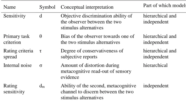
summary of all free parameters of the two models is found in Table 1.
170
TABLE 1 ABOUT HERE 171
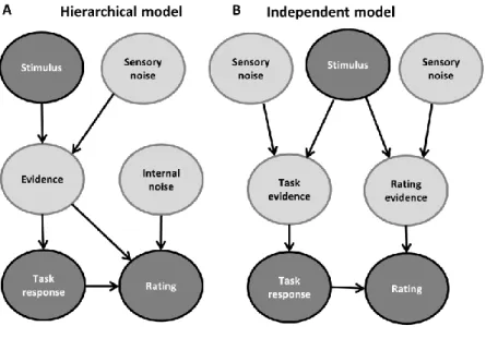
The hierarchical model assumes that the sensory evidence involved in selecting the task 172
response is also involved in selecting a rating category (see Fig. 2a). However, in contrast to 173
standard SDT, it is not assumed that the sensory evidence involved in the task response 174
completely determines the subjective report as well. Instead, the sensory evidence is read out 175
by metacognitive processes, whereas the read-out can be incomplete or distorted (Maniscalco 176
& Lau, 2016). One way to express this mathematically is by assuming that the sensory 177
evidence is overlaid by random additive noise, characterized by its standard deviation, σ (cf.
178
Maniscalco & Lau, 2016). The additive noise σ can interpreted as the degree of distortion 179
between the task process and the metacognitive processes. When the additive noise is absent, 180
the model is identical to the SDT model. For simplicity, we also assume that two rating criteria 181
are placed symmetrically around the primary task criterion θ. The distances of the rating 182
criteria to the task criterion are controlled by the same parameter τ. Conceptually, the spread 183
of rating criteria τ expresses whether subjective reports are made more liberally or more 184
conservatively: When τ is large, the rating criteria are further away from the center of the 185
distribution of sensory evidence. Thus, it is rather unlikely that the sensory evidence is more 186
extreme than the rating criteria; therefore, participants will not often report high confidence.
187
1.2.2 Independent model 188
The present study will propose that logistic regression is closely related to another model of 189
metacognition, the independent model. The independent model is a new variant of so-called 190
dual channel models (cf. Cul, Dehaene, Reyes, Bravo, & Slachevsky, 2009; Maniscalco &
191
Lau, 2016; Rahnev, Maniscalco, Luber, Lau, & Lisanby, 2012). Dual channel models assume 192
that the rating decision does not depend on the sensory evidence considered for the task 193
decision. Instead, rating decisions are based on a second sample of evidence (see Fig. 2b). In 194
contrast to previous flavors of the dual channel model, the independent model discussed here 195
assumes that there is no interaction between the two samples of evidence except that 196
observers know which of two the task responses they choose. As a consequence, they respond 197
high confidence or high visibility when the evidence sampled in parallel confirms the 198
response option they decide for. It is assumed that the distributions from which the parallel 199
samples of evidence are drawn are characterized by the same shape as those distributions of 200
evidence involved in the primary task, except that the distance between the two distributions 201
may deviate from the distance of distributions in the primary task and is denoted by the rating 202
sensitivity parameter dm. Conceptually, the rating sensitivity parameter dm can be interpreted 203
as the amount of evidence available to metacognitive processes that predict whether a 204
decision is correct. Again, we assume that rating criteria are placed symmetrically around the 205
primary task criterion θ, with the distances of the rating criteria to the task criterion controlled 206
by the same parameter τ. The independent model is able to accommodate patterns of data that 207
the hierarchical model struggles to explain: First, the hierarchical model cannot account for 208
participants successfully detecting their own errors (Yeung & Summerfield, 2012). Second, 209
the independent model is able to account for blind insight, e.g. cases when participants 210
perform at chance, but their confidence responses are able to differentiate between correct 211
and incorrect trials (Scott, Dienes, Barrett, Bor, & Seth, 2014). While the hierarchical model 212
achieved better fits to the data than several variants of dual channel models in a metacontrast 213
masking task (Maniscalco & Lau, 2016), the independent model has never been formally 214
assessed with empirical data.
215
1.2.3 Rationale of the present study 216
The present analysis was performed to investigate the eligibility of logistic regression as a 217
measure of metacognition. For this purpose, we computed analytically whether logistic 218
regression slopes depend on parameters conceptually associated with metacognition, i.e. the 219
internal noise σ in the hierarchical model and the distance between distributions dm in the 220
independent model. To test whether logistic regression slopes is biased by task and rating 221
criteria, we varied task bias θ and the spread of rating criteria τ in both models, and 222
investigated the effects on logistic regression slopes. If logistic regression slopes were 223
suitable measures of metacognitive sensitivity, they should be associated with internal noise 224
in the hierarchical model and rating sensitivity in the independent model, and also be 225
independent from task bias and report criteria. To examine the generality of these effects, we 226
also varied the shape of the distributions of evidence generated by the two stimuli. In 227
addition, we varied the link functions, i.e. the transformations to relate subjective reports and 228
task performance. In addition, we performed an analogous analysis to investigate if rating 229
criteria can be assessed by regression intercepts. Finally, data obtained in a low-contrast 230
orientation discrimination task (Rausch & Zehetleitner, 2016) was reanalyzed to investigate if 231
it is possible to differentiate between the hierarchical and the independent model empirically.
232
2 Logistic regression in a hierarchical model of metacognition 233
All analyses were conducted using the free software R (R Core Team, 2014). The analysis 234
code and all reported results are freely available at the Open Science Framework 235
(https://osf.io/72aqe/) to facilitate reproduction of the present study and replication of its 236
results (Ince, Hatton, & Graham-Cumming, 2012; Morin et al., 2012).
237
2.1 Calculation of GLM slopes 238
Analytical closed-form solutions exist for the coefficients of logistic regression when there is 239
one categorical predictor (Lipovetsky, 2015), but this approach generalizes to other GLMs as 240
well. In case of metacognition, the GLM is given by the formula 241
𝑔(𝑃(𝑇 = 1|𝐶)) = 𝑎 + 𝑏 ∗ 𝐶 (2)
with g denoting the link function, which describes the transformation used to relate accuracy 242
and predictors, 𝑃(𝑇 = 1|𝐶) the probability of being correct in the primary task conditioned 243
on participant’s subjective report, a as intercept, b as slope, and C ∈ {0, 1} as subjective 244
report. The intercept is 245
𝑎 = 𝑔(𝑃(𝑇 = 1|𝐶 = 0) (3)
and the slope, which is indicative of metacognitive sensitivity, is given by 246
𝑏 = 𝑔(𝑃(𝑇 = 1|𝐶 = 1)) − 𝑔(𝑃(𝑇 = 1|𝐶 = 0)) (4) Consequently, GLM slopes can be computed analytically in all situations when
247
𝑃(𝑇 = 1|𝐶 = 0) and 𝑃(𝑇 = 1|𝐶 = 1) are known.
248
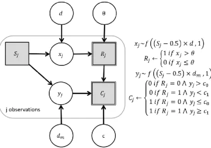
2.2 Model description 249
A graphical model of the hierarchical model is found in Fig. 3. We assume that in each trial 250
of the experiment, participants are presented with one out of two manifestations of the 251
stimulus S ∈ {0, 1} which both occur with the same probability. Participants select a response 252
R ∈ {0, 1} which of the two stimuli was presented. Accuracy of the response T is 1 when 𝑆 = 253
𝑅, and 𝑇 = 0 otherwise. In each trial, participants select a response based on a single sample 254
of sensory evidence x. The sensory evidence x is a random sample out of a distribution that 255
depends on the stimulus. The two distributionscorresponding to the two stimulus variants 256
have the same standard deviation of 1. However, their location depends on the sensitivity 257
parameter d: When 𝑆 = 0, the mean of the distribution is -0.5 d, and when 𝑆 = 1, then the 258
mean of the distribution of evidence is 0.5 d. Participants’ response R is 0 when x is smaller 259
than the primary task criterion θ, and 1 otherwise. The sensory evidence x is overlaid by 260
internal noise, which is randomly sampled out of a distribution with a mean of 0 and a 261
standard deviation determined by the rating noise parameter σ. The sum of x and internal 262
noise is called decision variable z and determines subjective reports by a comparison with 263
rating criteria c0 and c1: When 𝑅 = 1 and the z is greater than the rating criterion c1, then the 264
subjective report C is 1. When 𝑅 = 1 and the z is smaller than the rating criterion c1, then the 265
subjective report C is 0. Likewise, when 𝑅 = 0, than C is 1 if z is smaller than the rating 266
criterion c0, and C is 0 if z is greater than the rating criterion c0. For simplicity, we assume 267
that the distance between θ and c0 is the same as the distance between θ and c1. This distance 268
is controlled by the parameter τ, which reflects the conservativeness of rating criteria. The 269
formulae for computing 𝑃(𝑇 = 1|𝐶 = 0) and 𝑃(𝑇 = 1|𝐶 = 1) in the hierarchical model can 270
be found in the Appendix A.
271
We considered two different distributions of evidence, the Gaussian distribution and the 272
logistic distribution. The Gaussian distribution is often motivated by the central limits 273
theorem and the averaging of many events (DeCarlo, 1998). The logistic distribution can be 274
motivated from Choice Theory (Luce & Suppes, 1965; Macmillan & Creelman, 2005). For 275
most SDT applications, results obtained based on logistic and Gaussian distributions are very 276
similar (DeCarlo, 1998; Wickens, 2002).
277
2.3 Link functions 278
The link function that transforms the probability of being correct to the logarithm of the odds 279
of being correct to being incorrect is called the logit link and is the defining feature of logistic 280
regression. In the present analysis, three different link functions are examined:
281
1) the logit link 282
2) the probit link 283
3) the half-logit link.
284
The logit link was the default choice in previous studies. The probit link was included into 285
the analysis because SDT models can be seen as a subclass of generalized linear regression 286
models where the inverse link function corresponds to the cumulative distribution function of 287
the evidence (Brockhoff & Christensen, 2010; DeCarlo, 1998). Logistic regression assumes a 288
logistic distribution of errors, while probit regression assumes a standard normal distribution 289
of errors. Consequently, it appears necessary to examine if logistic regression is only valid in 290
logistic SDT models, and probit regression in Gaussian SDT models. The adjusted link was 291
proposed as an adjustment in tasks with a finite guessing probability (Brockhoff & Müller, 292
1997). The use of the logit and probit transform implies that the probability of being correct 293
varies between 0 and 1; however, in binary tasks, the probability of being correct is bounded 294
by the guessing probability 0.5 (Rausch et al., 2015). To account for the guessing probability, 295
a link function can be used to ensure that the transformed accuracy is free to vary in the full 296
range between -∞ and ∞. In tasks with two choices, this can be achieved by the adjusted link 297
function g(x) = log((x − 0.5) (1 − x)⁄ ). This function was referred to as half-logit link (cf.
298
Williams, Ramaswamy, & Oulhaj, 2006).
299
2.4 Results 300
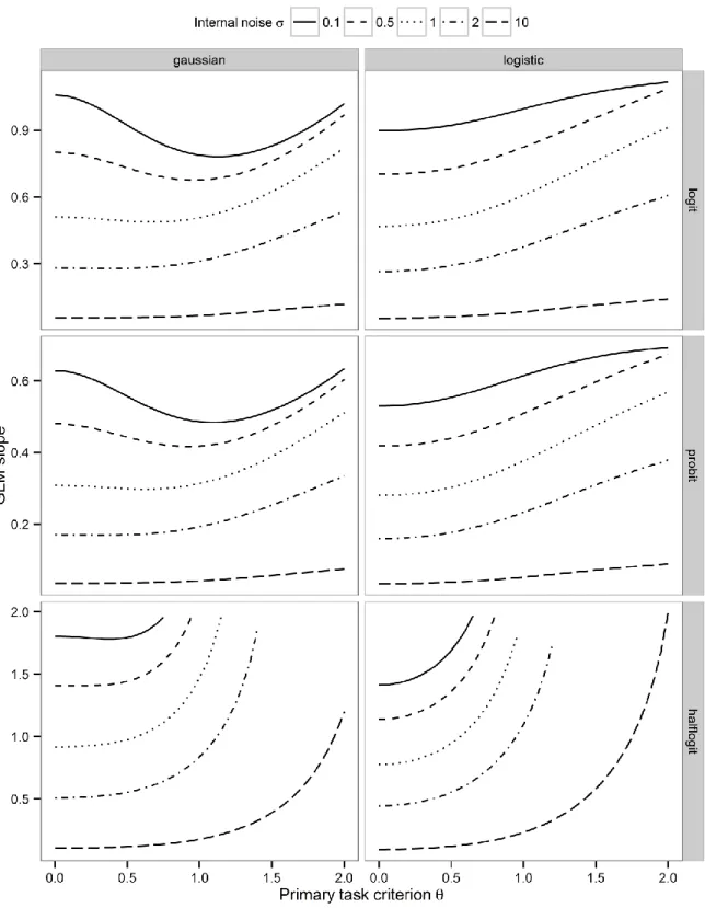
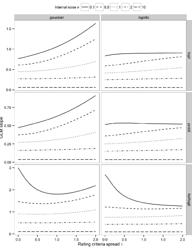
To investigate if GLM slopes are sensitive to metacognition and unbiased by primary task 301
criterion and by rating criteria assuming the hierarchical model, we calculated logistic 302
regression slopes as a function of internal noise σ as well as primary task criterion θ (Fig. 4) 303
and spread of rating criteria τ (Fig. 5). These calculations were repeated using Gaussian and 304
logistic distributions of evidence and with logit, probit, and half-logit link functions.
305
2.4.1 Are GLM slopes sensitive to metacognition?
306
In Fig. 4 and 5, separate lines indicate different degrees of internal noise σ. Greater amounts 307
of internal noise are associated with lower regression slopes at each level of primary task 308
criterion (Fig. 4), and at each level of rating criteria spread (Fig. 5). This pattern holds 309
independently from distributions of evidence and link functions (separate panels of Fig. 4 and 310
5). When the amounts of noise are extreme, i.e. when metacognition is effectively absent, 311
regression slopes also tend towards zero. Overall, GLM analysis is sensitive to metacognition 312
according to the hierarchical model.
313
2.4.2 Do GLM slopes depend on the primary task criterion?
314
As can be seen from each panel of Fig. 4, regression slopes depend heavily on the primary 315
task criterion according to the hierarchical model. The precise form of the relationship 316
between primary task criterion and slopes depends on a complex interaction between the 317
amount internal noise, the shape of the distributions of evidence, and the link functions.
318
When the distributions are logistic, when the half-logit transform is used, or when the internal 319
noise is not small, logistic regression slopes increase monotonously with primary task 320
criterion: Consequently, greater regression slopes are not necessarily due to metacognition, 321
but could also be due to a stronger bias towards one of the task alternatives. However, when 322
Gaussian distributions are assumed and the amount of noise is small, the relationship between 323
regression slopes and primary task criterion is u-shaped: Slopes are maximal when observers 324
are either not biased at all or extremely biased towards one of the task alternatives. Therefore, 325
a primary task criterion may not only increase, but also decrease regression slopes. Overall, 326
regression slopes depend on the primary task criterion, but the direction and magnitude of the 327
effect is strongly dependent on the other model parameters of the hierarchical model.
328
FIG.4 ABOUT HERE 329
2.4.3 Do GLM slopes depend on rating criteria?
330
As can be seen from Fig. 5, logistic and probit regression slopes increase with rating criteria 331
spread τ, i.e. when more conservative rating criteria are set (top and central panels). The 332
relationship between half-logit regression slopes and rating criteria can be u-shaped or 333
decreasing (bottom panels). However, the relationships between slopes and rating criteria are 334
moderated by internal noise as well the shape of the distributions: When the distributions are 335
Gaussian, the effect imposed by rating criteria will be smaller the more internal noise is 336
superimposed on the sensory evidence. When the distributions are logistic, the effect imposed 337
by rating criteria is maximal at medium level of internal noise. Overall, according to 338
hierarchical models, differences between regression slopes can not only be caused by 339
metacognition and task criterion, but also by the way participants set rating criteria. Again, 340
the effect is strongly dependent on the other model parameters of the hierarchical model.
341
FIG. 5 ABOUT HERE 342
2.4.4 Can rating criteria be assessed by regression intercepts?
343
To investigate if regression intercepts are sensitive to rating criteria and independent from 344
metacognition and primary task criterion in the hierarchical model, we calculated intercepts 345
as a function of internal noise σ, primary task criterion θ, rating criteria spread τ, shape of the 346
distributions, and link functions. Consistent across distributions and link functions, intercepts 347
were negatively related to the primary task criterion θ and positively correlated to the internal 348
noise sigma σ (see Supplementary Fig. 1). However, intercepts were only sensitive to the 349
spread of rating criteria τ when the amount of internal noise was low (see Supplementary Fig.
350
2). This means that intercept effects cannot uniquely be attributed to rating criteria, but also 351
to metacognition or due to primary task criterion. Even more, when rating criteria are 352
different between two conditions, it will not be possible to detect the effect using intercepts 353
when the amount of internal noise is high.
354
3 Logistic regression in the independent model of metacognition 355
3.1 Calculation of GLM slopes and link functions 356
Calculation of GLM slopes and link functions were identical to the hierarchical model.
357
3.2 Model description 358
The independent model can be expressed by the graphical model in Fig. 6. It is analogous to 359
the hierarchical model with the following differences: Participants select only the primary 360
task response based on the sensory evidence x. For subjective reports, a second sample of 361
sensory evidence y is created, which is stochastically independent from x. The standard 362
deviation of the distribution of y is assumed to be 1. The location of the distribution of y 363
depends on the stimulus in the current trial as well as on the rating sensitivity parameter dm: 364
When 𝑆 = 0, the mean of the distribution is -0.5 dm, and when 𝑆 = 1, then the mean of the 365
distribution of evidence is 0.5 dm. When 𝑅 = 1and y is greater than the rating criterion c1, 366
then the participant’s subjective report C is 1. When 𝑅 = 1 and y is smaller than the rating 367
criterion c1, then the subjective report C is 0. Likewise, when 𝑅 = 0, the C is 1 if y is smaller 368
than the rating criterion c0, and C is 0 if y is greater than the rating criterion c0. Again, it is 369
assumed for simplicity that the distance between θ and c0 is the same as the distance between 370
θ and c1, controlled by the parameter τ reflecting the conservativeness of rating criteria. The 371
formulae for computing 𝑃(𝑇 = 1|𝐶 = 0) and 𝑃(𝑇 = 1|𝐶 = 1) in the independent model can 372
be found in the Appendix B.
373
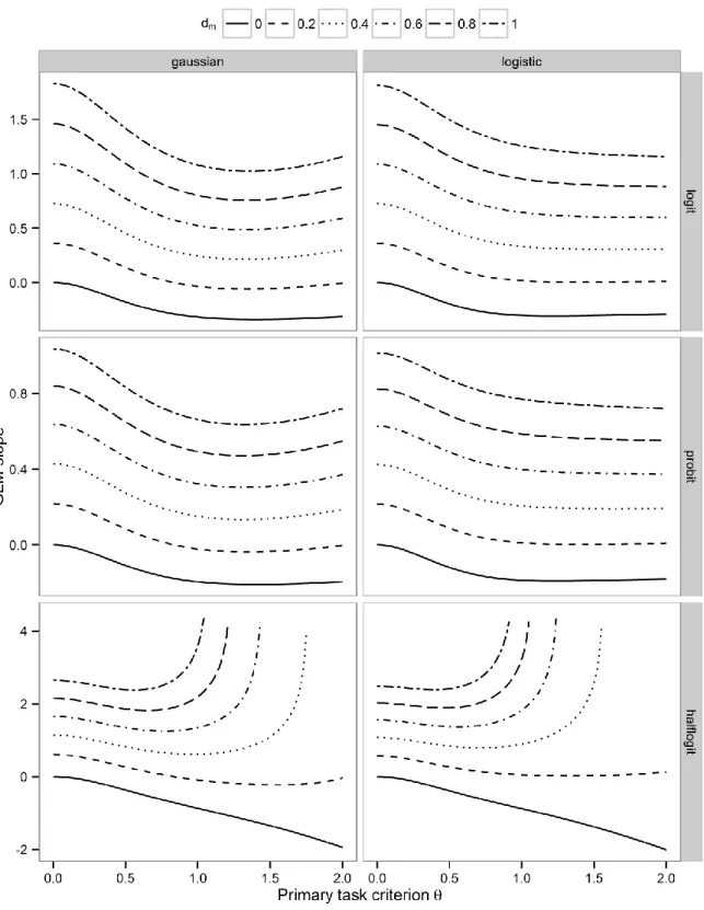
3.3 Results 374
To investigate if GLM slopes are sensitive to metacognition and unbiased by the primary task 375
criterion and by rating criteria according to the independent model, slopes were calculated as 376
a function of rating sensitivity dm as well as primary task criterion θ (Fig. 7) and spread of 377
rating criteria τ (Fig. 8). Again, these calculations were performed using Gaussian and 378
logistic distributions of evidence and using logit, probit, and half-logit link functions.
379
3.3.1 Are GLM slopes sensitive to metacognition?
380
In Fig. 7 and 8, separate lines indicate different degrees of rating sensitivity dm. Greater rating 381
sensitivity was associated with increasing regression slopes at each level of primary task 382
criterion (Fig. 7), and at each level of rating criteria spread (Fig. 8). This pattern holds across 383
the different distributions of evidence and link functions (separate panels of Fig. 7 and 8).
384
When rating sensitivity is 0, i.e. when the sensory evidence available to metacognition does 385
not differentiate between the two stimuli, regression slopes become 0 when observers are 386
unbiased towards the two response options. However, when rating sensitivity is 0 and when 387
there is a bias, the slope will become negative. Overall, these results indicate GLM analysis is 388
sensitive to metacognition in the independent model, but the sign of the slope should not be 389
interpreted without consideration of the primary task criterion.
390
3.3.2 Do GLM slopes depend on the primary task criterion?
391
As can be seen from each panel of Fig. 7, slopes are influenced by the primary task criterion 392
θ according to the independent model as well. While there is always an effect of primary task 393
criterion, direction and magnitude of the effect depends on a complex interaction between the 394
amount of metacognition as indexed by the rating sensitivity dm, the shape of the distributions 395
of evidence, as well as the link functions. When the distributions of evidence are Gaussian 396
and when a probit or logit link function is used, the relationship between primary task 397
criterion θ and slopes appears to be u-shaped and similar across different levels of 398
metacognition: Slopes reach a minimum at medium primary task criterion θ, and increase 399
when θ is either 0 or maximal (see Fig. 7 upper and central panel to the left). When the 400
distributions of evidence are logistic and when a probit or logit link functions is applied, 401
GLM slopes decrease with increasing θ (see Fig. 7 upper and central panel to the right).
402
When the half-logit link function is used, the slopes increase exponentially with θ for 403
medium-to-large rating sensitivities. However, when rating sensitivity is low, slopes decrease 404
with increasing θ. Overall, these observations indicate that slopes as measures of 405
metacognition in the independent model can be biased by the primary task criterion; the kind 406
of bias however depends on the other model parameters as well as on the choice of the link 407
function.
408
FIG.7 ABOUT HERE 409
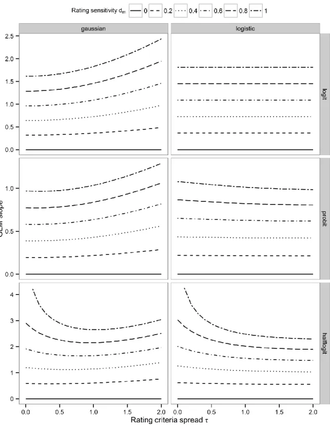
3.3.3 Do GLM slops depend on rating criteria?
410
Fig. 8 shows that GLM slopes are independent from the spread of rating criteria τ in one case:
411
When the evidence is assumed to be logistically distributed, logistic regression slopes are 412
independent from rating criteria (see Fig. 8 upper right panel). Probit regression slopes 413
decrease when more conservative rating criteria are used. In contrast, when the evidence is 414
assumed to be Gaussian, both logistic and probit regression slopes increase when more 415
conservative rating criteria are applied (see Fig. 8 upper and central panel to the left). These 416
effects are moderated by the amount of evidence available to ratings, i.e. rating sensitivity dm. 417
The larger dm is, the more pronounced is the effect of rating criteria on GLM slopes. For the 418
half-logit link function, slopes increase massively when the spread of rating criteria is very 419
small (see Fig. 8 lower row). In summary, logistic regression slopes are unbiased by the 420
spread of the rating criteria in the independent model when the distributions of evidence are 421
logistic. When other link functions and Gaussian distributions are assumed, slopes can be 422
heavily influenced by rating criteria.
423
FIG. 8 ABOUT HERE 424
3.3.4 Can rating criteria be assessed by regression intercepts?
425
To investigate if regression intercepts are sensitive to rating criteria and independent from 426
metacognition and primary task criterion in the independent model, we calculated intercepts 427
as a function of rating sensitivity dm, primary task criterion θ, rating criteria spread τ, shape of 428
the distributions, and link functions. Consistent across distributions and link functions, 429
intercepts were negatively associated with the primary task criterion θ and positively 430
associated with the rating sensitivity dm (see Supplementary Fig. 3). The intercepts were only 431
sensitive to the spread of rating criteria τ when dm was above zero (see Supplementary Fig.
432
4). Overall, this means that according to the independent model – just as the hierarchical 433
model - intercept effects could be due to rating criteria, degree of metacognition, and primary 434
task criterion. In addition, true effects on rating criteria will remain undetected when 435
metacognition is low.
436
4 Model fits of the independent and the hierarchical model in a low-contrast 437
orientation discrimination task 438
The present analysis implies that logistic regression slopes are unbiased by rating criteria 439
according to only one specific model of metacognition, namely the logistic independent 440
model. In all models, the slopes are dependent on primary task criteria. Consequently, if 441
researchers intend to use logistic regression as measure of metacognition, it would be useful 442
to identify the cognitive model underlying the rating data. While measures of primary task 443
criteria are readily available from SDT (Green & Swets, 1966; Macmillan & Creelman, 2005;
444
Wickens, 2002), it might be a challenge to differentiate the independent model and logistic 445
distributions from the hierarchical model and Gaussians. We reanalyze confidence ratings 446
obtained in a recent low-contrast orientation discrimination experiment (Rausch &
447
Zehetleitner, 2016) to investigate if this is possible using cognitive modeling and the 448
maximum likelihood procedure.
449
4.1 Reanalysis 450
4.1.1 Experimental task 451
20 participants, all of which provided written informed consent, performed one training block 452
and nine experimental blocks of 42 trials each of a low contrast orientation discrimination 453
task. First, participants were presented with a fixation cross for 1 s. Then, the target stimulus, 454
a binary grating oriented either horizontally or vertically, was presented for 200 ms with 455
varying contrast levels of 0, 2.2, 3.9, 5.0, 5.5, and 6.9%. The screen remained blank 456
afterwards until participants made a non-speeded discrimination response by key press 457
whether the target had been horizontal or vertical. After each discrimination response, 458
participants made two subjective reports, one regarding their visual experience of the 459
stimulus, and one regarding their confidence in being correct in the discrimination task. For 460
that, each question was displayed on the screen, which was: ‘‘How clearly did you see the 461
grating?’’ or ‘‘How confident are you that your response was correct?’’ The sequence of 462
questions was balanced across participants. Participants delivered subjective reports on a 463
visual analog scale using a joystick, which means that participants selected a position along a 464
continuous line between two end points by moving a cursor. The end points were labeled as 465
‘‘unclear’’ and ‘‘clear’’ for the experience scale and ‘‘unconfident’’ and ‘‘confident’’ for the 466
confidence scale, i.e. observers indicated their experience or confidence by the selected 467
cursor position on the continuous scale. If the discrimination response was erroneous, the trial 468
ended by displaying the word ‘‘error’’ for 1 s on the monitor. There was no feedback with 469
respect to the subjective report. Please refer to Rausch and Zehetleitner (2016) for a more 470
detailed description of the experiment.
471
4.1.2 Models 472
We fitted eight different models to the data, which were characterized by all possible 473
combinations of the following three features:
474
(i) The model could be either a hierarchical or an independent model as outlined 475
above.
476
(ii) The distributions of evidence and noise could be either Gaussian or logistic.
477
(iii) The primary task criterion θ was either treated as a free parameter or fixed at 478
0.
479
In all eight models, we assumed that the discrimination sensitivity d varied across contrast 480
levels, while the other parameters were assumed to be constant across contrast levels. Thus, 481
each model involved six different sensitivity parameters d1 - d6, one for each contrast level.
482
Moreover, each model involved a series of 11 rating criteria spread parameters τ1 - τ11. These 483
parameters described how close the rating criteria were located to the primary task criterion 484
θ: τ1 denotes the location of the closest pair of criteria at both sides of θ; τ2 referred to the 485
second pair, and so on. In hierarchical models, the degree of metacognition was denoted by 486
the internal noise parameter σ. For independent models, the rating sensitivity dm was assumed 487
to be a constant fraction of the discrimination sensitivity d, denoted by the parameter a.
488
Overall, the models had 18 or 19 free parameters depending on if the primary task criterion θ 489
was fixed at zero.
490
4.1.3 Model fitting 491
Model fitting was performed separately for each single participant. The fitting procedure 492
involved the following computational steps. First, the continuous confidence ratings were 493
discretized by dividing the continuous scale into equal 12 partitions. Analyses using four or 494
eight bins gave similar results when used on the empirical data; however, 12 bins improved 495
the recovery of model-generated data (see 4.1.6), which is why results based on 12 bins are 496
reported. Second, we computed the frequency of each rating bin given orientation of the 497
stimulus and the orientation response. Third, for each of the 8 models, the set of parameters 498
was determined that maximized the likelihood of the data. To compute the likelihood, we 499
made two widespread assumptions in SDT modeling (Dorfman & Alf, 1969; Maniscalco &
500
Lau, 2016): (i) responses in each trial were assumed to be independent from each other and 501
(ii) the joint probability of a task response and a subjective report given the stimulus was 502
constant across trials. Formally, the likelihood of a set of parameters given primary task 503
responses and subjective reports ℒ(p|𝑅, 𝐶) is given by 504
ℒ(p|𝑅, 𝐶) ∝ ∏ 𝑃(𝑅𝑖, 𝐶𝑗|𝑆𝑘, 𝑝)𝑛(𝑅𝑖,𝐶𝑗|𝑆𝑘)
𝑖,𝑗,𝑘
(5) where 𝑃(𝑅𝑖, 𝐶𝑗|𝑆𝑘, 𝑝) denotes the probability of a primary task response in conjunction with a 505
specific subjective report given the stimulus and the set of parameters, and 𝑛(𝑅𝑖, 𝐶𝑗|𝑆𝑘) 506
indicates the frequency how often the participants gave a specific response in conjunction 507
with a specific subjective report given the stimulus. The set of parameters with the maximum 508
likelihood was determined by minimizing the negative log likelihood as the latter is 509
computationally more stable:
510
log(ℒ(p|𝑅, 𝐶)) ∝ ∑ log (𝑃(𝑅𝑖, 𝐶𝑗|𝑆𝑘, 𝑝)) ×
𝑖,𝑗,𝑘
𝑛(𝑅𝑖, 𝐶𝑗|𝑆𝑘) (6) To minimize the negative log likelihood, we used a general SIMPLEX minimization routine 511
implemented in the R function optim (Nelder & Mead, 1965). The formulae for 512
P(Ri, Cj|Sk, p) are found in the Appendix as formulae (A6) – (A13) and (B5) – (B12).
513
Internal noise was parametrized as the log of the standard deviation of the noise to allow 514
negative values of the parameter during the fitting process. To maintain a fixed sequence of 515
rating criteria, we did not directly fit τ1 – τ11, instead, optimization was performed on the log 516
distance to the nearest rating criterion closer to the primary task criterion.
517
4.1.4 Model selection 518
Following the fitting procedure, we assessed the relative quality of the eight candidate models 519
using the Bayes information criterion (BIC, Schwarz, 1978) and the Akaike information 520
criterion (AIC, Akaike, 1974). Conceptually, the BIC measures the degree of belief that a 521
certain model is the true data-generating model relative to the other models under 522
comparison, assuming that the true generative model is among the set of candidate models. In 523
contrast, the AIC measures the loss of information when the true generative model is 524
approximated by the candidate model. We used AICc, a variant of AIC that corrects for finite 525
sample sizes (Burnham & Anderson, 2002). BIC and AICc take into account descriptive 526
accuracy (i.e. goodness of fit) and parsimony (i.e. smallest number of parameters), but the 527
BIC favors parsimony more heavily than the AICc does. BIC and AICc are given by the 528
following formulae:
529
𝐵𝐼𝐶 = −2 log(ℒ(p|𝑅, 𝐶)) + 𝑘log(𝑛) (7) 𝐴𝐼𝐶𝑐 = −2 log(ℒ(p|𝑅, 𝐶)) + 2𝑘 + (2𝑘(𝑘 + 1)
(𝑛 − 𝑘 − 1)) (8)
where k indicates the number of parameters and n the number of observations.
530
4.1.5 Statistical testing 531
In experiments with a standard number of trials, even if the independent logistic model with 532
fixed task criterion was true, it cannot be expected that models can be correctly identified for 533
each single participant. However, in this case, it would still be expected that independent 534
models obtained the best fit more frequently than hierarchical models, that models based on 535
the logistic distribution would achieve the best fit more often than Gaussian models, and 536
likewise that models with the free primary task criterion fixed at 0 would obtain better fits 537
than models with a free primary task criterion.
538
Therefore, we determined for each participant which of the eight candidate models achieved 539
the minimal BIC and minimal AICc. Then, we performed three tests if those model features 540
that imply that logistic regression slopes are independent from criteria are more likely to 541
result in the best BIC or AICc: First, we tested if independent models were more likely to 542
achieve the best BIC or AICc than hierarchical models. Second, we assessed if models with 543
the primary task criterion fixed at 0 achieved the best BIC/AICc with a greater probability 544
than models with the primary task criterion as free parameter. Finally, we examined if models 545
based on logistic distributions attained minimal BIC and AICc more frequently than models 546
based on Gaussians.
547
Statistical testing was based on Bayes factors for proportions implemented in the R library 548
BayesFactor (Morey & Rouder, 2015). Bayes factors provide continuous measures of how 549
the evidence supports the alternative hypothesis over the null hypothesis and vice versa 550
(Dienes, 2011; Rouder, Speckman, Sun, Morey, & Iverson, 2009). Specifically, the Bayes 551
factor indicates how the prior odds about alternative hypothesis and null hypothesis need to 552
be multiplied to obtain the posterior odds of the two hypotheses. As null hypothesis, we 553
assumed that both variants of the model were equally likely to achieve the best fit. As one- 554
sided alternative hypothesis, we assumed a logistic distribution of the logits of the probability 555
around 0 over the interval 0.5 and 1 with a scale parameter of 0.5.
556
4.1.6 Recovery of model generated data 557
To investigate the reliability of the model selection process, we generated random data sets 558
based on each participant’s parameter set obtained during the fitting process (analogous 559
procedure to Maniscalco & Lau, 2016). We used only the parameter sets of two models: The 560
independent logistic model with primary task criterion fixed at 0 was used because it implies 561
that slopes are independent of confounds by criteria and thus logistic regression slopes can be 562
used as measure of metacognition without concern. The alternative model was the 563
hierarchical Gaussian model with free primary task criterion because it is maximally different 564
from the independent logistic model with primary task criterion fixed at 0. This procedure 565
yielded a mock replica of each participant’s behavioral data. We then fitted all eight models 566
to these simulated data and performed model selection using AICc and BIC. If the model 567
selection methodology is reliable, then independent, logistic and fixed θ models should be 568
selected when the data is generated according to the independent logistic model with primary 569
task criterion fixed at 0. Likewise, when the hierarchical Gaussian model with free primary 570
task criterion is used to create the data, hierarchical, Gaussian models with a free primary 571
task parameter should be preferred during model selection. We replicated the analysis using 572
100, 200, 378 (the same number of trials as in the real experiment), 600, 1200, 2500, 5000, 573
10000, 20000 and 50000 trials to estimate the number of trials required to perform a reliable 574
model selection.
575
4.2 Results 576
The fitting procedure converged for all participants except for one participant, where the 577
fitting of the hierarchical Gaussian model did not converge. On average, the best model fit 578
was obtained by the hierarchical logistic model with fixed primary task criterion both in 579
terms of BIC (M = 1432.8) as well as AICc (M =1363.7). According to the BIC, the strength 580
of evidence in favor the hierarchical logistic model with fixed primary task criterion as 581
indexed by the difference in BIC was always substantial (all other models: M’s ≥ 1437.7). In 582
contrast, according to the AICc, there was only a small benefit of the hierarchical logistic 583
model with fixed primary task criterion compared to the independent logistic model with free 584
task criterion parameter (M = 1364.5) and the hierarchical logistic model including a free task 585
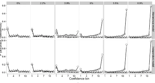
criterion parameter (M = 1364.9). As can be seen from Fig. 9, both the hierarchical logistic 586
model with task criterion fixed at zero and the hierarchical logistic model including a free 587
task criterion parameter provided qualitatively good accounts of the distributions of 588
discrimination accuracy and confidence ratings.
589
4.2.1 Is there support for the independent model?
590
Independent models of metacognition only provided the best model fit in 30% of the 591
participants according to the BIC, and in 40% of the participants according to the AICc. The 592
Bayes factor analysis indicated evidence against the hypothesis that independent models are 593
more likely to attain the best fit both in terms of BIC, BF10 = 0.19, as well as in terms of 594
AICc, BF10 = 0.29. This result implies that prior beliefs that a flavor of the independent 595
models is the generative model of the present data should be attenuated. Accordingly, 596
estimates of metacognition in the present data set based on GLM slopes are likely to be 597
affected by rating criteria.
598
4.2.2 Can the primary task criterion be fixed at 0?
599
Models with the primary task criterion fixed at zero attained the best model fit in 60% of the 600
participants according to the BIC, and in 40% according to the AICc. The Bayes factor 601
analysis does not provide any support in favor of the hypothesis that models with the primary 602
task criterion fixed at zero are associated with better BICs, BF10 = 1.02. However, there was 603
evidence against the hypothesis that models with the primary task criterion fixed at zero are 604
associated with better AICcs, BF10 = 0.29. Consequently, there is some indication that GLM 605
slopes in the present data would also influenced by the primary task criterion, but the 606
evidence is not consistent.
607
4.2.3 Is the evidence distributed logistically?
608
Models based on the assumption of logistic distributions achieved the minimal BIC in 85% of 609
the participants according to BIC and even in 90% according to AICc.. The Bayes factors 610
indicated strong evidence that the logistic models were more likely to produce better fits than 611
Gaussian models, both in terms of BIC, BF10 = 56.1, as well with regard to AICc, BF10 = 612
231.6. This means that only one out of the three conditions for logistic regression slopes to be 613
independent of criteria was met in the present data set.
614
4.2.4 Can the model underlying simulated data be recovered?
615
Fig. 10 shows the results of the model recovery analysis of data simulated according to the 616
independent logistic model with fixed task criterion (squares) and data generated according to 617
the hierarchical Gaussian model with a free task criterion (circles).
618
As can be seen from the panels on the left, when the data was simulated according to the 619
independent logistic model with fixed task criterion, the model was nearly always correctly 620
identified as being one of the independent models. However, when the true model was the 621
hierarchical Gaussian model with free task criterion, the model was relatively often 622
misclassified as independent: When the trial number was small (N ≤ 200), model recovery 623
was even below chance. 5000 trials were required to obtain a tolerable recovery rate of 624
approximately 70%. Increasing the trial number even more did not substantially improve 625
model recovery.
626
The central panels of Fig. 10 show model recovery with respect to the free primary task 627
criterion vs. the primary task criterion fixed at 0. For the BIC as model selection criterion, 628
5000 trials were necessary to detect the free task criterion parameter with a tolerable accuracy 629
of 70%. In contrast, for the AICc, 1200 trials were sufficient to reach 70%. Notably, the AICc 630
does not favor models with smaller number of parameter as heavily as the BIC does. It can 631
also be seen that model recovery accuracy decreased with trial number for the independent 632
logistic model with fixed task criterion (dotted lines). However, at the same time, model 633
recovery accuracy increased with sample size for the hierarchical Gaussian model with free 634
task criterion (straight lines). An explanation for this pattern may be that AICc and BIC both 635
favor more parsimonious models. For small sample sizes, both AICc and BIC prefer models 636
with a smaller number of parameters, which is why models are selected where the primary 637
task criterion is fixed at 0. The bias towards smaller results will result in a correct 638
classification with respect to the primary task criterion when the true model is the 639
independent logistic model with fixed task criterion, but an error will occur when the true 640
model is the hierarchical Gaussian model with free task criterion.
641
Finally, model recovery with respect to logistic and Gaussian distributions is depicted in the 642
right panels of Fig. 10. For large sample sizes, logistic distributions were more often correctly 643
identified than Gaussians. However, 1200 trials were sufficient to obtain a tolerable recovery 644
rate of approximately 70% for both distributions.
645
5 Discussion 646
The analysis presented here investigated whether GLM slopes as measures of metacognition 647
are biased by the spread of rating criteria and the primary task criterion. We showed 648
analytically that logistic regression slopes are independent from rating criteria only according 649
to one specific model of metacognition: the independent model based on logistic 650
distributions. When other distributions were assumed, when other link functions were used, 651
or when a hierarchical model was adopted, regression slopes always depended on the spread 652
of rating criteria. The direction and magnitude of these effects depended on the other model 653
parameters. The primary task criterion was related to regression slopes in all considered 654
models. Depending on the model parameters, the relationship between slopes and task 655
criterion were increasing, decreasing, or even u-shaped. An analysis of regression intercepts 656
revealed that intercepts were insensitive to rating criteria when the amount of metacognition 657
was too low. In addition, we examined if these models can be identified empirically on an 658
existing data set, observing that a massive number of trials is required to distinguish between 659
hierarchical and independent models with tolerable accuracy.
660
5.1 Is logistic regression a biased measure of metacognitive sensitivity?
661
When the aim of a study is to estimate the degree of metacognitive sensitivity, it is generally 662
accepted that a suitable measure should be independent from the primary task criterion and 663
rating criteria (Barrett et al., 2013). However, the present study revealed that logistic 664
regression slopes depend on the primary task criterion independent of the underlying model 665
of metacognition. Logistic regression slopes also depend on rating criteria except for one 666
specific model of metacognition: When the sensory evidence considered for primary task 667
responses is stochastically independent from the sensory evidence used in rating decisions, 668
and when these two types of evidence both form logistic distributions, then logistic regression 669
slopes are independent from rating criteria. This means that when researchers encounter an 670
empirical effect on logistic regression slopes, without knowledge about the underlying model 671
of metacognition, there will be at least three possible explanations for the effect: (i) the effect 672
can be mediated by participants’ degree of metacognition of the processes engaged in 673
performing the task, (ii) the effect might also be due to participants’ bias towards one of the 674
task alternatives, and (iii) the effect may also depend entirely on differences how liberal or 675
conservative participants’ rating criteria are. Likewise, researchers might be unable to 676
observe real effects on participants’ degree of metacognition when there is also a difference 677
between participants’ bias or between rating criteria because the effects of metacognition and 678
criteria could balance out.
679
5.2 Does the present analysis generalize to other models of decision-making and 680
metacognition?
681
The present analysis was based on specific assumptions about the decision process as well as 682
the cognitive model underlying metacognition. Concerning the decision process, we assumed 683
the standard SDT model. Concerning metacognition, only two models, the hierarchical and 684
the independent model were considered. Is it reasonable to assume that the characteristics of 685
GLM slopes outlined here generalize to other models of decision-making and metacognition?
686
As the literature provides a multitude of competing models of decision making, confidence 687
and / or metacognition, it is not feasible to investigate the eligibility of logistic regression for 688
each model proposed in the literature. Examples for different models include the bounded 689
accumulation model (Kiani, Corthell, & Shadlen, 2014), the collapsing confidence boundary 690
model (Moran, Teodorescu, & Usher, 2015), the consensus model (Paz, Insabato, Zylberberg, 691
Deco, & Sigman, 2016), the reaction time account (Ratcliff, 1978), the self-evaluation model 692
(Fleming & Daw, 2016), and two-stage signal detection theory (Pleskac & Busemeyer, 2010).
693
The attempt seems even futile because the number of models in the literature is continuously 694
increasing. However, the two models tested here represent two complementary prototypes of 695
models of metacognition: The hierarchical model is the simplest possible variant of models 696
where the evidence used for the decision between the primary task alternatives also informs 697
the decision between different rating criteria. The view that the evidence used in the decision 698
process is also involved in metacognition is a standard tenet of theories about metacognition.
699
In contrast, the independent model assumes that evidence used for the rating decision is 700
sampled entirely independently from the evidence used for the task response. It is an open 701
question whether datasets exist that can be conveniently described by the independent model.
702
The majority of existing models in the literature are closely related to one of the two models 703
or the models constitute a combination of the two models. For example, post-decisional 704
accumulation models can be seen as a combination of the hierarchical and the independent 705
model, where a second, independent sample of evidence is acquired later in time than the 706
sensory evidence used for performing the task (Moran et al., 2015; Pleskac & Busemeyer, 707
2010). When a model assumes that rating decisions are informed by both evidence considered 708
in the primary task as well as evidence sampled in parallel, it is reasonable to expect that 709
biases apparent in the hierarchical and the independent model persist when the two sources of 710
evidence are combined.
711
Of course, it is still possible that there will be new theories which imply that logistic 712
regression is not affected by primary task criteria and rating criteria. However, the 713
implications of the present study do not require that such a model does not exist. What the 714
study implies is that according to plausible models of metacognition, logistic regression is 715
affected from primary task criterion and rating criteria. As a consequence, researchers who 716
wish to use logistic regression to measure metacognitive sensitivity need to show that their 717
effects cannot be alternatively explained by rating criteria and primary task criteria.
718
5.3 Can the independent model be empirically identified?
719
To exclude the possibility that effects on regression slopes are not caused or masked by rating 720
criteria, it would be useful to identify the underlying model of metacognition. Unfortunately, 721
the present model recovery analysis revealed that the amount of trials required to correctly 722
classify a true underlying hierarchical Gaussian model is massive. Moreover, the hierarchical 723
Gaussian model was still occasionally misclassified as independent or logistic even with 724
extreme trial numbers. In a similar comparison between different models of metacognition, 725
two thirds of the participants were excluded to reduce noise in the data and improve model 726
selection, implying that these models are also not trivial to distinguish based on other data 727
sets (Maniscalco & Lau, 2016). Likewise, Gaussian and logistic distributions are known to 728
produce similar results in many applications (DeCarlo, 1998; Wickens, 2002). Consequently, 729
when researchers intend to model the cognitive architecture of metacognition, they will need 730
to ensure that both the sample size and the trial number are sufficiently large to ensure that 731
classification errors are outnumbered by correct classifications. However, for those 732
researchers who are only interested in measuring metacognition, the standard application of 733
logistic regression as measure of metacognitive sensitivity, cognitive modeling will usually 734
not be a feasible option because the number of trials in standard experiments is typically too 735
small. Future studies might be able to provide more efficient methods to distinguish between 736
the hierarchical Gaussian and the independent logistic model.
737